
Machine Learning Predictive Analysis of Liquefaction Resistance for Sandy Soils Enhanced by Chemical Injection


Abstract
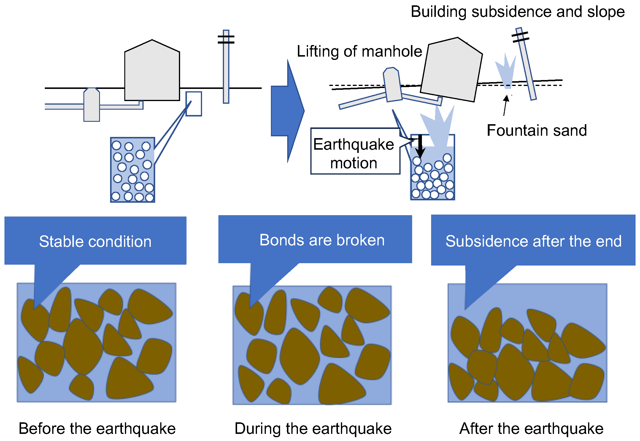
:1. Introduction
2. General Evaluation and Countermeasures to Liquefaction of Sandy Soils
2.1. Chemical Injection Method
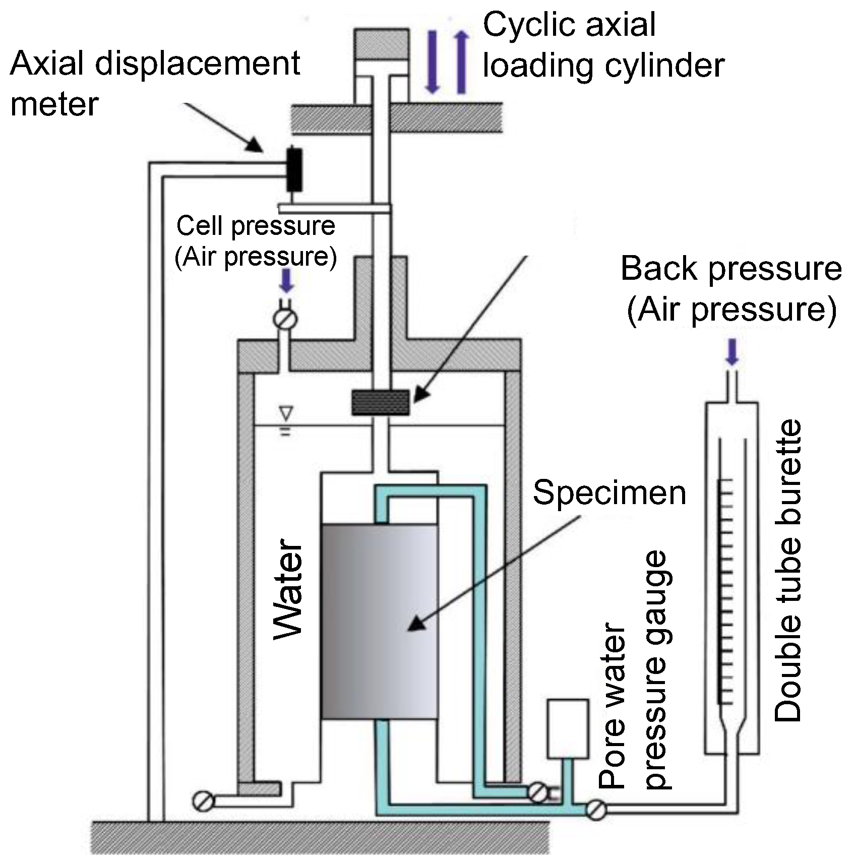
2.2. Cyclic Undrained Triaxial Test
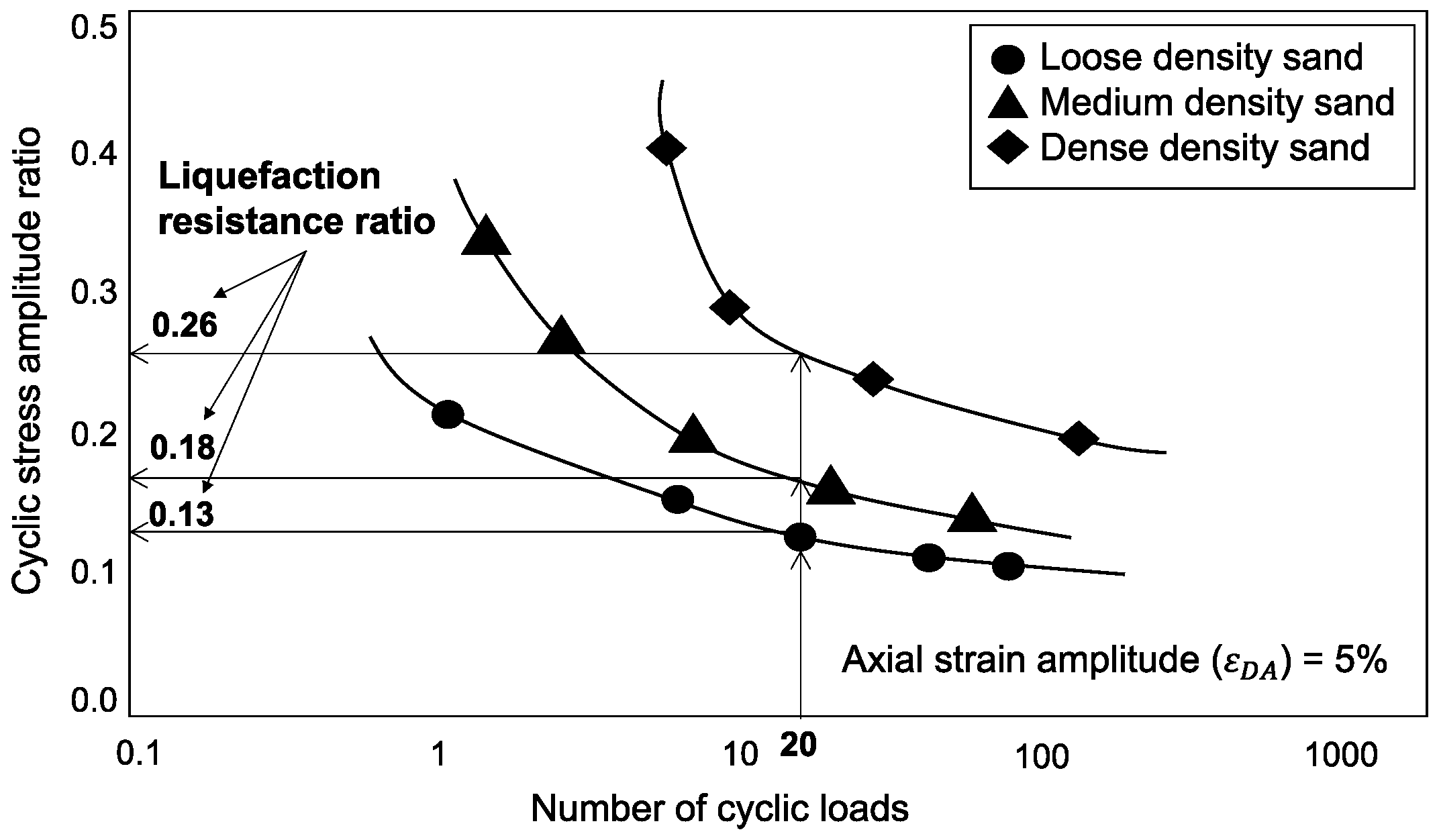
2.3. Liquefaction Resistance Ratio
3. Machine Learning Predictive Analysis
3.1. Ensemble Learning
- (1)
- Interpretability and transparency: Decision trees provide a clear and interpretable structure, making it easy to understand how predictions are made. This is particularly important in this study because it involves complex geotechnical data, where providing clear insight into how the model reaches its conclusions is critical to gaining acceptance and trust from the engineering community.
- (2)
- Handling of non-linear relationships: The nature of the dataset in this study, which includes various soil parameters and their interactions, exhibits non-linear patterns. Gradient boosting decision trees are adept at handling such non-linear relationships, making them a suitable choice for predictive analysis in this study.
- (3)
- Flexibility with different types of data: The dataset in this study includes a mix of numeric and categorical variables (such as soil type, chemical composition, etc.). Decision trees can handle this variety without extensive preprocessing, simplifying the modeling process.
- (4)
- Robustness against outliers and missing values: Decision trees are less sensitive to outliers and can handle missing data efficiently, which is a significant advantage given the variability and occasional gaps in geotechnical data.
- (5)
- Effective with ensemble methods: Ensemble learning techniques, which combine multiple machine learning models to improve prediction accuracy, were used. Decision trees integrate well with such ensemble methods (e.g., gradient boosting decision tree) and often result in models that are more accurate and robust than those based on a single algorithm.
3.2. Preparation of Dataset
3.2.1. Details of Training Data
3.2.2. Details of Test Data
3.3. Distinguishing Explanatory and Target Variables
3.4. Evaluation of Prediction Accuracy
- (1)
- Interpretability in the context of geotechnical engineering: In geotechnical engineering, particularly in studies involving practitioners and engineers, the interpretability of the model output is critical. , as a widely recognized and understood metric, provides a clear and direct measure of how well the model’s predictions match the actual observed data.
- (2)
- Quantifying the explanation of variance: The primary goal of this study was to develop a model that could accurately predict liquefaction resistance based on various input characteristics. effectively quantifies the proportion of variance in the dependent variable that can be predicted from the independent variables, which directly aligns with the goal of this study.
- (3)
- Model evaluation in machine learning: In the context of machine learning, particularly ensemble methods, is still a relevant metric for evaluating predictive models. It provides a concise summary of model performance, especially when dealing with continuous outcome variables, as in this study.
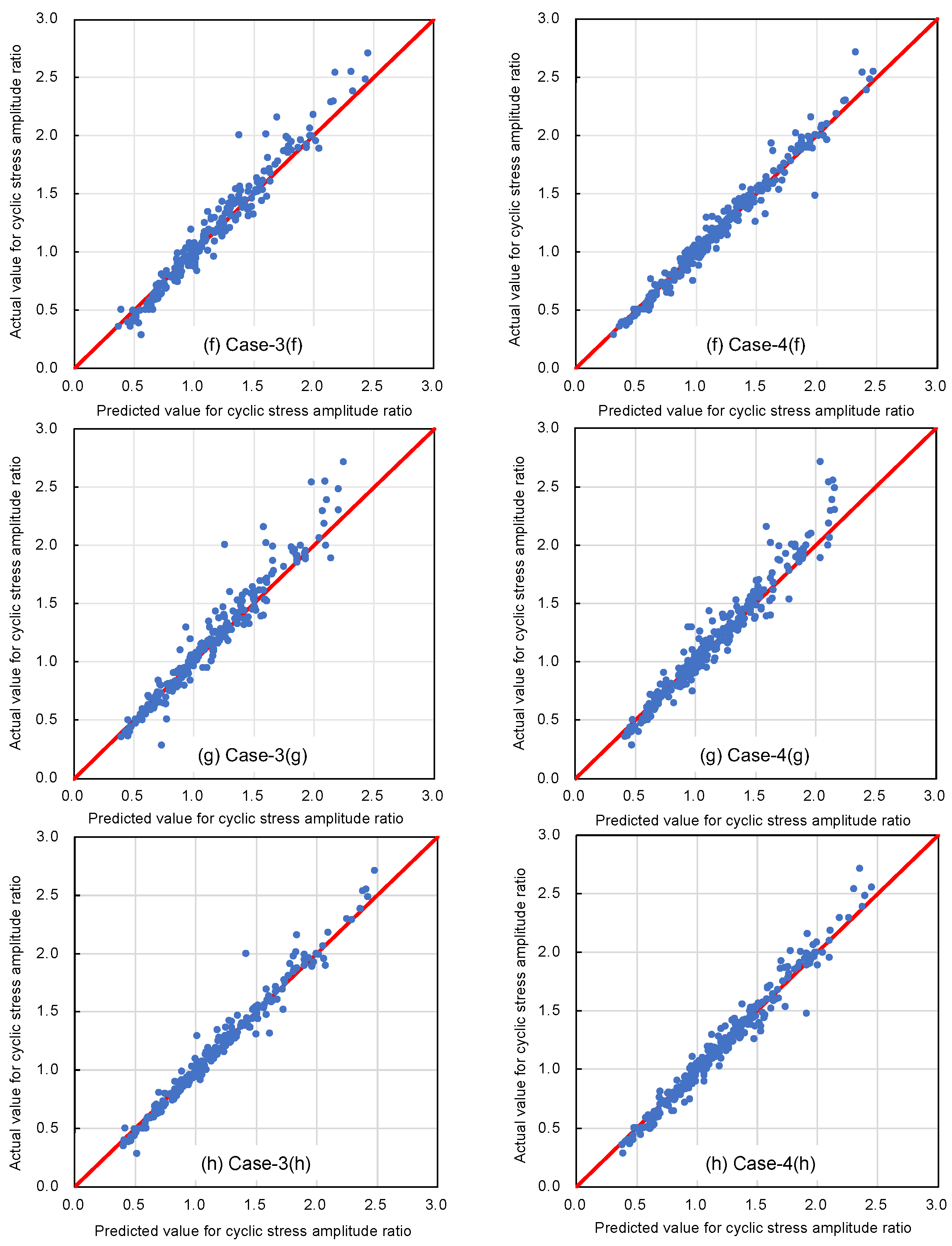
4. Results and Discussion
4.1. Selecting Target Variables
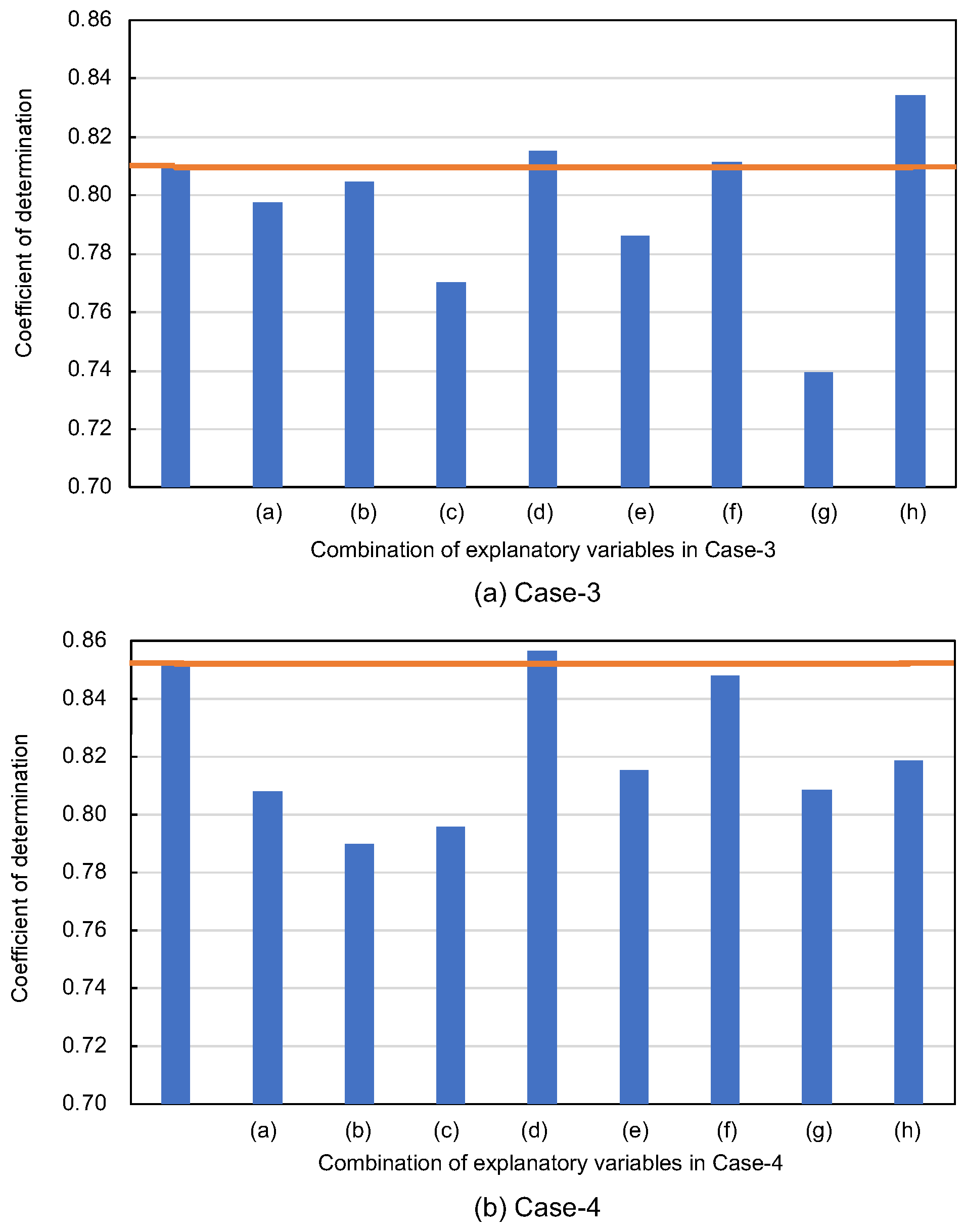
4.2. Selecting Explanatory Variables
5. Conclusions
- (1)
- For the development of a predictive model, it is highly recommended to designate the liquefaction resistance ratio as a dependent variable and the other parameters as explanatory variables. This approach allows for a more focused analysis and provides more reliable predictions of the soil behavior under liquefaction conditions.
- (2)
- The exploration of combinations of explanatory variables revealed that using all available variables tends to produce a more stable coefficient of determination (). This stability is critical to the reliability of the model, especially in applications where precision is paramount.
- (3)
- Including the liquefaction resistance ratio in the training dataset significantly increases the predictive accuracy of the model. This finding underscores the importance of this particular variable in understanding and predicting the behavior of chemically enhanced sandy soils under stress.
- (4)
- The results of using AI for making predictions highlight the potential of accurately predicting liquefaction resistance using historical data. This approach not only saves time and resources, but also opens new avenues for studies in soil mechanics and geotechnical engineering.
- (5)
- In addition, this study aimed to validate the effectiveness of the solution-type chemical improvement of sandy soils against liquefaction through an AI-based analysis of existing data from cyclic undrained triaxial tests. The results of this study confirmed that high-precision predictions are achievable using the explanatory variables listed in Table 1. In particular, excluding uniaxial compressive strength as an explanatory variable resulted in the highest accuracy, followed closely by scenarios using all explanatory variables. This suggests a nuanced relationship between the variables and their predictive power that warrants further investigation.
Author Contributions
Funding
Data Availability Statement
Conflicts of Interest
References
- Kuribayashi, E.; Tatsuoka, F. Brief review of liquefaction during earthquakes in Japan. Soils Found. 1975, 15, 81–92. [Google Scholar] [CrossRef] [PubMed]
- Huang, Y.; Yu, M. Review of soil liquefaction characteristics during major earthquakes of the twenty-first century. Nat. Hazards 2013, 65, 2375–2384. [Google Scholar] [CrossRef]
- Hasheminezhad, A.; Bahadori, H. Three dimensional finite difference simulation of liquefaction phenomenon. Int. J. Geotech. Eng. 2019, 15, 245–251. [Google Scholar] [CrossRef]
- Nakao, K.; Inazumi, S.; Takahashi, T.; Nontananandh, S. Numerical simulation of the liquefaction phenomenon by MPSM-DEM coupled CAES. Sustainability 2022, 14, 7517. [Google Scholar] [CrossRef]
- Lo, R.C.; Wang, Y. Lessons learned from recent earthquakes-geoscience and geotechnical perspectives. In Advances in Geotechnical Earthquake Engineering—Soil Liquefaction and Seismic Safety of Dams and Monuments; IntechOpen: Rijeka, Croatia, 2012; pp. 1–42. [Google Scholar] [CrossRef]
- Hazout, L.; Zitouni, Z.E.A.; Belkhatir, M.; Schanz, T. Evaluation of static liquefaction characteristics of saturated loose sand through the mean grain size and extreme grain sizes. Geotech. Geol. Eng. 2017, 35, 2079–2105. [Google Scholar] [CrossRef]
- Bao, X.; Ye, B.; Ye, G.; Zhang, F. Co-seismic and post-seismic behavior of a wall type breakwater on a natural ground composed of liquefiable layer. Nat. Hazards 2016, 83, 1799–1819. [Google Scholar] [CrossRef]
- Bao, X.; Jin, Z.; Cui, H.; Chen, X.; Xie, X. Soil liquefaction mitigation in geotechnical engineering: An overview of recently developed methods. Soil Dyn. Earthq. Eng. 2019, 120, 273–291. [Google Scholar] [CrossRef]
- Gallagher, P.M.; Pamuk, A.; Abdoun, T. Stabilization of liquefiable soils using colloidal silica grout. J. Mater. Civ. Eng. 2007, 19, 33–40. [Google Scholar] [CrossRef]
- Sayehvand, S.; Kalantari, B. Use of grouting method to improve soil stability against liquefaction—A review. Electron. J. Geotech. Eng. 2012, 17, 1559–1566. [Google Scholar]
- Verma, H.; Ray, A.; Rai, R.; Gupta, T.; Mehta, N. Ground improvement using chemical methods: A review. Heliyon 2021, 7, e07678. [Google Scholar] [CrossRef]
- Yoon, J.C.; Su, S.W.; Kim, J.M. Method for prevention of liquefaction caused by earthquakes using grouting applicable to existing structures. Appl. Sci. 2023, 13, 1871. [Google Scholar] [CrossRef]
- Motohashi, T.; Sasahara, S.; Inazumi, S. Strength assessment of water-glass sand mixtures. Gels 2023, 9, 850. [Google Scholar] [CrossRef]
- Yoshimi, Y.; Tanaka, K.; Tokimatsu, K. Liquefaction resistance of a partially saturated sand. Soils Found. 1989, 29, 157–162. [Google Scholar] [CrossRef] [PubMed]
- Mele, L.; Flora, A. On the prediction of liquefaction resistance of unsaturated sands. Soil Dyn. Earthq. Eng. 2019, 125, 105689. [Google Scholar] [CrossRef]
- Park, S.S.; Nong, Z.Z.; Woo, S.W. Liquefaction resistance of Pohang sand. In Earthquake Geotechnical Engineering for Protection and Development of Environment and Constructions; CRC Press: London, UK, 2019; pp. 4359–4365. [Google Scholar]
- Khashila, M.; Hussien, M.N.; Karray, M.; Chekired, M. Liquefaction resistance from cyclic simple and triaxial shearing: A comparative study. Acta Geotech. 2021, 16, 1735–1753. [Google Scholar] [CrossRef]
- Ni, X.Q.; Zhang, Z.; Ye, B.; Zhang, S. Unique relation between pore water pressure generated at the first loading cycle and liquefaction resistance. Eng. Geol. 2022, 296, 106476. [Google Scholar] [CrossRef]
- Toyota, H.; Takada, S. Variation of liquefaction strength induced by monotonic and cyclic loading histories. J. Geotech. Geoenviron. Eng. 2017, 143, 04016120. [Google Scholar] [CrossRef]
- Zhang, J.; Yang, Z.; Yang, Q.; Yang, G.; Li, G.; Liu, J. Liquefaction behavior of fiber-reinforced sand based on cyclic triaxial tests. Geosynth. Int. 2021, 28, 316–326. [Google Scholar] [CrossRef]
- Amer, M.I.; Kovacs, W.D.; Aggour, M.S. Cyclic simple shear size effects. J. Geotech. Eng. 1987, 113, 7, 693–707. [Google Scholar] [CrossRef]
- Nong, Z.Z.; Park, S.S.; Lee, D.E. Comparison of sand liquefaction in cyclic triaxial and simple shear tests. Soils Found. 2021, 61, 1071–1085. [Google Scholar] [CrossRef]
- Nong, Z.Z.; Park, S.S.; Jeong, S.W.; Lee, D.E. Effect of cyclic loading frequency on liquefaction prediction of sand. Appl. Sci. 2021, 10, 4502. [Google Scholar] [CrossRef]
- Arpit, J.; Mittal, S.; Shukla, S.K. Liquefaction proneness of stratified sand-silt layers based on cyclic triaxial tests. J. Rock Mech. Geotech. Eng. 2023, 15, 1826–1845. [Google Scholar] [CrossRef]
- Hyodo, M.; Yasuhara, K.; Hirao, K. Prediction of clay behaviour in undrained and partially drained cyclic triaxial tests. Soils Found. 1992, 32, 117–127. [Google Scholar] [CrossRef]
- Gu, C.; Wang, J.; Cai, Y.; Yang, Z.; Gao, Y. Undrained cyclic triaxial behavior of saturated clays under variable confining pressure. Soil Dyn. Earthq. Eng. 2012, 40, 118–128. [Google Scholar] [CrossRef]
- Ghayoomi, M.; Suprunenko, G.; Mirshekari, M. Cyclic triaxial test to measure strain-dependent shear modulus of unsaturated sand. Int. J. Geomech. 2017, 17, 04017043. [Google Scholar] [CrossRef]
- Dong, X.; Yu, Z.; Cao, W.; Shi, Y.; Ma, Q. A survey on ensemble learning. Front. Comput. Sci. 2020, 14, 241–258. [Google Scholar] [CrossRef]
- Chongzhi, W.; Lin, W.; Zhang, W. Assessment of undrained shear strength using ensemble learning based on Bayesian hyperparameter optimization. In Modeling in Geotechnical Engineering; Academic Press: Cambridge, MA, USA, 2021; pp. 309–326. [Google Scholar] [CrossRef]
- Wang, Z.Z.; Hu, Y.; Guo, X.; He, X.; Kek, H.Y.; Ku, T.; Goh, S.H.; Leung, C.F. Predicting geological interfaces using stacking ensemble learning with multi-scale features. Can. Geotech. J. 2023, 60, 7. [Google Scholar] [CrossRef]
- Shahin, M.A. Artificial intelligence in geotechnical engineering: Applications, modeling aspects, and future directions. In Metaheuristics in Water, Geotechnical and Transport Engineering; Elsevier: Amsterdam, The Netherlands, 2013; pp. 169–204. [Google Scholar]
- Jong, S.C.; Ong, D.E.L.; Oh, E. State-of-the-art review of geotechnical-driven artificial intelligence techniques in underground soil-structure interaction. Tunn. Undergr. Space Technol. 2021, 113, 103946. [Google Scholar] [CrossRef]
- Baghbani, A.; Choudhury, T.; Costa, S.; Reiner, J. Application of artificial intelligence in geotechnical engineering: A state-of-the-art review. Earth-Sci. Rev. 2022, 228, 103991. [Google Scholar] [CrossRef]
- Sharma, S.; Ahmed, S.; Naseem, M.; Alnumay, W.S.; Singh, S.; Cho, G.H. A survey on applications of artificial intelligence for pre-parametric project cost and soil shear-strength estimation in construction and geotechnical engineering. Sensors 2021, 21, 463. [Google Scholar] [CrossRef]
- Huang, Y.; Wen, Z. Recent developments of soil improvement methods for seismic liquefaction mitigation. Nat. Hazards 2015, 76, 1927–1938. [Google Scholar] [CrossRef]
- Cardellicchio, A.; Ruggieri, S.; Nettis, A.; Renò, V.; Uva, G. Physical interpretation of machine learning-based recognition of defects for the risk management of existing bridge heritage. Eng. Fail. Anal. 2023, 149, 107237. [Google Scholar] [CrossRef]
- Mele, L.; Tian, J.T.; Lirer, S.; Flora, A.; Koseki, J. Liquefaction resistance of unsaturated sands: Experimental evidence and theoretical interpretation. Géotechnique 2019, 69, 541–553. [Google Scholar] [CrossRef]
- Fahim, A.K.F.; Rahman, M.Z.; Hossain, M.S.; Kamal, A.M. Liquefaction resistance evaluation of soils using artificial neural network for Dhaka City, Bangladesh. Nat. Hazards 2022, 113, 933–963. [Google Scholar] [CrossRef]
- Kotsiantis, S.B.; Zaharakis, I.D.; Pintelas, P.E. Machine learning: A review of classification and combining techniques. Artif. Intell. Rev. 2006, 26, 159–190. [Google Scholar] [CrossRef]
- Pólvora, A.; Nascimento, S.; Lourenço, J.S.; Scapolo, F. Blockchain for industrial transformations: A forward-looking approach with multi-stakeholder engagement for policy advice. Technol. Forecast. Soc. Change 2020, 157, 120091. [Google Scholar] [CrossRef]
- Tuttle, M.P.; Hartleb, R.; Wolf, L.; Mayne, P.W. Paleoliquefaction studies and the evaluation of seismic hazard. Geosciences 2019, 9, 311. [Google Scholar] [CrossRef]
- Dhakal, R.; Cubrinovski, M.; Bray, J.D. Geotechnical characterization and liquefaction evaluation of gravelly reclamations and hydraulic fills (Port of Wellington, New Zealand). Soils Found. 2020, 60, 1507–1531. [Google Scholar] [CrossRef]
- Yang, M.; Taiebat, M.; Radjaï, F. Liquefaction of granular materials in constant-volume cyclic shearing: Transition between solid-like and fluid-like states. Comput. Geotech. 2022, 148, 104800. [Google Scholar] [CrossRef]
- Mitchell, J.K. Mitigation of liquefaction potential of silty sands. In Research to Practice in Geotechnical Engineering; American Society of Civil Engineers: Reston, VA, USA, 2008; pp. 433–451. [Google Scholar] [CrossRef]
- Kramer, S.L.; Mitchell, R.A. Ground motion intensity measures for liquefaction hazard evaluation. Earthq. Spectra 2006, 22, 413–438. [Google Scholar] [CrossRef]
- Zhou, Z.H. Ensemble Methods: Foundations and Algorithms; Chapman & Hall/CRC Machine Learning & Pattern Recognition; CRC Press: Boca Raton, FL, USA, 2012. [Google Scholar]
- Gurney, K. An Introduction to Neural Networks, 1st ed.; CRC Press: Boca Raton, FL, USA, 1997. [Google Scholar]
- Zhao, Z.; Chow, T.L.; Rees, H.W.; Yang, Q.; Xing, Z.; Meng, F.R. Predict soil texture distributions using an artificial neural network model. Comput. Electron. Agric. 2009, 65, 36–48. [Google Scholar] [CrossRef]
- Zhong, L.; Guo, X.; Xu, Z.; Ding, M. Soil properties: Their prediction and feature extraction from the LUCAS spectral library using deep convolutional neural networks. Geoderma 2021, 402, 115366. [Google Scholar] [CrossRef]
- Pham, B.T.; Nguyen, M.D.; Ly, H.B.; Pham, T.A.; Hoang, V.; Le, V.H.; Le, T.T.; Nguyen, H.Q.; Bui, G.L. Development of artificial neural networks for prediction of compression coefficient of soft soil. In Proceedings of the 5th International Conference on Geotechnics, Civil Engineering Works and Structures, Virtual, 18–20 October 2020; pp. 1167–1172. [Google Scholar]
- Chakraborty, D.; Elhegazy, H.; Elzarka, H.; Gutierrez, L. A novel construction cost prediction model using hybrid natural and light gradient boosting. Adv. Eng. Inform. 2020, 46, 101201. [Google Scholar] [CrossRef]
- Lee, S.; Vo, T.P.; Thai, H.T.; Lee, J.; Patel, V. Strength prediction of concrete-filled steel tubular columns using Categorical Gradient Boosting algorithm. Eng. Struct. 2021, 238, 112109. [Google Scholar] [CrossRef]
- Guo, R.; Fu, D.; Sollazzo, G. An ensemble learning model for asphalt pavement performance prediction based on gradient boosting decision tree. Int. J. Pavement Eng. 2022, 23, 3633–3646. [Google Scholar] [CrossRef]
- Nakagawa, S.; Johnson, P.C.D.; Schielzeth, H. The coefficient of determination R2 and intra-class correlation coefficient from generalized linear mixed-effects models revisited and expanded. J. R. Soc. Interface 2017, 14, 1–11. [Google Scholar] [CrossRef]


| Category | Variable Elements |
|---|---|
| Condition parameters for specimens of chemically improved sandy soils | Dry density (g/cm3) |
| Fine particle content (%) | |
| Effective confining pressure (kN/m2) | |
| Unconfined compressive strength (kN/m2) | |
| Silica gel concentration of injected chemical solution (%) | |
| Increase in silica content (mg/g) | |
| Results obtained by cyclic undrained triaxial test | Number of cycles to reach 5% strain in both amplitudes |
| Number of cycles to reach 95% excess pore pressure ratio | |
| Cyclic stress amplitude ratio | |
| Liquefaction resistance ratio * |
| Case | Explanatory Variables | Target Variables |
|---|---|---|
| Case-1 | Variable elements shown in Table 1 excluding the liquefaction resistance ratio and the target variable | Number of cycles to reach 5% strain in both amplitudes |
| Case-2 | Variable elements shown in Table 1 excluding the liquefaction resistance ratio and the target variable | Number of cycles to reach 95% excess pore pressure ratio |
| Case-3 | Variable elements shown in Table 1 excluding the liquefaction resistance ratio and the target variable | Cyclic stress amplitude ratio |
| Case-4 | Variable elements shown in Table 1 excluding the target variable | Cyclic stress amplitude ratio |
| Variable | Variable Elements | Data for 2 of 272 Specimens | |
|---|---|---|---|
| Explanatory variables | Dry density (g/cm3) | 1.684 | 1.484 |
| Effective confining pressure (kN/m2) | 90 | 165 | |
| Fine particle content (%) | 14.8 | 11.4 | |
| Unconfined compressive strength (kN/m2) | 539 | 483 | |
| Silica gel concentration of injected chemical solution (%) | 12 | 12 | |
| Increase in silica content (mg/g) | 11.62 | 7.79 | |
| Number of cycles to reach 5% strain in both amplitudes | 18 | 6.5 | |
| Number of cycles to reach 95% excess pore pressure ratio | 37 | 38.4 | |
| Target variable | Repetitive stress amplitude ratio | ||
| Case-3 and Case-4 | ||||||||
|---|---|---|---|---|---|---|---|---|
| Explanatory Variables | (a) | (b) | (c) | (d) | (e) | (f) | (g) | (h) |
| Dry density (g/cm3) | x | |||||||
| Effective confining pressure (kN/m2) | x | |||||||
| Fine particle content (%) | x | |||||||
| Unconfined compressive strength (kN/m2) | x | |||||||
| Silica gel concentration of injected chemical solution (%) | x | |||||||
| Increase in silica content (mg/g) | x | |||||||
| Number of cycles to reach 5% strain in both amplitudes | x | |||||||
| Number of cycles to reach 95% excess pore pressure ratio | x | |||||||
Disclaimer/Publisher’s Note: The statements, opinions and data contained in all publications are solely those of the individual author(s) and contributor(s) and not of MDPI and/or the editor(s). MDPI and/or the editor(s) disclaim responsibility for any injury to people or property resulting from any ideas, methods, instructions or products referred to in the content. |
© 2024 by the authors. Licensee MDPI, Basel, Switzerland. This article is an open access article distributed under the terms and conditions of the Creative Commons Attribution (CC BY) license (https://creativecommons.org/licenses/by/4.0/).
Share and Cite
Cong, Y.; Motohashi, T.; Nakao, K.; Inazumi, S. Machine Learning Predictive Analysis of Liquefaction Resistance for Sandy Soils Enhanced by Chemical Injection. Mach. Learn. Knowl. Extr. 2024, 6, 402-419. https://doi.org/10.3390/make6010020
Cong Y, Motohashi T, Nakao K, Inazumi S. Machine Learning Predictive Analysis of Liquefaction Resistance for Sandy Soils Enhanced by Chemical Injection. Machine Learning and Knowledge Extraction. 2024; 6(1):402-419. https://doi.org/10.3390/make6010020
Chicago/Turabian StyleCong, Yuxin, Toshiyuki Motohashi, Koki Nakao, and Shinya Inazumi. 2024. "Machine Learning Predictive Analysis of Liquefaction Resistance for Sandy Soils Enhanced by Chemical Injection" Machine Learning and Knowledge Extraction 6, no. 1: 402-419. https://doi.org/10.3390/make6010020