1. Introduction
Medical imaging plays a pivotal role in many medical diagnostic tasks. In order to obtain an accurate diagnosis, high-quality image acquisition and interpretation are both required [
1]. Acquisition technology has significantly improved in recent decades, with scanners that enable higher resolution and shortened acquisition times having become available [
2,
3,
4,
5]. Furthermore, the image interpretation process has undergone major advancements over the last decade due to the development of deep learning methods and access to high-performance computational resources. Deep learning has been shown to yield State-of-the-Art performance in terms of accuracy and computational speed [
6,
7,
8,
9,
10]. The combination of these technological advancements, thus, has the potential to revolutionize medical imaging, playing a key role as a supporting tool in the radiological workflow [
11]. The U.S. Food and Drug Administration (FDA) has approved a few diagnostic procedures utilizing deep learning and artificial intelligence (AI) technologies [
12,
13,
14]. Nonetheless, three major challenges remain for deep diagnostic models, namely, (1) a lack of access to interpreted medical images and data, which are required for the training process; (2) limited reliability and robustness to noise or other unknown perturbations in the data acquisition process [
15,
16,
17]; and (3) limited ability to generalize to data sets characterized by distributions that differ from that of the training data [
18,
19]. These challenges create the gap that currently exists between theory and practice in terms of incorporating such technology into actual clinical settings.
The performance of a machine learning (ML) algorithm for a given task is typically assessed using metrics such as accuracy, specificity, and sensitivity. However, especially when considering the clinical applicability of such algorithms, robustness is an additional important aspect of performance that should be considered. “Robustness” is a general term that may be referred to in different contexts, such as robustness to deterministic input variations (e.g., contrast) [
17], out-of-distribution (OOD) inputs [
18], random input perturbations or noise [
20], adversarial attacks [
15,
21,
22,
23,
24], and more. The underlying approach at the core of robustness assessment, which is common to these different contexts, is to examine the extent of the variation that may be applied to the algorithm’s input whilst obtaining valid predictions at the output. In any case, evaluating the robustness of a deep learning model intended for clinical tasks should be addressed in addition to its accuracy and specificity metrics, according to the application at hand.
One straightforward approach to increase the robustness of a deep neural network (DNN) to unknown perturbations is data augmentation, where the network is trained on an artificially expanded data set created by applying a modifying transform or adding noise to the existing data [
25]. However, this approach is basically focused on the desired output of the network according to the required task; it does not introduce any new information that may affect the learning process of the network to resemble a human perspective derived from the specific problem or task at hand [
25]. An approach to address this issue that has been discussed in recent years is the inclusion of physics-prior information, which is related to the forward imaging models, into the learning process and/or network design [
26,
27,
28,
29]. The assumption behind the inclusion of physics-prior information is that it may shift the learning mechanism in order to improve the stability of the network [
26]. In addition, it has been shown that the inclusion of such priors may improve the generalization capacity of the network. Furthermore, it has the important advantage of supporting training on smaller data sets or in cases where the clinical ground truth (GT) is unavailable [
26]. The more general concept of the incorporation of domain knowledge into deep learning for medical imaging analysis is thoroughly discussed in [
25].
An additional important issue is the choice of network architecture, which may significantly affect the performance of the network. In [
28], the problem of a neural architecture search in the context of physics-based learning has been addressed, and a scheme for automatically finding an optimal architecture was proposed through a general formulation that is not limited to the medical case. However, the performance of this approach in medical applications has yet to be validated.
A comprehensive survey of works in which the medical knowledge domain is integrated into deep learning techniques has been given in [
25], categorizing the studies according to their medical tasks, namely, disease diagnosis, lesion/organ abnormality detection, and lesion/organ segmentation. An additional central review paper is [
29], which includes an overview of deep learning methods incorporating physics priors for MRI reconstruction tasks. In [
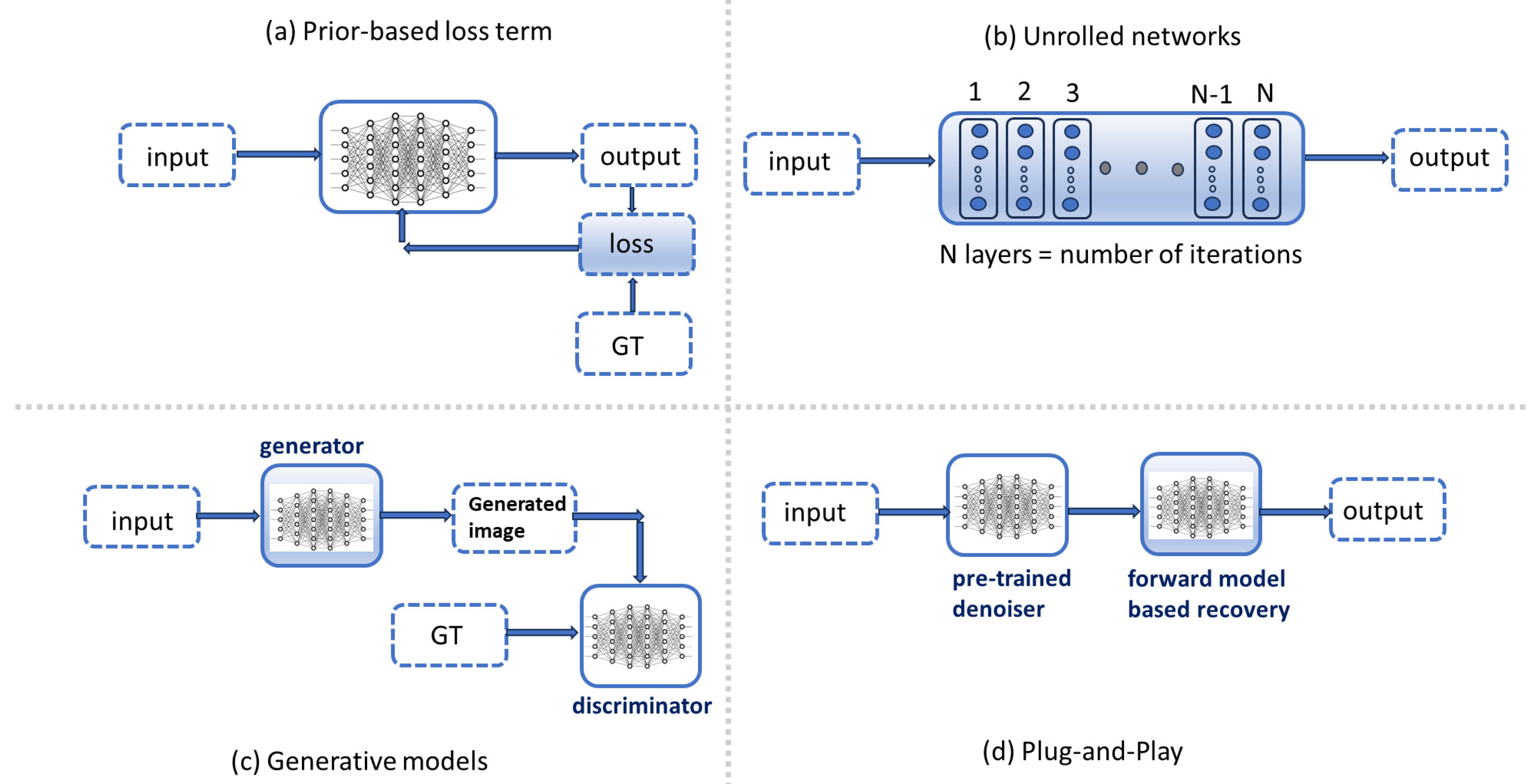
29], physics-based approaches were classified according to the principal mechanisms of inclusion of the physics prior, namely, physics-based loss functions, plug-and-play (PnP) methods, generative models, and unrolled networks.
In this paper, we survey recent studies that have utilized approaches involving the inclusion of prior knowledge into the learning process for various medical imaging modalities, tasks, and applications and discuss how this improves the training mechanism and performance of the deep neural models. We follow the classification method proposed in [
29] and discuss the common thread of the physics-prior-based mechanisms for various imaging modalities, such as diffusion-weighted MRI, ultrasound imaging, and PET-CT, among others. Following this survey, we further propose to extend the approach of physics-based learning to consist of an
explicit physics prior, which describes the relation between the input and output of the forward imaging model, such that the prior is specifically fed into the architecture. Motivated by the applications discussed in the survey, we also introduce a problem formulation for the proposed approach, considering the task of optimal parameter estimation for a highly nonlinear forward physical model. Furthermore, we briefly describe a possible simulated-experiment-based methodology to quantitatively assess the performance of the proposed approach in terms of its generalization ability. To conclude the paper, we outline current challenges and future research directions within this context.
It is important to note that our goal in this paper is by no means to cover all the research papers within the scope of physics-based deep learning; we mainly focus on recent studies, the majority of which are from the previous five or six years and discuss their general common principles within the context of the various physics-prior-based methods. We incorporate references from searched databases including the following publications: Medical Image Analysis, Magnetic Resonance in Medicine, Proceedings of the International Conference on Medical Image Computing and Computer-Assisted Intervention (MICCAI), IEEE Transactions on Medical Imaging, IEEE Signal Processing Magazine, and other IEEE-related databases. We also included additional cross-referenced works not listed in the above search process.
2. Physics-Based Loss Terms
The inclusion of a physics prior as part of the loss term directly affects the learning mechanism of a network, as this means that it is used in the optimization process during training. A straightforward way to include the physics prior as part of the loss term is to simply insert the expression for the physical forward model that relates to the input and output of the network into the loss calculation. (A general scheme is shown in
Figure 1a.) For example, in [
30], an unsupervised physics-based DNN was proposed for the problem of intravoxel incoherent motion (IVIM) model parameter estimation for diffusion-weighted MRI in pancreatic imaging, where the forward model equation was incorporated into the loss function of the network. This enabled iterative learning of the IVIM parameters, which were the required output of the network. The training process was applied for synthetically generated data produced according to the forward model equations, which enabled unsupervised learning without requiring either clinical data or their corresponding ground truth (GT) parameter maps. A similar approach was applied in [
26] for an ophthalmology application, in which the bio-optical parameters of the intraocular lens were required to be accurately evaluated for cataract surgeries. For this purpose, a DNN incorporating the optical ray propagation model in the eye was trained on synthetically generated biometric data. The physics-based loss term included the explicit expressions for the eye’s optical system, and its minimization yielded the required parameters. The proposed training result was shown to be superior to that of systems with a standard training approach, as well as State-of-the-Art intraocular calculation on biometric datasets. Thus, it was concluded that the inclusion of a physics prior into the network’s loss term enabled the generalization of the network model to a wide range of eye biometric data without requiring large clinical data sets.
For problems where explicit forward model expressions are not fully known, a different approach is to express the loss term as an optimization problem whose solution coincides with the model equations. In this manner, the model equations are implicitly integrated into the loss term. For example, in [
31], the problem of producing in silico, patient-specific cardiac mechanical models was discussed. This problem, which may be solved by computationally intensive finite element models (FEMs), was addressed through the use of a deep neural network approach that aims to replace the FEM solution. A cost term that included the effect of the heart microstructure and its contraction was applied in order to avoid the need for heavy and time-consuming finite element model computations. The minimization of this cost function coincided with the solution to the momentum balance equations, which model the dynamics of the heart microstructure. The inclusion of physics priors as part of the loss function, thus, enabled the researchers to bypass heavy computations whilst providing a network with generalization capacity for individualized in silico models.
A different approach to the inclusion of physics priors as part of the loss term has been suggested in [
32], in which a novel method for strain reconstruction maps in ultrasound elastography imaging was proposed. In this study, implicit physics information that relates to the RF data, the tissue displacement, and the predicted elastography map was incorporated into the cost function of the network. The inclusion of the implicit tissue displacement prior (termed “privileged information”) was enabled by applying a strategy to generate triplets of training data, privileged information, and training labels based on numerical biomechanics and ultrasound physics simulations. This physics-based loss term was applied as feedback information to an intermediate layer of the network architecture, whose output was the predicted tissue strain map. This network was demonstrated to outperform previous State-of-the-Art methods on simulated, phantom, and clinical liver and breast imaging data. It was observed that the inclusion of the privileged information in the loss term enabled the researchers to correct the intermediate state of the learning process and narrow the search region of the network parameters, thereby inducing the learning process to converge toward the actual target map.
Another class of physics-based loss term techniques is related to the task of image reconstruction from undersampled data [
29]. Specifically, for undersampled MRI reconstruction, namely, compressed sensing (CS), fast signal acquisition is enabled by subsampling in the k-space (the transform domain). The goal of the network is to find an optimal reconstruction function, which maps the subsampled k-space data into an image close to the MR image that corresponds to the fully sampled data [
29]. Several works have shown that applying a loss term that enforces consistency in the k-space domain may yield improved quality for higher sampling rates, such as in brain MRI [
33,
34]. This may be intuitively explained by interpreting the k-space as frequency domain data. In [
35], a few low-frequency terms from the k-space were included in addition to the consistency enforcement, such that the overall image–domain structure of the MRI image was preserved, and anomaly location uncertainty was avoided. Similarly, in [
18], a transform-based consistency was applied to generate standard-dose PET images from their low-dose counterparts and corresponding multicontrast MRI images. For this purpose, the sinogram-based physics of the PET imaging system was incorporated into the loss function, such that the per-voxel residual in the transform domain was penalized in a similar manner as applied in undersampled MRI reconstruction. The experimental results on brain scans demonstrate that the inclusion of the transform domain loss improved the robustness of the network to out-of-distribution (OOD) data in the form of lower counts [
18].
To conclude this subsection, the inclusion of physics priors as part of the loss term may be conducted in various ways. The loss term may be explicitly expressed by the forward model equations when they are available; in other cases, the loss term may be expressed as an optimization problem whose solution coincides with the implicit model equations. For the task of image reconstruction from undersampled data (CS), a forward model that relates to the image domain data to the k-space transform domain may be utilized as a k-space consistency term; such a term encapsulates the forward model operator and thus the physical model of the problem. As the studies mentioned above indicate, the inclusion of the physics prior as part of the loss term may improve the efficiency of the learning mechanism during training, reduce the required training data, and improve the quality of reconstructed images in CS. In the following subsection, we discuss how the forward model equations may also be encapsulated as a prior in the network architecture design.
3. Unrolled Networks
Network unrolling (or unfolding) was originally proposed in [
36], motivated by the need to connect iterative algorithms to deep neural networks and, specifically, to improve the computational efficiency of sparse coding. In the general context of iterative algorithms, the core idea of network unrolling is to map each iteration of the algorithm into a single network layer. These layers are then concatenated to form the network architecture. (A general scheme is shown in
Figure 1b.) Propagation of the input through the network is thus equivalent to executing the algorithm’s iterations a finite number of times, equal to the number of layers. The network may be trained using back-propagation, and its obtained parameters transfer to the algorithm parameters, such as the model and regularization coefficients. Thus, the unrolled network may be viewed as a parameter optimization algorithm that is directly related to the original optimization problem. In this manner, unrolled networks reflect the knowledge domain and improve the lack of interpretability that is common in other architectures [
19]. Unrolled networks are mostly trained in an end-to-end manner, using a full architecture whose layers correspond to the solver iterations.
In [
37], the problem of parameter estimation for the neurite orientation dispersion and density imaging (NODDI) model with diffusion MRI (dMRI) was addressed. The NODDI biophysical model has been widely used for the tissue microstructure characterization of white matter in the brain [
38]. In [
37], an unfolded network for the NODDI parameter optimization was proposed, where the input to the network consists of the measured MR signals, while the output is the estimated NODDI parameters. The architecture of the proposed network encapsulated the unrolling of an iterative algorithm to solve the parameter estimation task. The proposed network was compared to a multilayer perceptron (MLP), which had been previously proposed in [
39]. The results obtained on clinical brain scans demonstrate the superior performance of the unrolled network compared to the MLP in terms of the computational speed parameter estimation accuracy. This was attributed by the authors in [
37] to the unrolled network structure, which was derived from the iterative update of the solver of the NODDI model equations and for which each layer was also fed with a “short-cut” input signal that was the input of the first layer. This architecture, which encapsulated the iterative solver as a prior knowledge domain, outperformed the previously introduced MLP, which was a generic feed-forward network.
An additional application for network unrolling was presented in [
40], where a new method for clutter suppression in contrast-enhanced ultrasound (US) vascular imaging was proposed. The algorithm was based on modeling the US signal as the sum of clutter (the background tissue image) and the required signal (the blood vessel image), followed by unfolding an iterative solver for principal component analysis (PCA) aimed at separating these two model components. The method was trained in a supervised manner on sets of separated and enhanced US images (clinical and simulated). The experimental results demonstrate the improved performance of the proposed method in terms of image quality (i.e., high contrast-to-noise ratios) when compared to a different architecture (the ResNet architecture). In a similar fashion, as discussed in [
37], the improved performance of the unrolled architecture was attributed to the way in which it captured the iterative process of the solver, which was based on the physical modeling of the imaging problem.
In [
41], an unrolled network architecture based on the primal-dual hybrid gradient optimization algorithm was proposed for solving the inverse problem of computerized tomography (CT) reconstruction. The proposed architecture consisted of CNNs in both the reconstruction and data space. The network was trained on simulated data and accounted for the physical modeling of the problem by incorporating a nonlinear forward operator, which related the signal to the observed data. The results on simulated low-dose CT and human phantoms demonstrate the superior performance of the method in terms of reconstruction quality when compared to previous classical methods as well as previously proposed deep learning architectures.
The technique of network unrolling is also prevalent in a significant group of studies in the context of CS-based MRI [
29]. As mentioned above, in CS, the compressibility of MR images is utilized to obtain reconstructions from subsampled k-space measurements in a manner that enables faster and, thus, clinically applicable image acquisition rates. In this context, a regularized least squares problem that consists of a sparse linear transform needs to be solved. One method to solve this problem is the iterative alternating direction method of multipliers (ADMM) [
42], which may be solved by unrolling a deep neural network as described in [
43]. In [
43], each layer of the proposed ADMM-Net architecture corresponds to an iteration of the ADMM algorithm. The results for brain and chest MR images demonstrate the high performance of ADMM-Net in terms of reconstruction accuracy and computational speed compared to previous State-of-the-Art non-deep-learning methods. In [
44], a more general formulation of ADMM-Net was proposed by expressing the sparse transform penalty term as a sum of linear undetermined transforms, followed by a nonlinear regularization function. Experiments on brain MR scans demonstrate that both the basic ADMM-Net and its extended generalized counterpart outperformed previous State-of-the-Art methods in terms of reconstruction accuracy. These results were attributed to the manner in which the proposed architectures captured the CS model and its iterative ADMM solver.
In [
45], an unrolled gradient-descent scheme was proposed for accelerated MRI reconstruction. The network embedded total variation (TV) regularization and was designed to learn a complete reconstruction process for complex-valued multichannel MR data. It was trained on complete clinical musculoskeletal images that had been retrospectively subsampled with different acceleration rates. The proposed TV-embedding unrolled network was shown to preserve important spatial features and presented visual similarity with respect to the reference (i.e., fully sampled) images compared to previous State-of-the-Art reconstruction methods.
In [
46], a novel recurrent neural network architecture for the reconstruction of k-space undersampled dynamic cardiac MR images was proposed. In addition to embedding the iterative nature of the traditional fast MR optimization algorithms, the proposed architecture captured the temporal dependencies of the images. This was enabled by incorporating convolutional recurrent units that evolved over time into the architecture. This extended architecture was able to learn the temporal dependencies and the iterative reconstruction process with only a small number of parameters whilst producing superior reconstruction quality compared to the previously proposed CNN architectures.
An additional unrolled network architecture for MRI reconstruction has been proposed in [
47] based on an explicit imaging forward model. The network architecture was trained in an end-to-end manner with weight sharing across iterations. Experiments on clinical brain images demonstrate the improved quality of the obtained reconstructions compared to other architectures for which no weight sharing or end-to-end training had been applied. The obtained results imply the significance of the chosen architecture with respect to the reconstruction image quality.
To conclude this subsection, network unfolding has been shown to be a useful tool for encapsulating the physics prior as part of the network architecture. The architecture layers corresponding to iterations of the specific problem’s solver may also consist of weight sharing, which, in many cases, improves the obtained performance.
4. Generative Models
An important class of physics-based networks for image reconstruction relies on the deep image prior (DIP) concept, originally proposed in [
48,
49]. The need for this approach is clear in cases where large data sets and/or ground truths are unavailable. In the DIP method, a generator CNN reconstructs an image from a random latent vector. Specifically, the generator network is found by solving an optimization problem of the form:
where
is a given degraded/low-resolution source image,
is the reconstructed image,
is an energy (or cost) term that is determined by the specific application or task, and
is a tensor that consists of random latent entries (see [
48] for more details). According to this method, rather than training a CNN on a large data set of example images and ground truths, the generator network is fitted to a single degraded image. In other words, the CNN weights are utilized as a parametrization of the restored image. These weights are randomly initialized and optimized to fit a given degraded image, as well as a task-dependent observation model [
48]. The application of DIP for MRI reconstruction has been studied in [
50], for which the observation model encapsulated the physics of the problem and was determined as the k-space transform (i.e., applying a Fourier transform followed by a sampling operator). The generator network weights were not trained based on a training data set but, rather, were updated based on single undersampled k-space data. The network performance was evaluated for clinical knee and brain MR images, and its superiority in terms of reconstruction accuracy compared to previous State-of-the-Art reconstruction methods, both classical and deep learning-based, was demonstrated.
A different group of studies is based on generative adversarial networks (GANs), in which a generative CNN is trained in a supervised manner that consists of two subnetworks: a generator model, which is trained to generate new examples (or images), and a discriminator model, whose goal is to classify examples as either real (i.e., taken from the image domain) or fake (i.e., generated) [
29] (see
Figure 1c). These two models are trained together in an adversarial fashion until the discriminator model is fooled at a set prevalence rate, meaning that the generator model is sufficiently plausible. In [
51], the GAN concept was utilized for CS in MRI. To generate high-quality MR images, a mixture of cost functions was applied such that the generator was trained to remove aliasing artifacts whilst preserving the texture details. The discriminator network was trained by applying a perceptual loss and high-quality MR images. Performance evaluation of this scheme (named GANCS) was applied on a contrast-enhanced knee and abdomen MR data set of pediatric patients. The generated images were rated by expert radiologists and were scored to be of higher quality in terms of the preservation of fine texture details than those obtained from previous methods.
To conclude this subsection, in the discussed works on DIP- and GAN-based methods, the physics prior is expressed in the imaging forward model, which is encapsulated in the process through which the image is generated and compared to the target image (during the updating of generator weights). The next subsection briefly reviews the plug-and-play approach, where the problem of image reconstruction is separated into denoising and forward model recovery subprocesses. This decoupling into subprocesses is naturally reflected in the network architecture.
5. Plug-and-Play Methods
In plug-and-play (PnP) algorithms, the image denoising problem is decoupled from the forward model signal recovery [
29,
52] (see
Figure 1d), and the image denoiser may be chosen from a variety of State-of-the-Art denoisers. This approach may be utilized especially for problems in which the forward model may significantly change among different scans, as is the case for CS in MRI. As CNN-based denoisers are trained independently of the specific forward model of the problem, the use of such an approach may improve the generalization capacity of the trained network for different data sets. Specifically, in the case of CS in MRI, PnP algorithms may exploit diverse image structures for training. For example, in [
52], PnP methods were applied for MR knee and cardiac image reconstruction from highly undersampled data. The CNN denoisers were tailored specifically to each application, and the comparable performance of PnP methods with respect to previous CS deep learning methods was shown, even with significantly reduced training data. In [
53], a PnP denoising algorithm was utilized for the problem of diffusion-weighted MRI (dMRI) reconstruction from undersampled k-space data. Biophysical modeling of the problem was leveraged to learn the signal manifold corresponding to the k-space, such that no in vivo data were required. The results on human brain scans demonstrate the capacity of the proposed scheme to accurately recover dMRI from accelerated k-space acquisitions.
In [
54], it was suggested that the PnP approach could be broadened by training the denoiser network on pairs of fully sampled images with their generated artifact-contaminated images. In this manner, the denoiser was provided with additional model information regarding the resulting aliasing artifacts. In other words, the forward model was further leveraged as a prior to improve the performance of the denoiser.
To summarize, in the PnP approach, the denoising process is separated from the forward model recovery, and this decoupling is reflected in the network architecture. Furthermore, the physical prior knowledge is incorporated into the recovery process (which is directly related to the forward model).
6. Proposed Approach: Explicit Physics-Informed Learning
In the previous sections, several methods for physics-based learning were discussed, in which the physics prior was incorporated into the learning process through various mechanisms, namely, as part of the loss term, in the architecture design (for unrolled networks), or by utilization of the forward model (in generative models and PnP methods). However, it may be observed that for these methods, the forward model is
implicitly integrated into the learning process, either by applying its expression as part of the loss term or by encapsulating it as part of the architecture design. Incorporating a physics prior into the learning process has been shown to improve the generalization and robustness of networks, as well as their ability to be efficiently trained on reduced data sets. For example, as previously discussed, in [
30], a DNN was proposed to estimate the parameters of the IVIM model for diffusion MRI. The expression for the forward IVIM model was incorporated into the learning process as part of the loss term during the training process, which enabled unsupervised training on simulated data. However, for this study, the
explicit IVIM parameters, whose values govern the mathematical relations between the input and output of the network, were
not included as stand-alone inputs to the architecture. While the inclusion of the biophysical IVIM model as a prior in part of the network’s loss term enabled researchers to overcome the lack of training data, an important notion in [
30] was that the training had to be repeated for data sets with different distributions (i.e., with different sets of b-values or MR acquisition protocols). In other words, the proposed network had limited generalization capability for test sets created with acquisition protocols that differed from that of the training set.
Motivated by the above discussion, we pose the following question: is it possible to further leverage the prior information that is included in the loss term by incorporating the explicit acquisition protocol (i.e., the b-values) as part of the network architecture? Can this explicit inclusion of prior information improve the generalization capacity of the network? In the following, we introduce an approach for which the explicit model parameters are utilized as an additional prior to the learning process and propose a general problem formulation for this perspective.
6.1. Explicit Physics Priors and EPI-Learning
We propose extending the physics-based learning approach to include
explicit physics priors, which are known parameters that describe the relation between the input and output of the forward imaging model. Specifically, we propose to include these parameters as additional input to the network; thus, we term our method
Explicit Physics-Informed Learning (EPI-Learning). Motivated by the applications discussed in [
30,
37], we focus our interest on a regression task with a highly nonlinear forward model in which optimal parameter estimation is required, given the relatively small number of measurements, which could be degraded by random noise. For this task, we propose a combined learning mechanism that consists of (1) an extended architecture design that receives the explicit forward model parameters as direct input and (2) a training process that is tailored to the extended architecture, for which perturbations are added to the explicit model parameters according to a predetermined probability distribution.
We propose the following general problem formulation to describe EPI-Learning in the context of a nonlinear regression task.
6.2. EPI-Learning for Nonlinear Regression Tasks—General Problem Formulation
We define the following regression task. Let
where
,
is an input vector of
entries,
is a set of explicit given physics-prior coordinates,
,
is a set of
measurements (or observations),
is a known forward model,
, and
is an additive random noise vector of length
. We assume that
are distributed according to the distributions
,
, respectively (i.e.,
,
).
Our goal is to find an optimal estimate
of the input
, given the measurements
and the prior physics coordinates
. We propose a solution based on a deep learning network architecture
, whose weights are denoted by the parametrization
. The solution to this problem may be, thus, expressed as:
where
and where the index
in
denotes the dependence of the solution (with parametrization
) on the physics-prior coordinates, and
is a well-defined norm.
The network weights
may be obtained by direct unsupervised training on the forward model, using the following loss function (a similar approach has been proposed in [
26]):
As described earlier for the proposed EPI-Learning, we extend the architecture according to the following steps:
Step (1): We extend the network architecture
by
explicitly incorporating the physics-prior coordinates
as input, and denote this new architecture as
, where the index
stands for “explicit”. The solution to the regression problem based on this architecture may be written as:
where
Step (2): We propose the following modified data set for training the extended network architecture
. For each input
, we provide the network with the explicit prior information of the forward model
, to which we add a (known) perturbation
. The perturbation is chosen from a set of perturbations that are distributed according to a preset probability distribution law:
. Therefore, the data set for training the extended network is
, where:
Thus, the loss term for the extended network is given by:
It is important to note that the training of the extended network
consists of the new data set
, and, in addition, the input to the extended network consists of
both and its associated perturbed explicit prior information
. This is the main novelty of the EPI-Learning method
compared to the original network
. This idea is summarized in the scheme shown in
Figure 2.
6.3. EPI-Learning for a Model of the Form of a Sum of Exponentials—Case Example
As an example, we show how the EPI-Learning approach may be translated to the case of a nonlinear regression model in the form of a sum of exponentials:
where
is a set of parameters to be estimated from samples
;
and
,
; and
such that
. In addition,
,
are known constant parameters at which the samples
are evaluated.
We note that the model in Equation (10) is the general form of biophysical models typically applied in DW-MRI, such as the two-compartment IVIM model (.
For such models, the goal is to train, implement, and test a DNN that receives as input the forward model samples
and returns as output the optimal estimates for the set of parameters
. We propose extending the architecture, as described in [
30], by explicitly incorporating the presumably known prior information coordinates (analogous to the b-values in the IVIM model [
30]) as additional input to the network. This idea is depicted in
Figure 3, where the addition of the explicit information coordinates is shown when transitioning from the basic architecture (left) to the EPI-Learning network (right). Due to the highly nonlinear nature of the model, we expect that by adding the prior information coordinates (i.e., the explicit physics prior) as input, the training process of the network may be better “tuned” to the learning task of the model. Furthermore, by introducing the network with the perturbed prior information coordinates along with their associated forward model outputs, we hypothesize that the resulting trained network will have improved generalization ability.
We note that
Figure 3 shows a general scheme and is not restricted to the specific choice of the number of model compartments
. In [
55], the preliminary results regarding this approach for the IVIM model (
) are presented, demonstrating its improved performance in terms of accuracy and generalization when compared to a previously proposed architecture. In the next subsection, we propose a simulated experimental setup in order to assess the performance of the EPI-Learning approach for the model of Equation (10) in terms of its generalization ability.
To conclude this subsection, we note that the proposed EPI-Learning approach may be utilized for additional applications, tasks, and models not necessarily restricted to a sum of exponentials for DW-MRI. Such research should be pursued in future studies.
6.4. Proposed Simulated Experiments for the Sum-of-Exponentials Model
We propose to train two networks: (a) a basic network (as depicted on the left part of
Figure 3) and (b) an “EPI-Learning” network (
Figure 3, on the right). The training data for network (a) will be synthetic (as in [
20,
30]) and will be obtained by setting the number of model compartments (e.g.,
or
) and a set of prior information coordinates
and by utilizing the forward model over a set of randomly generated model parameters
, chosen from a uniform distribution over their plausible physical range of values [
20,
30]. The training data for network (b) will be obtained in a similar manner, with the modification of adding perturbations
to the prior information coordinates and feeding the network’s input with the corresponding perturbed forward model signals concatenated with the modified information coordinates
. The scheme for generating the training data for the two networks is summarized in
Figure 4.
The network weights
may be obtained by direct training on the simulated data generated according to the forward model and by defining the following loss function:
The loss function
encapsulates the EPI-Learning architecture of
Figure 3 in the sense that the estimated model parameters
(obtained at the network’s output) are utilized to evaluate
, and these estimators are obtained at the output of the EPI-Learning network, which consists of the perturbed information coordinates
.
For the evaluation process, the goal of the experiment will be to quantitatively compare the generalization ability of the EPI-Learning network with the original network.
Ground truth (GT) parameter maps for each model (
or
) will be generated, from which the input signals will be computed by the forward model equations for different perturbations on the information coordinates, namely,
. The perturbations will be chosen from a similar range of values as applied in the training process of the EPI-Learning network
. For each set of chosen perturbations
, the corresponding input signals will be determined for the two compared networks,
and
, and the networks’ outputs, namely, the estimated model parameters
, will be obtained. The normalized root-mean-square errors (NRMSEs) for each of the estimated parameters will be calculated with respect to their GT maps:
where the summation will be held over all the entries of the parameters’ maps, and
,
denote the average value of the GT parameter maps
,
.
By comparing the NRMSEs (as in Equation (12)) for the EPI-Learning network and the original network, a measure of the generalization ability of the networks may be obtained.
7. Summary and Future Challenges
The unprecedented performance of DNN-based systems has been demonstrated over a wide range of medical imaging tasks and applications. Nonetheless, major challenges, in terms of limited robustness, stability, and generalization ability, as well as small or unavailable training data sets, still exist, impeding the incorporation of such systems into daily clinical use. In this paper, we surveyed recent works aimed at addressing these issues. The underlying common thread of the reviewed works is the inclusion of prior, specific-domain knowledge or information into either the DNN architecture, learning process, or both. We classified these works into four main categories, namely, (1) physics-based loss term networks; (2) unrolled networks; (3) generative models; and (4) plug-and-play methods. The list of reviewed works is summarized in
Table 1. For all of the discussed categories, some sort of known (or partially known) forward model for the problem is typically utilized in the training or learning process. Specifically, in unrolled networks, an iterative solver of an optimization problem directly translates to the network architecture, as concatenated layers correspond to iterations of the solver. Additional examples in which the physics prior is encapsulated into the architecture were discussed for the PnP category, where the image reconstruction task is decoupled into denoising and recovery processes, which are implemented as separate parts of the architecture.
The surveyed works spanned a wide range of imaging modalities (e.g., MRI, US, X-ray, CT, PET-CT, OCT, ultrasound elastography), medical imaging tasks (e.g., classification, regression, and image reconstruction), and applications in different clinical domains, such as ophthalmology, cardiology, neuroimaging, digestive system imaging, chest imaging, and so on. For the various discussed applications, the added value obtained through the inclusion of the physics prior in terms of improved robustness, generalization, and/or the ability to train the networks over limited data sets has been demonstrated in simulated and clinical settings.
Physics-based neural networks within the context of medical imaging represent an important and exciting research field that is expanding. Additional future research is required to address major existing challenges, such as the generalization ability of network models and improved traceability, interpretability, and explainability [
56]. Physics-based deep learning methods, by harnessing physics priors in the training process and network architecture, have the potential to help humans better perceive the mechanism of deep networks and thus contribute to explainable AI, rather than treating such systems as unexplainable “black-boxes” [
56]. In addition, methods to quantitatively assess robustness and generalization capacities are yet to be developed and tested in order to obtain clinically applicable deep learning-based systems.
An additional interesting research direction is the design of optimal network architectures. Within this context, we introduced a new approach termed
EPI-Learning, in which physics-based learning was extended to include
explicit prior information as input to the network architecture. In addition, we presented a problem formulation of this concept for the task of optimal parameter estimation from a nonlinear forward model and demonstrated how it may be translated into a regression model in the form of a sum of decaying exponentials. We briefly discussed the possible applications of the proposed approach, which is related to a more general future challenge, namely, designing improved architectures that better integrate the engineering knowledge of the problem and harness it for more regularized learning mechanisms [
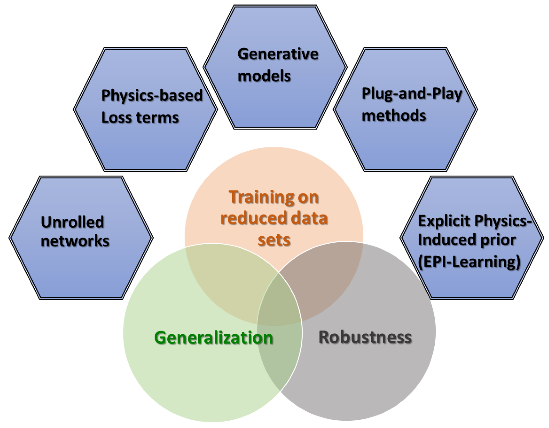
27]. Such an approach, where the physical prior is explicitly interlaced into the network architecture, may be either applied as a stand-alone model or in combination with previously introduced methods [
25,
26,
27,
28,
29], as depicted in
Figure 5. Furthermore, this would yield the potential to produce more robust and generalizable models and, hence, advance their applicability to clinical practice.


