Article

Entropy-Aware Time-Varying Graph Neural Networks with Generalized Temporal Hawkes Process: Dynamic Link Prediction in the Presence of Node Addition and Deletion

by
Bahareh Najafi
1,2,*,
Saeedeh Parsaeefard
3 and
Alberto Leon-Garcia
2
1
Department of Computer Science, University of British Columbia, Vancouver, BC V6T 1Z2, Canada
2
Department of Electrical and Computer Engineering, University of Toronto, Toronto, ON M5S 3G8, Canada
3
Apple Inc., San Francisco, CA 95014, USA
*
Author to whom correspondence should be addressed.
Mach. Learn. Knowl. Extr. 2023, 5(4), 1359-1381; https://doi.org/10.3390/make5040069
Submission received: 10 July 2023 / Revised: 10 September 2023 / Accepted: 14 September 2023 / Published: 4 October 2023

Abstract

:
This paper addresses the problem of learning temporal graph representations, which capture the changing nature of complex evolving networks. Existing approaches mainly focus on adding new nodes and edges to capture dynamic graph structures. However, to achieve more accurate representation of graph evolution, we consider both the addition and deletion of nodes and edges as events. These events occur at irregular time scales and are modeled using temporal point processes. Our goal is to learn the conditional intensity function of the temporal point process to investigate the influence of deletion events on node representation learning for link-level prediction. We incorporate network entropy, a measure of node and edge significance, to capture the effect of node deletion and edge removal in our framework. Additionally, we leveraged the characteristics of a generalized temporal Hawkes process, which considers the inhibitory effects of events where past occurrences can reduce future intensity. This framework enables dynamic representation learning by effectively modeling both addition and deletion events in the temporal graph. To evaluate our approach, we utilize autonomous system graphs, a family of inhomogeneous sparse graphs with instances of node and edge additions and deletions, in a link prediction task. By integrating these enhancements into our framework, we improve the accuracy of dynamic link prediction and enable better understanding of the dynamic evolution of complex networks.

1. Introduction

Across diverse applications, machine learning has demonstrated transformative potential, from optimizing assisted living environments [1] to innovating multilingual heritage management [2]. Within this expansive landscape lies a specific challenge: the representation learning on dynamic graphs. These graphs are prevalent in sectors such as transportation, communication infrastructure, and biological networks. These graphs provide temporal-structural information on nodes and edges, depicting the evolutionary paths of the network over time. This evolution involves the expansion and shrinkage of the network, corresponding to the addition and removal of nodes and edges. The sequences of structural changes, referred to as “events”, often occur irregularly. Extracting valuable information from such sequences of irregular past events requires modeling correlated structures between events. The temporal point process (TPP) is one of the widely used models for predicting future events based on the dependence in event occurrences [3].
The TPP is a stochastic process that describes the occurrence of discrete and asynchronous event sequences. It captures the dependencies among observations, which is crucial for accurately predicting the most likely upcoming event given the historical context. However, existing efforts for dynamic graphs primarily focus on addressing the insertion of new nodes and edges, while lacking support for deletion events due to the scarcity of publicly available datasets with fine-grained timestamps of deletion events. Incorporating deletion events necessitates more complex models. Thus, our research aims to address this gap by focusing on data-driven learning of the conditional intensity function of the temporal point process. Furthermore, we investigate network entropy as a crucial characteristic of complex evolving networks and examine the impact of node removal on entropy and other structural features of the network’s nodes and edges. We introduce latent variables that capture the effect of structural evolution in the network, enhancing the representation power of the model and providing deeper insights into the impact of node and edge removals. Our approach also considers the cooperative and interdependent behavior of addition and deletion processes in autonomous system graphs, where the addition and removal of nodes and edges are essential for maintaining connectivity. Furthermore, we conduct correlation analysis between two temporal point processes, each associated with one event type (addition and deletion). Our observations reveal that the two types of events exhibit repulsion toward each other, which can result in events inhibiting the occurrence of each other.
To take this into consideration, we leverage the generalized version of the temporal Hawkes process to model the dependencies and correlations between the two types of events. We propose our Entropy-Aware Time-varying Graph Neural Networks with Generalized Temporal Hawkes Process (Entropy-Aware GTHP-GNN) for representation learning on dynamic graphs. Our approach enhances the understanding of the influence of structural changes on network representation and enables accurate prediction of upcoming events based on the historical context. To the best of our knowledge, this work presents one of the few comprehensive studies that consider the effect of both node and edge deletions in graph representation, providing valuable insights into the dynamic behavior of complex networks. To the best of our knowledge, this work is one of the few that considers the effect of node and edge deletion processes on graph representation concisely.
The rest of this paper is organised as follows: Section 2 focuses on related approaches used for representation learning in continuous-time dynamic graphs. The concept of temporal point processes is discussed in detail in Section 3. The measurement of network entropy and its significance in the analysis of continuous-time dynamic graphs is explored in Section 4. This section thereafter enumerates the artificial characteristics of nodes and edges, including structural and statistical features, that are incorporated in representation learning.
Section 5 formulates the problem statement for representation learning on dynamic graphs. The use of GNN-based Hawkes processes for node representation learning is discussed in Section 6, along with the concept of generalized Hawkes processes. Section 7 introduces the Entropy-Aware Time-Varying GNN with Generalized Temporal Hawkes Process (Entropy-Aware GTHP-GNN) for representation learning. The performance evaluation of the Entropy-Aware GTHP-GNN is conducted in Section 8, including the challenges and limitations encountered during training. The Section Acknoledgments acknowledges the contributions and support of collaborators who have played a significant role in the research. Finally, Section 9 concludes the paper. In addition, the impact of node removal on network structural and positional features is investigated in Supplementary Material.SA. Then, in Supplementary Material.SB, the correlation analysis between two temporal point processes using the Ripley K function is presented.

2. Related Works

Graph Neural Networks (GNNs) have emerged as a pivotal tool for representation learning in graph structures, especially within the realm of dynamic networks. It is imperative to highlight that dynamic graphs can primarily be bifurcated into Discrete-Time Dynamic Graphs (DTDGs) and Continuous-Time Dynamic Graphs (CTDGs). The former are characterized by sequences of static graph snapshots, whereas the latter epitomize sequences of interactions transpiring over continuous intervals. The intrinsic capability of CTDGs to encapsulate nuanced temporal patterns has fostered the evolution of specialized machine learning paradigms, most prominently, the Temporal Graph Neural Networks (TGNNs) [4,5,6,7]. Through the strategic encoding of graph data into temporally-aware node embeddings, TGNNs exhibit a pronounced advantage over traditional GNNs, particularly in domains such as link prediction [8] and dynamic node classification [4].
Within the diverse ecosystem of GNN models, TGAT [9] has been recognized for its proficiency in decoding temporal dependencies inherent in continuous-time graphs. This model employs sophisticated attention mechanisms, enabling it to discern node interactions spanning disparate temporal phases, thereby ensuring efficient information propagation and assimilation. Contrarily, DyREP [10] adopts an approach wherein each significant event, be it the inception or dissolution of a link, is treated as a distinct training exemplar. However, this model, tailored predominantly for social network contexts, exhibits limitations, especially in datasets such as GitHub, where historical records of communication events are sparse. Furthermore, a palpable shortcoming lies in its inability to adapt its representations in response to time-varying node or edge features.
Augmenting the landscape, models such as the Latent Dynamic Graph (LDG) [11] endeavor to refine the existing architectures. They leverage the Neural Relational Inference (NRI) model [12], aiming to enhance the efficacy of self-attention mechanisms. Concurrently, another investigative work [13] harnesses the Hawkes process, emphasizing the modeling of dynamic link additions, with a concentrated focus on their temporal evolution. Conversely, FDGNN [14] introduces an avant-garde framework dedicated to node and edge embeddings. This method showcases proficiency in capturing Temporal Point Processes, hinting at the potential for devising encodings symbiotic with incoming graph events. Nevertheless, a comprehensive evaluation of FDGNN’s efficacy remains an open avenue, especially concerning the nuanced details of the node and edge attributes it seeks to incorporate.
Table 1 presents a comparative analysis of recent approaches in dynamic representation learning utilizing temporal point processes.

3. Temporal Point Process

A temporal point process is a stochastic process consisting of a time series of events occurring in continuous time [16]. They are utilised to describe data localised at a finite number of time points. The conditional intensity function of a point process is a practical and intuitive method for describing how the present in an evolutionary point process is dependent on the past. The function can be intuitively interpreted as follows:
λ ( t ) d t = [ N ( [ t , t + d t ] ) | H t ¯ ] ,
where H t ¯ is the event history up to time t, [ t , t + d t ] and N ( [ t , t + d t ] ) represent an infinitesimal time interval and number of events/points occurring in this interval. It is noted that we assume we have a simple point process, i.e., a point process in which no points coincide and the points can be ordered strictly in time. The first step in formulating a conditional intensity model for a point process is identifying the covariates that can affect the occurrence times of the process. It has been proven that the history of previous events often plays a significant role in predicting when the next event will occur. This category of covariates should be considered in the majority of point process models. If the point process being modeled is part of a larger collection of interacting point processes, it may be beneficial to consider the event histories of the other point processes in the model. In several experiments involving historical event data, additional signals or external covariates affect the point process in addition to historical terms [17].
Covariates in TPP models can affect the timing of events and are typically categorized into two types: internal and external covariates. Internal covariates, often known as endogenous covariates, are derived from the historical event data itself. The timestamps of past network events, inter-event durations, and event order are typical internal covariates. These provide insight into the intrinsic dynamics of the network event series, capturing any underlying autoregressive patterns or temporal dependencies.
External covariates, or exogenous covariates, originate outside the event series and provide additional context. These could include variables such as network load, external network events, or other observational data related to the event process but not directly part of it. For instance, in analyzing a communication infrastructure network (the event series), an external covariate could be a major external data traffic event happening at the same time.
The identification and inclusion of relevant covariates are crucial in building an effective TPP model.

4. Network Entropy

Network entropy quantifies the amount of information encoded within the structure of a network. Existing methods, including the approach proposed in [18], leverage structural information to evaluate node importance. However, instead of focusing on local connectivity patterns, network entropy captures the global attribute of the network structure. One entropic metric, called Entropy Variation, assesses the change in network entropy before and after the removal of a node. The underlying assumption is that removing a node with higher importance leads to a greater structural change.
Shannon entropy is defined as follows:
H p = i = 1 N P i log P i
For a graph G with an information function g, the graph entropy H g ( G ) is computed using probabilities derived from g. In our case, we consider second-order degree, node betweenness centrality, and edge betweenness centrality as the information functions. Consequently, we define the graph entropy based on second-order centrality as:
H D r ( G ) = i V P i log P i = i V D r [ i ] i D r [ i ] log D r [ i ] i D r [ i ] ,
where D r is the normalized second-order degree matrix.
Similarly, we compute the entropies based on node betweenness centrality ( C v B E T ) and edge betweenness centrality ( C e B E T ) as:
H C v B E T ( G ) = log i V C i B E T i V C i B E T j V C j B E T log ( C i B E T ) ,
H C e B E T ( G ) = log i E C i B E T i E C i B E T j E C j B E T log ( C i B E T ) ,
where E is the number of edges in the graph.
Entropy Variation ( E V ( v ) ) measures the change in entropy when a node v and its connections are removed from the graph. It characterizes the node’s influence on the graph structure and its significance. The modified graph after removing node v is denoted as G v ¯ .
Entropy Variation provides higher resolution compared to the initial centrality measures, as it captures more structural information and provides a global view of the connection pattern. However, computing Entropy Variation incurs higher computational complexity compared to traditional centrality metrics. Although the execution time can be reduced through parallel computing, it is important to note that the responses to node removal vary across different systems. Furthermore, the importance of nodes in complex networks is context-dependent, making it challenging to define a universal index for node importance [19].
After conducting deep investigations and running several experiments (please refer to Supplementary Material.SA for more details), we have selected the following node and edge features to reflect the important structural changes that are imposed by the deletion of nodes and edges in the graph.
Node features: node betweenness centrality ( C V B E T ), entropy variation based on node betweenness centrality ( E V C v B E T ), second-order degree ( D r ( v ) ), clustering coefficient ( C v ), standard deviation of the underlying features of immediate neighbors of v within the interval of [ t Δ t , t + Δ t ] which are cluster members m v ( t ) of v, node spectral embedding, normalized number of deletion type events at time t ( n l v ( t ) | l = 1 ), total number of deletion type events associated to node v up to time t ( t = 0 t n l v ( t ) | l = 1 ).
Edge features ( s uv ( t ) ): edge betweenness centrality ( C e B E T ), degree correlation (r).
Degree correlation: Recent research has revealed that [20,21,22] the degrees at the end of any given edge in real networks are typically not independent, but positively or negatively correlated with one another which is known to exhibit assortative and disassortative correlation mixing by degree, respectively.
Comparing different types of real networks reveals the interesting observation that the majority of social networks appear to be assortatively mixed, whereas the majority of technological and biological networks appear to be disassortative. Assortativity coefficient r within the range [ 1 , 1 ] can be used to quantify the level of degree correlation as follows.
r = M 1 e v e · u e [ M 1 e v e + u e 2 ] 2 M 1 e ( v e 2 + u e 2 ) [ M 1 e v e + u e 2 ] ,
where v e and u e represent the degrees of the nodes at the ends of the eth edge, with e = 1 , , M [23]. This formula yields r > 0 ( r < 0 ) when the corresponding network is positively (negatively) correlated, and r = 0 when no correlation [24]. The results of the underlying study indicate that node deletion results in disassortative mixing by degree in evolving networks. It is noted that the underlying research is aimed at investigating probabilistic models that explain the effects of node deletion on network structure. Such models assume a constant probability for addition and deletion of nodes and edges.
Edge betweenness centrality: Betweenness centrality of an edge e is the sum of the proportion of all-pairs shortest paths that traverse through that edge:
C e B E T = u , v V σ ( u , v | e ) σ ( u , v ) ,
where V is the set of nodes, σ ( u , v ) is the number of shortest-u,v path, and σ ( u , v | e ) is the number of those paths traversing edge e [25].
If the graph breaks down into multiple components or the number of connected components changes after a node is removed, denoted by σ G v ¯ , we can consider another node feature integrated into our model 1 σ G v ¯ σ G . The higher the underlying coefficient would be, the more structural change would be imposed to the graph after removal of node v. We will not add such a feature to our model at this point, since the AS-733 and AS-Oregon-2 graphs are perpetually connected.
Statistical features: To gain a deeper insight into the structure and dynamics of our graph data, we delve into the significance and correlations of various node features in this section. A key focus is on the latent variables we introduced to capture the structural evolution of the graph and the statistical aspects of nodes.
We introduced a set of latent variables that augment our model. These encompass indicators of the structural evolution of the graph. They include metrics such as the number of events per event types for a node v at the current time, represented as n l v ( t ) , and the cumulative events up to time t, given by t = 0 t n l v ( t ) , where l { 0 , 1 } . This concept is inspired by the survival process, where the survival rate at time t is effectively the count of nodes that have persisted until t.
Further, our analysis revealed a substantial correlation between event-based statistical features and the preceding class of node features. This observation emphasizes the relevance of the structural information from a node’s immediate neighbors at each timestamp. Consequently, each node was treated as the cluster center c v , and its connected nodes at time t were identified as cluster members m v ( t ) . The variance of the member features was then incorporated into the node features.

5. Problem Formulation

Before diving deeply into the details of our model, we provide some background on prior work in dynamic graphs using TPP.
Consider a continuous time dynamic graph G t as illustrated in Figure 1 with a set of nodes V that is represented through a static graph G t 0 (initial state of the graph at time t 0 ) along with a set of observations/events P in the form of ( u , v , l , t e ) where u , v V ( t ) are the nodes involve in the event type l. l = 0 and l = 1 represent node/edge addition and node/edge deletion, respectively, and t e is the timestamp of the event.
The dynamic graph is also denoted by a sequence of adjacency matrices A ( t ) , where A u v ( t ) denotes undirected edge from node u to v at time t. Also, we define nodes’ feature set as X ( t ) = { x v ( t ) , v V ( t ) } where x v ( t ) is the feature vector associated to node v at time t. In scenarios where the edge features are available, another set is defined as S ( t ) = { s u v ( t ) , u , v V ( t ) , u v E ( t ) } , where s u v ( t ) is the feature vector associated with edge u v in time t. A node embedding function can be represented as f :   V ( t ) Z ( t ) , which maps a given node v to d-dimensional vector z at time t, where Z ( t ) = { z v ( t ) , v , t V ( t ) , T } , z v ( t ) R d .
We consider addition and deletion as two different event types. We use l to abstract the nonlinear association between two point processes modeling addition and deletion, as inspired by [10]. Although both event types represent topological changes, they exhibit different behavior in the nature of their effect on network representation enumerated as following;
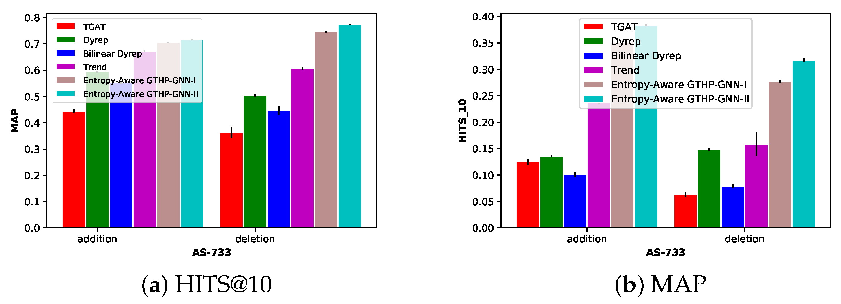
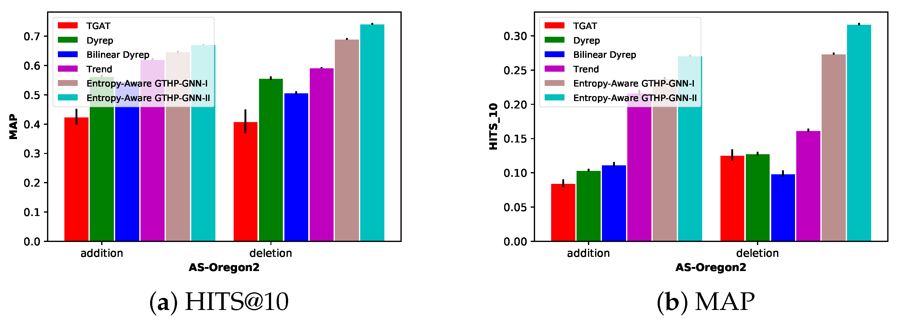
  • They occur at a very different rate. For instance, in Autonomous System graph Oregon-2 (AS-Oregon-2) [26], deletion events comprise more than 70% of the total events in the entire dataset, whereas in AS-733 number of addition types is significantly larger than the number of deletion types.
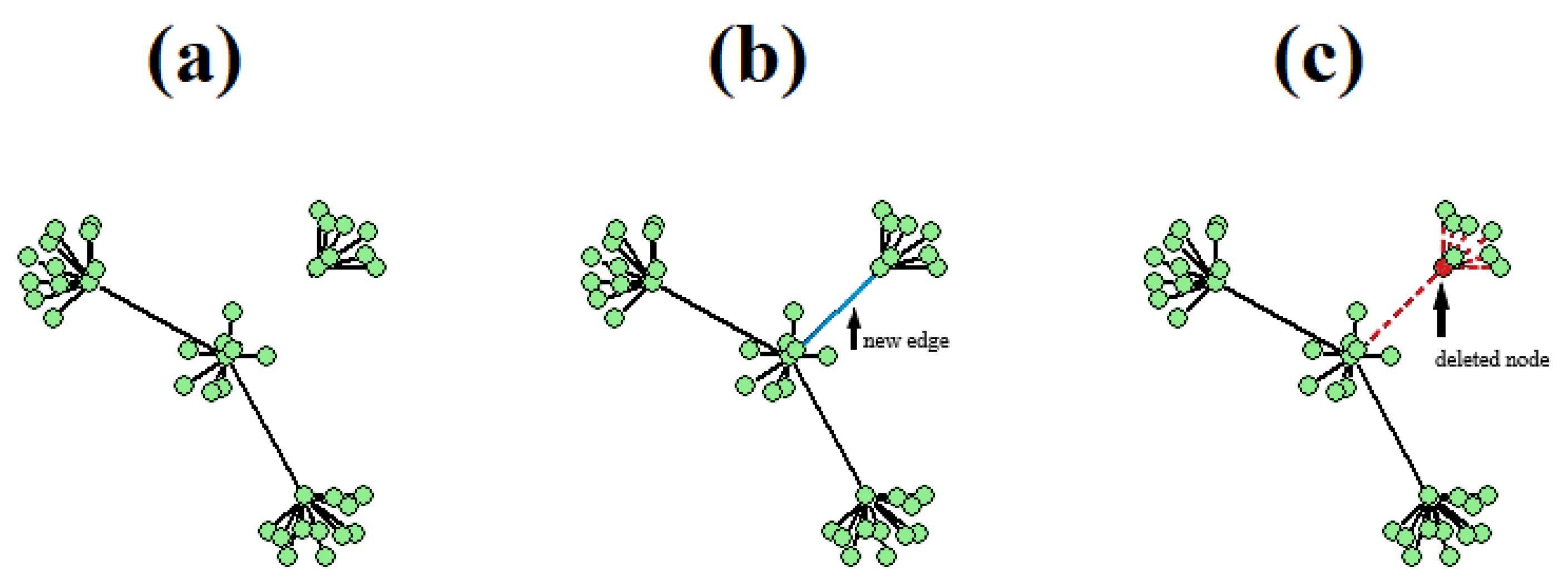
  • Deletion of a node leads to the immediate removal of all the corresponding edges that the node used to connect to its neighbors, which may ultimately lead to breaking the graph to more than one isolated subgraph. This is not the case in addition event type, in which the new node does not instantly form a certain number of new edges.
  • In many networks, the graph needs to be continuously connected and should thus respond adaptively to the combined effect of deletion and addition events by forming extra edges to maintain connectivity. For instance, in AS-733 dataset [26], for few selected subgraphs the graph is multiple nodes’ removal away from being disconnected. This explains why there are far more addition event types than deletion event types.
The conditional intensity function λ l u , v ( t ) describes the probability of the occurrence of an event between v and u in an infinitesimal time interval ( t , t + d t ] . Our focus is to learn the conditional intensity function of the temporal point process in a data-driven manner. The first step in formulating a conditional intensity model for a point process is identifying the covariates that can affect the occurrence times of the process. It has been proven that the history of previous events often plays a significant role in predicting the timing of the next event. This category of covariates should be considered in the majority of point process models. If the point process being modeled is part of a larger collection of interacting point processes, it may be beneficial to consider the event histories of the other point processes in the model. In several experiments involving historical event data, additional signals or external covariates affect the point process in addition to historical terms [17].
We define a model for λ as a function of covariates that can influence the occurrence and timing of the events. Additionally, we model our point process as a larger collection of two point processes that interact with each other. Our goal is to make a prediction through frequently updating representation of nodes, z v ( t ) , involved in the events. This update is being applied right after the occurrence of each event of both types ( l { 0 , 1 } ). So, z v ( t ) is the outcome of the influences that several covariates made on the involving nodes and it is also reflective of how irregular sequence of past events affected the representation of node v. Therefore, we define conditional intensity as λ l u , v ( t ) = f l ( g l u , v ( t ) ) , where g l u , v ( t ) is calculated as in g l u , v ( t ) = ω l τ · [ z u ( t ¯ ) , z v ( t ¯ ) ] , where z v ( t ¯ ) and z u ( t ¯ ) are the most recent embedding vectors of nodes v and u, respectively. Here, we design the function f as below (see Figure 2):
f l ( x ) = 2 x ( Φ ( ψ l · x ) 1 2 ) ,
where Φ is the cumulative density function of the standard Gaussian distribution. ψ l is a learned parameter specified to event type l. The function has the following characteristics: (I) It is positively differentiable, (II) strictly increasing, and (III) its oblique asymptote is the identity function. This choice of f l has considerably improved the performance compared to the modified softplus version used in the literature [27] ( f l ( x ) = ψ l · log ( 1 + exp ( x ψ l ) ) ). Figure 2a illustrates the outcome of the proposed activation function in (6) under several trained values of ψ . Figure 2b shows the ratio of the underlying function to the widely used scaled softplus function. The ratio approaches line y = 1 with different slopes for all trained values of ψ .

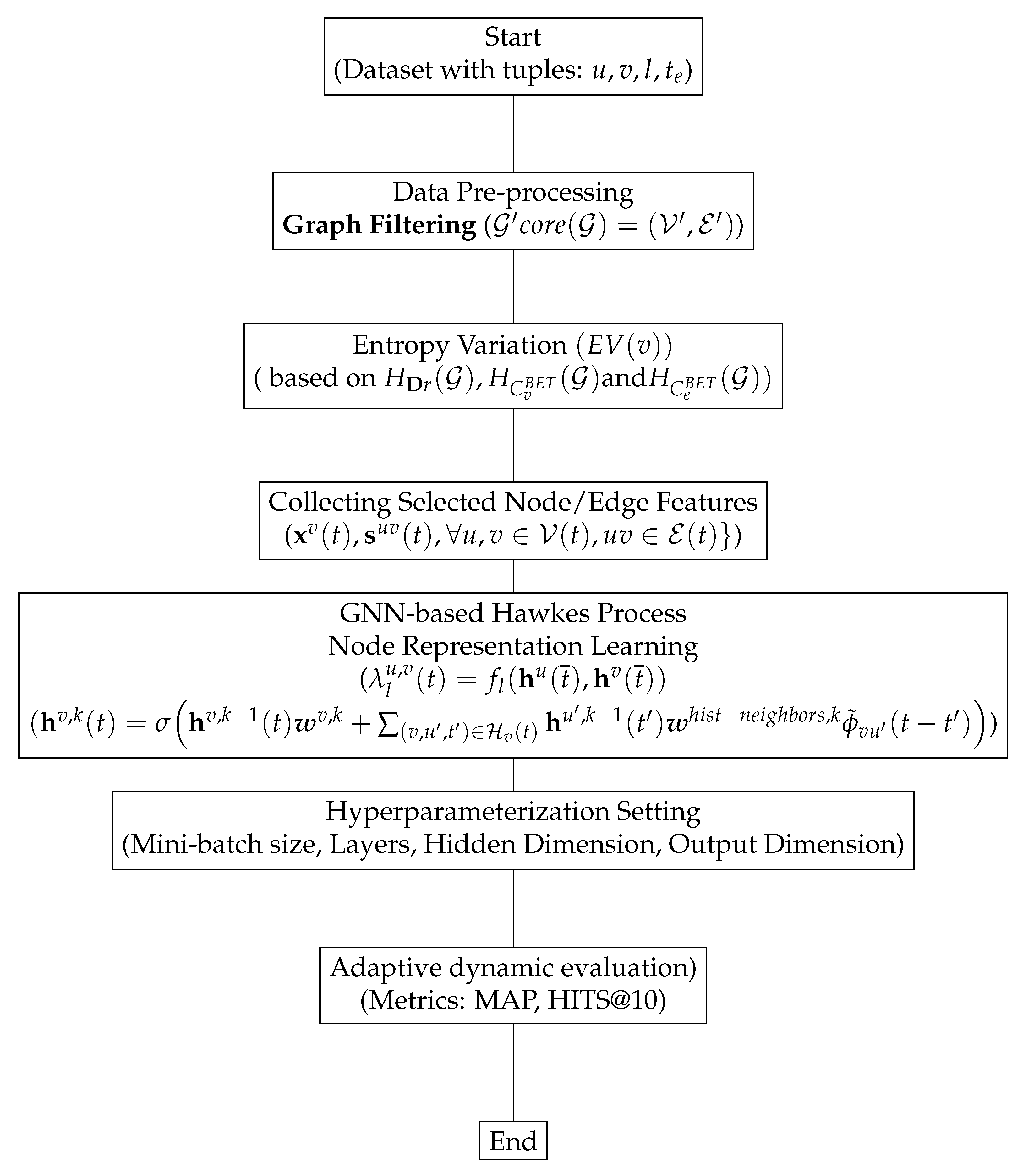
6. GNN-Based Hawkes Process for Node Representation Learning

In this section, we discuss the critical issue of temporal graph representation learning using Hawkes process, in which we acquire representations that change over time on a graph. We consider the formation or removal of a link at a specific time to be an event, and a graph evolves continuously as more events are added [28].
In general, temporal graph representation learning requires that the learned representations not only preserve graph structures and node features, but also reflect the graph’s topological evolution. This goal, however, is not trivial, and several works on the subject have only recently emerged. To simplify the model, some studies [29,30,31,32] discretize the temporal graph into a series of static graph snapshots. As a result, they are unable to fully capture the continuously evolving dynamics, because the fine-grained events between the snapshots are inevitably lost. CTDNE [33] uses temporal random walks that respect the chronological sequence of the edges for continuous-time methods, whereas TGAT [9] maps continuous time and self-attention to aggregate temporal-topological neighborhood using a GNN framework with functional time encoding. These methods, however, frequently fail to capture the exciting/inhibiting effects [34] between sequential events, particularly the influence of historical events on current events. Nonetheless, such effects can be captured well by temporal point processes, most notably the Hawkes process [27,35], which assumes that historical events prior to timestamp t can excite the process in the sense that future events become more likely for some time after t. This property is useful for simulating the graph-wide addition/deletion process, in which each link formation/removal is viewed as an event that can be triggered by recent events. However, conventional Hawkes process-based network embedding techniques [34,36] are intrinsically transductive, making them unsuitable for learning temporal graph representations. In contrast to our framework in this paper, DyRep [10] and Trend [13] propose an inductive framework based on the temporal point process and Hawkes process, respectively, restricting their framework to network growth; only the addition of new nodes and edges is considered. On the other hand, with respect to Dyrep, the model updates the representation of participating nodes one by one after the occurrence of each event. By giving the overall history of all events with respect to a given node at time t, the model would have learned the correlation among the events and the other end of the communication link in terms of common associated structural features and would perform better in terms of predicting the most likely nodes that have been involved in an event with the underlying given node in the future.

Generalized Hawkes Process

The Poisson process [37], which implies that events occur independently of one another, is a fundamental model for event streams. In a non-homogeneous Poisson process, the (infinitesimal) chance that an event will occur at time t may fluctuate with time t, but it remains independent of previous occurrences. A Hawkes process, however, assumes that past events might temporarily increase the likelihood of future events, given that such excitation is (I) positive, (II) additive over past events, and (III) exponentially fading over time.
However, it appears that real-world patterns frequently contradict these assumptions. For instance, rule I is violated when one event inhibits rather than stimulates another, like when cookie consumption inhibits cake consumption. When the cumulative effect of prior occurrences is not additive, rule II is violated [27]. In addition, III is violated when, for instance, a prior event has a delayed effect such that the effect begins at 0 and rapidly increases before declining [27]. By generalising Hawkes, our model is able to account for impacts that the Hawkes procedure overlooks. As such, the effect of previous events on future events might be superadditive, subadditive, or even subtractive, depending on the order of the past events. Before introducing our model, we briefly study Hawkes processes below.
The non-homogeneous Poisson process is a fundamental model of event streams. It posits that an event of type l occurs with probability λ l ( t ) d t at time t, more precisely in the infinitely large interval [ t , t + d t ) . Similar to the parameter of an ordinary Poisson process, the value λ l ( t ) 0 can be interpreted as a rate per unit time.
The self-exciting point process or Hawkes process [35] is a well-known generalisation that captures interactions. In this model, historical events combine to increase the intensity of each type of event. This stimulation is positive, cumulative to past events, and decays exponentially with time as below:
λ l v ( t ) = μ l v ( t ) + u = 1 N t l u < t α l u v exp ( δ l u v ( t t l u ) ) ,
where μ l v ( t ) 0 is the base intensity of event type l corresponding to node v, α l u v is the degree to which an event of neighbor node u with type l initially excites type l event for node v and δ l u v > 0 is the decay rate of excitation. When an event occurs, all intensities increase to varying degrees, but subsequently return to their baseline μ .
Hawkes process expressivity is constrained by positive constraints. First, the positive interaction parameters α u v fail to account for inhibitory effects, in which previous events diminish the intensity of future occurrences. Second, the positive base rates μ v fail to account for the inherent inertia of certain events, which are unlikely until their cumulative stimulation by previous events exceeds a certain threshold. In order to eliminate such constraints, we use generalised Hawkes process in which intensity λ v ( t ) can even fluctuate between successive occurrences, as excitatory and inhibitory influences might dissipate at different rates. This allows inhibition δ l u v < 0 and inertia μ l v < 0 to occur. Nonetheless, the total activation may now be negative. Therefore, we pass it through a nonlinear transfer function f l in order to generate the requisite positive intensity function: λ ˜ l v ( t ) = f l ( λ l v ( t ) ) . It is noted that the intensity λ may both increase and decrease over time, but the influence of each preceding event continues to decay toward 0 at a rate δ u v > 0 . With respect to the choice of nonlinear function f l , we use a variant of scaled softplus with a separate event type specific scale parameter and another designed GELU-based transfer function that we previously discussed.
Now, we propose our Generalized (with inhibition) Temporal Hawkes process-based GNN for dynamic graphs. Previous techniques do not use Hawkes or similar point processes to simulate the combination of exciting and inhibiting effects between events [9,13], message-passing GNNs to preserve the structures and characteristics of nodes in an inductive fashion [34,36], or any of those [33]. Note to add: please talk about attributed graph and very few works that considered node attributes and how node structure can affect the node representation over time.
On the other hand, although events have individual features, they are rarely created in isolation, and events that are related frequently have communal traits. Events that share a node can be viewed as a cluster due to their shared neighbor node’s common effect. That is, the cluster of events for each node should correspond to its rate of occurrence, Obviously, each node would have its own event cluster, and each cluster would correspond to the varied rate of occurrence of the two nodes. In addition, as the graph evolves throughout the time, a node’s tendency to connect with other nodes (e.g., previous neighbors) would change. In other words, the events emanating from a shared node are governed in a group by the ’node’s dynamics’ [27] as a function of time. Consequently, in order to model the communal properties of events originating from the same node, we consider the common node as the cluster center and compute the standard deviation of the highly influencing features of the underlying node’s neighbor at the time and integrate them into our model as the node’s dynamic features.
In the previous section, we introduced the temporal Hawkes process and its generalized form in discrete time. In its continuous-time form, the Hawkes process [36] is defined as follows:
λ ( t ) = μ ( t ) + 0 t ϕ ( t t ) d N ( t ) ,
where ϕ ( t ) is a kernel function that models the decay of previous events’ influence on the current event, and N ( t ) is the number of occurrences up to time t. Given the characteristics of the generalized Hawkes process, it is particularly suited for modeling the graph-wide structural evolution process in a dynamic graph because it can represent the influence of historical events as a whole by simulating the stimulating (exciting and inhibiting) effects between events.

7. Entropy-Aware GNN-Based Generalized Temporal Hawkes Process for Dynamic Link Prediction

In Section 6, we introduced the temporal Hawkes process and its generalized form in discrete time. In its continuous-time form, the Hawkes process [36] is defined as follows:
λ ( t ) = μ ( t ) + 0 t ϕ ( t t ) d N ( t ) ,
where ϕ ( t ) is a kernel function that models the decay of previous events’ influence on the current event, and N ( t ) is the number of occurrences up to time t. Given the characteristics of the generalized Hawkes process, it is particularly suited for modeling the graph-wide structural evolution process in a dynamic graph because it can represent the influence of historical events as a whole by simulating the stimulating (exciting and inhibiting) effects between events.
Built upon a Hawkes process-based GNN, the proposed model is capable of inductively modeling the structural evolution process (addition and deletion of nodes and edges) of the graph. Moreover, the model incorporates entropy-aware structural and event-based statistical features to reflect the effects of graph growth and shrinkage on node representation learning. The GNN layer aggregates the node feature information with the features from previous neighbors to materialize the generalized Hawkes conditional intensity.
We start with the presentation of a GNN framework based on generalized Hawkes processes. The formation/removal of links across a graph can be modeled by the generalized Hawkes process. To be more precise, the conditional intensity of the event can be used to quantify whether or not nodes u and v form a link at time t.
λ l u , v ( t ) = μ l u , v ( t ) + ( u , v , t ) H u ( t ) α l v ( t ) ϕ l ( t t ) + ( u , v , t ) H v ( t ) α l u ( t ) ϕ ( t t ) ,
where H u ( t ) = { ( u , v , t ) N u ( t ) : t < t } is the set of historical events of type l which nodes u and v each had with their previous one-hop neighbors. α l v ( t ) denotes the degree of which the previous event of historical neighbor v with event type l at time t excites or inhibits the current event. The exponential function ϕ l ( t t ) = exp ( δ v ( t t ) ) is a kernel function used to represent the time decay effect with learnable rate δ of the underlying historical neighbors with respect to u up to time t. As can be seen, both parameters α l v ( t ) and μ l u , v are event type (l) specific. It is noted that we are working with undirected graphs. As a result, the current event is influenced by the previous neighbors of both involving nodes u and v.
Temporal GNN Layer: By virtue of their inductive nature and superior performance, GNNs serve as the materialization mechanism for the temporal representations in ( λ l u , v ( t ) = f l ( h u ( t ¯ ) , h v ( t ¯ ) ) ). Each node in a multi-layered network uses the message-passing scheme to recursively receive messages (features or embeddings) from its neighbors (nodes and/or edges) and aggregate them with dynamic features of its own. We present a temporal formulation of GNN that makes use of the learned temporal representations to materialize the conditional intensity function of the Hawkes process. The d-dimensional embedding vector of node v at time t in layer k is as follows:
h v , k ( t ) = σ ( h v , k 1 ( t ) w v , k + ( v , u , t ) H v ( t ) h u , k 1 ( t ) w h i s t n e i g h b o r s , k ϕ ˜ v u ( t t )
The first component, h v , k 1 ( t ) w v , k is analogous to the base intensity in (10) which is only dependent on the self-node representation. The second component, on the other hand, aggregates the feature information of the historical neighbors, which is aimed to capture the inhibition/excitement caused by previous events. σ is the activation function; w v , k and w h i s t n e i g h b o r s , k are the learnable weight matrices that map the representation of the self node and its historical neighbors from the previous layer, k 1 , respectively. ϕ ˜ v u ( t t ) captures the effect of time decay based on the time kernel with softmax, which is defined by ϕ ˜ v u ( t t ) = exp ( δ v u ( t t ) ) ( v , u , t ) H v ( t ) exp ( δ v ( t t ) ) . The node dynamic representation at time t in the last layer is given by h v ( t ) .
Complexity Analysis: The complexity of the Entropy-Aware GTHP-GNN algorithm is primarily determined by two main operations: the computations in the GNN layers and the backpropagation during the training process.
Firstly, let us consider the GNN layer computations. For each GNN layer, a node v receives and aggregates messages from its historical neighbors, as represented in H v ( t ) . This process needs to be performed for each node in the graph, leading to a time complexity of O ( | H v ( t ) | · | V | · d · k ) , where | V | is the number of nodes in the graph, d is the dimension of the node embeddings, | H v ( t ) | is the number of historical neighbors for a node, and k is the number of GNN layers.
During backpropagation, the gradient of the loss function is calculated and used to update the parameters of the model. The time complexity for this operation is roughly O ( T · m ) , where T is the total number of time steps and m is the number of parameters in the model. Thus, the overall time complexity of the Entropy-Aware GTHP-GNN algorithm can be approximated as O ( | H v ( t ) | · | V | · d · k + T · m ) .
Convergence Behavior: The convergence of the Entropy-Aware GTHP-GNN algorithm is considered reliable due to the characteristics of the optimization process and the nature of the GNN model.
Given that the GNN layer computations and backpropagation process are both iterative and based on gradient descent, the model converges to a local minimum, assuming the learning rate is well-tuned.
Furthermore, the GNN’s ability to capture complex dependencies in the graph and the inclusion of entropy-aware features can guide the model towards better solutions, improving the convergence behavior. However, it is also crucial to note that the algorithm’s convergence speed could vary depending on factors such as the learning rate and the size and quality of the input data.

8. Performance Evaluation

Figure 3 illustrates the end-to-end process. We investigate the performance of our framework by assessing our model on the dynamic link prediction task. To achieve this, we formulate the following question: “At time t, which node u is most likely to be involved in an event of type l with a given node v?” We address this problem using the conditional density function as computed in [10]:
f l u , v ( t ) = λ l u , v ( t ) · exp ( t ¯ t λ ( r ) d ( r ) ) , where λ is measured as described in Section 7. For a given test record ( u , v , l , t e ) , we substitute v with other entities in the graph and compute the density in the same manner as described in the previous section. Afterwards, we rank all the entities in descending order of density and report the position of the ground truth entity.
Figure 3. Flowchart of Entropy-Aware GTHP-GNN.
Make 05 00069 g003
Each experiment is repeated 10 times, and we measure Mean Average Precision (MAP) and HITS(@10) for both addition and removal types of events. We have chosen these metrics to evaluate the link prediction performance because they provide a comprehensive evaluation that considers the entire ranking list, capturing the quality of predictions at various positions. This is particularly valuable for our sparse and inhomogeneous dataset, enabling a fair comparison of different models and techniques while accounting for the ranking order and precision at each position. MAP measures the average precision of a model’s ranked predictions across all positions, providing a comprehensive assessment of the quality of the entire ranking list. Hits@10 measures the proportion of correct predictions within the top-10 ranked items, indicating the model’s ability to identify relevant items in a ranking setting, with a focus on the top positions. It also indirectly suggests the model’s stability by assessing its ability to consistently identify relevant items within the top positions.
Additionally, we adopt a dynamic train-evaluation setting inspired by [38]. This setting is proposed to address the limitation of a fixed train-validation-split setting for dynamic graphs. It continuously updates the model parameters based on historical graph snapshots and evaluates the performance on the current graph snapshot. It allows the model to adapt to the evolving graph structure and capture temporal dependencies in the data. This setting enables the model to learn from past graph instances and incorporate the latest information, improving its ability to make accurate predictions in dynamic environments. Thus, it provides a more realistic and effective approach for training and evaluating models in dynamic graph learning tasks. For more details, please refer to Algorithm 1.
Algorithm 1 Adaptive dynamic evaluation for Entropy-Aware GTHP-GNN
Input: Dynamic graph representation G ( t ) , Initial node states H 0 , Node features x v ( t 0 )
Output: Updated node state representation H ( T ) , Mean average precision MAP
  1:
Initialize hierarchical node state  H 0  with the set of node features  x v ( t 0 )
  2:
for  t = 2  to T do
  3:
     Collect target labels  target ( t 1 ) = target ( t 1 ) target val , target ( t )
   4:
    while MAP ( t 1 ) is increasing do
  5:
          H ( t 1 ) , target_hat ( t 1 ) Entropy-Aware GTHP-GNN ( G ( t 1 ) , H ( t 2 ) )
  6:
          target _ hat ( t 1 ) target _ hat ( t 1 ) target _ hat val
  7:
         Update Entropy-Aware GTHP-GNN via backpropagation based on  target _ hat ( t 1 ) , target ( t 1 )
  8:
         MAP ( t 1 ) Evaluate ( target _ hat ( t 1 ) , target ( t 1 ) )
  9:
     end while
10:
      H ( t ) , target _ hat ( t ) Entropy-Aware GTHP-GNN ( G ( t ) , H ( t 1 ) )
11:
     MAP ( t ) Evaluate ( target _ hat ( t ) , target ( t ) )
12:
end for
13:
MAP  = t = 2 T 1 MAP ( t ) / ( T 1 )
We utilized the last 100 snapshots of the AS-733 dataset and the entire graph of AS-oregon2 for our experiments. We also performed the same pre-processing techniques discussed in Section 8.2. Figure 4 illustrates a selection from the AS-733 dataset, showcasing 20 prominent nodes, most of which are the highest degree nodes. Central nodes, defined by their high degree and often elevated node betweenness centrality, play a crucial role in the network’s architecture. Their strategic position within the network underscores their importance; their removal could potentially fragment the graph, leading to substantial disruptions in connectivity.
However, an intriguing characteristic of autonomous system graphs is their adaptive nature. Should central nodes face removal or disconnection, these graphs often exhibit a compensatory mechanism, introducing new connections to counteract the resultant disconnectivity. This resilience ensures that the network remains operative, with minimized disruptions.
On the periphery, nodes predominantly display degrees ranging from 1 to 4. This distinct disparity in node degrees—with a cluster of highly connected nodes and a larger set with minimal connections—epitomizes the properties of scale-free networks. These networks, found in diverse real-world scenarios from the Internet to biological pathways, possess unique properties that influence their robustness and vulnerability.
We evaluate the performance of our proposed model with the following benchmarks:
TGAT: TGAT maps continuous time and self-attention to aggregate a temporal-topological neighborhood using a GNN framework with functional time encoding.
Dyrep: The work introduces a novel framework for learning dynamic node representations in temporal graphs. It utilizes a memory module and a recurrent mechanism to capture the temporal dependencies and update node embeddings efficiently, achieving state-of-the-art performance on various dynamic graph tasks [10].
Bilinear Dyrep: The paper proposes a method that combines temporal attention mechanisms and bilinear interactions to model the temporal dynamics in dynamic graphs. It introduces Neural Relational Inference to improve upon the temporal self-attention mechanism in Dyrep [11].
Trend: The study utilizes the Hawkes process to model link addition in dynamic networks. It incorporates node dynamics and event estimation to capture the temporal evolution of the network [13].
Entropy-Aware GTHP-GNN-I: Our proposed method with transfer function f l ( x ) = ψ l · log ( 1 + exp ( x ψ l ) ) .
Entropy-Aware GTHP-GNN-II: Our proposed method with transfer function in Equation (6).
The two distinct transfer functions are tailored to enhance the models’ representation capabilities in different ways: For Entropy-Aware GTHP-GNN I, the function introduces a nonlinear transformation, smoothing out extreme values in the node representations. The multiplication by the parameter ψ l scales the output, and the logarithm, combined with the exponential, ensures that the function can capture rapid changes in the graph’s structure but remains stable even when x is large. This kind of function is particularly useful when dealing with graphs that exhibit rapid evolutions or significant variations in their structure, allowing the model to adapt to sudden shifts in the data while maintaining robustness.
For Entropy-Aware GTHP-GNN II, the chosen transfer function is given by f l ( x ) = 2 x ( Φ ( ψ l · x ) 1 2 ) , where Φ represents the standard Gaussian cumulative distribution function (CDF). This transfer function, built upon the CDF, inherently provides a probabilistic measure. The function takes values between 0 and 1 and modulates the input x based on how it positions relative to the Gaussian distribution scaled by ψ l . Essentially, this function can highlight or attenuate certain features in the node representations based on their relative significance or rarity. This is especially beneficial when dealing with graphs where rare connections or features can have significant importance.

8.1. Datasets

In the following section, we describe the characteristics of datasets used in our experiments.

8.1.1. Autonomous System Dataset

We choose autonomous system datasets, a communication network infrastructure dataset derived from Border Gateway Protocol(BGP) logs [26]. It is comprised of Autonomous Systems (ASes), each of which is a network with its own routing policy administered by a single authority. ASes peer to exchange traffic and use the BGP to exchange routing and reachability information within the Internet’s global routing system. The network can therefore be represented by a graph in which ASes are nodes and BPG peering relationships are links. The dataset consists of 733 daily instances spanning 785 days between 8 November 1997 and 2 January 2000. Unlike the majority of other graphs, which only have instances of node and edge addition, this graph also has instances of node and edge deletion. We use the last 100 snapshots from this dataset. Autonomous graphs are undirected, sparse graphs with irregular structural event occurrences. The graph is scale-free, with few nodes of higher-order degree and many nodes of lower-order degree.

8.1.2. AS-Oregon-2

From 31 March 2001 to 26 May 2001, nine graphs of autonomous systems were produced, one per week. AS peering information inferred from Oregon route-views, Looking glass data, and Routing registry are all combined.
Both AS-733 and AS-Oregon2 are non-attributed graphs, meaning there are no edge or node features. We adopted some structural node and edge time-varying characteristics that not only improved prediction performance but also highlighted the impact of network evolution on the graph. The underlying datasets are well-established benchmarks in network studies, offering robustness to the results. In addition, despite their age, the fundamental network evolution patterns they display remain relevant.

8.2. Data Pre-Processing
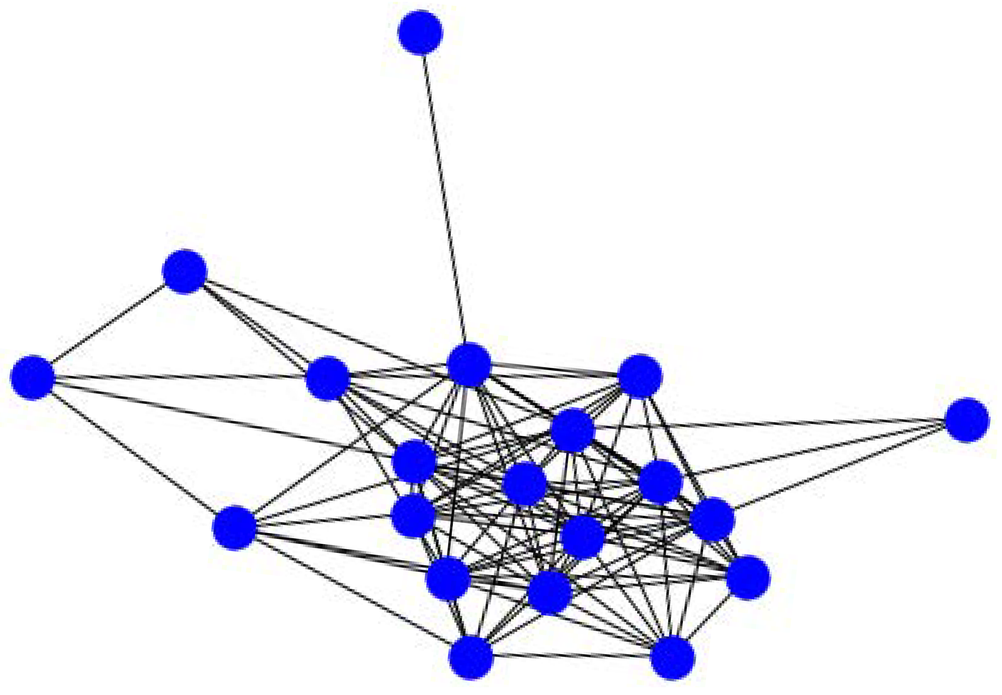
Data are reported every day in the form of a tuple (node1, node2, and timestamp) in a txt file. node1 and node2 are the start and end nodes of an event, and the timestamp is the time the event happened; self-loop and repetitive tuples are removed.
There are two event types in general: addition and deletion. Addition refers to the addition of any node, which is manifested in the form of new edges connecting the underlying new node to another new/existing node. Edge addition could also refer to the addition of a new edge between two existing nodes. Node deletion indicates the deletion of any node that is represented in the form of removal of all the edges/connections connecting the underlying node to any other node. In addition, edge removal in general could also indicate the removal of an edge only, without any end nodes being removed. To figure out the types of events, we made a list of all the nodes that were involved in all the events for a given date and compared it to the same list for the date after it. Then, we extracted the new nodes and edges that appeared in the following date, as well as the nodes and edges that were removed. We realized that all new edges are being formed between either two new nodes or one new node and one existing node in the AS dataset. Additionally, all edge deletions occurred as a result of the removal of an existing node. Following that, we labeled the events as additions and deletions. Events are reported in large batches in chronological order. Since each individual event required a timestamp, while preserving the order and the date on which an event occurred, we scattered all events of a day in a 24 h time span by sorting a set of randomly generated timestamps where each date/time was artificially assigned to an event. It is noted that the time difference between consecutive events of a given date could be in the range of a few minutes to a few hours. In the case of deletion events, we also record at the time, t c , when the new node or edge was created.
By looking at density, the AS graph is highly non-uniform. Most of the nodes simply have weak connections to one another [39]. To work around this characteristic and focus on important ASes, we use a technique called “graph filtering” which is introduced below.
Graph Filtering: The process of filtering out irrelevant information from large datasets is a fundamental step in various analyses. To this end, numerous authors have sought to identify the most relevant elements within the Autonomous System (AS) graph. A frequently used parameter is the degree of a node, as employed by Tauro et al. [40]. Taking inspiration from Gaertler et al. [41], our work makes use of the concept of coreness, which is closely related to node degree and was introduced by Seidman [42].
Coreness refers to the unique subgraph obtained by recursively removing all nodes with a degree less than a certain value, k. A node is said to have a coreness value of l if it belongs to the l-core but not to the ( l + 1 ) -core. Previous research indicates that the proportions of nodes with the lowest and highest coreness remain consistent over time, providing a reliable measure. By applying this concept, peripheral ASes can be filtered out, leading to a more simplified and meaningful representation of the network.
Key advantages of this streamlined representation include:
(I)
Prominent ASes Highlighted: By eliminating nodes with fewer connections, the focus shifts towards the influential ASes, which often play a pivotal role in network operations.
(II)
Computational Efficiency Improved: The reduction in network size enhances the computational efficiency of the graph-based algorithms employed.
(III)
Noise Reduction: In complex networks, nodes with weak or trivial connections often contribute to noise. This noise is minimized by our filtering process, thereby emphasizing the more significant connections.
The coreness concept does not interfere with the scale-free property of AS graphs, as the value of k is carefully chosen based on the number of remaining ASes, aiming for a balance between computational feasibility and meaningful network representation.
In our approach, the graph is simplified to a core graph, G c o r e ( G ) = ( V , E ) , from the original graph G = ( V , E ) . In this core graph, a node is represented for each distinct coreness value. Two nodes, u and v, are connected if there are edges incident to coreness u and v nodes in the original graph, denoted as E u , v .
To manage the heterogeneous property of AS graphs and to emphasize important ASes, we were also inspired by the geometric clustering method by Brandes and Pich [43]. This method generates a hierarchy of clusters with significant geographical ties by selecting a subset of the eigenvectors linked to the largest eigenvalues of the normalized adjacency matrix. Thus, we chose a k-core small enough that it contains no more than 600 nodes at each graph snapshot, thereby maintaining a balance between computational feasibility and meaningful network representation given the inherent characteristics of the dataset.
Hyperparameterization Setting: We conduct our experiments using the following hyperparameter settings. We utilize a mini-batch size of 16 during the training process. For all benchmarks, we set the number of layers to two, with a hidden dimension of 32 for the AS-733 dataset and 64 for the AS-Oregon2 dataset. The output embedding dimension is set to 128 for the AS-733 dataset and 64 for the AS-Oregon2 dataset. We apply the ReLU activation function after each layer. To balance the training dataset, we include one negative sample per event. In our link prediction task, we employed negative sampling to augment the positive samples. For each pair of connected nodes ( v , u ) at time t, which were considered as positive samples, we introduced negative samples ( v , w ) where the pair was not connected at time t.
The purpose of negative sampling is to create a balanced training dataset that includes both positive and negative examples. By including negative samples, the model learns to distinguish between true positive connections and false negative connections, thereby enhancing its ability to discriminate between connected and unconnected node pairs.
In our approach, we ensured that the number of negative samples per event was set to 1. This choice helped maintain an appropriate balance between positive and negative examples during training, enabling the model to effectively capture the underlying patterns and relationships within the dynamic graph data.
The results depicted in Figure 5 showcase the Mean Average Precision (MAP) and HITS(@10) scores of our method compared to four benchmarks in the link prediction task using the AS-733 dataset. Our method exhibits superior performance in both metrics, with a more substantial improvement observed for deletion events. Additionally, the benchmarks generally demonstrate higher MAP performance for addition events, potentially attributed to the higher occurrence of addition events compared to deletion events in the AS-733 dataset. This could also indicate that the models have a harder time predicting links that are about to disappear than predicting new ones.
Both the Entropy-Aware models outperformed Dyrep by significant margins in both addition and deletion scenarios. Particularly, the Entropy-Aware GTHP-GNN-II model showcased an impressive increase in MAP by +0.1234 for addition and +0.2682 for deletion. The Trend model also showed improvements over Dyrep, but to a lesser extent than the Entropy-Aware models. Bilinear Dyrep had a minor drop in performance compared to Dyrep, especially in the deletion scenario and TGAT performed below Dyrep for both operations.
Figure 6 illustrates the evaluation results of the model for the AS-oregon2 dataset under the link prediction task. AS-oregon2 is another member of the Autonomous System family, containing weekly instances from 31 March to 26 May 2001, representing AS peering information inferred from multiple views [26]. As can be seen in the plot, Entropy-Aware GTHP-GNN demonstrates better performance compared to the benchmarks. It is worth noting that the proportion of addition and deletion events differs significantly between the two datasets. In AS-733, the majority of records are additions of nodes and edges, while in AS-oregon2, the proportion is more balanced. This difference in event proportions may contribute to the observed variation in MAP performance improvement between the two datasets.
Specifically, AS-Oregon2 exhibits an average clustering coefficient (0.5) that is twice as high as that of AS-733. This significant difference suggests a greater level of local connectivity within AS-Oregon2, accompanied by the presence of more robustly connected subgraphs within the larger network. Consequently, this enhanced connectivity contributes to improved performance prediction capabilities. The clustering coefficient serves as a metric for assessing the tendency of nodes in a graph to form clusters or tightly interconnected groups, effectively capturing the density of connections among a node’s neighbors.
Both versions of the Entropy-Aware GTHP-GNN method have shown commendable improvements in MAP and Hits@10 compared to Dyrep. Their effective integration of the generalized/modified Hawkes process lets them adaptively learn the intricacies of addition events. The specific transfer functions used also assist in refining the predictions, aiding in identifying potential connections. In deletion events, the entropy-aware design ensures a robustness in recognizing dwindling connections or less active nodes, making the model more proficient in predicting deletions. One interesting aspect to highlight is the presence of error bars, which represent the standard deviation of the data. Lower standard deviation indicates that the results are more reliable and consistent. In this regard, the Entropy-Aware GTHP-GNN-II model shows the smallest error bars, which means it not only performs better on average but also delivers more stable and predictable performance.
While both entropy-aware models demonstrate strengths, Entropy-Aware GTHP-GNN II’s probabilistic approach in the transfer function might make it slightly more adept in anticipating rare addition events and consequently less adept in predicting deletions than its counterpart. These superior results can be attributed to the following pivotal factors:
(I)
Generalized Hawkes Process: Unlike some benchmark models, the Entropy-Aware GTHP-GNN models, through the generalized Hawkes process, adeptly capture the temporal intricacies within the network. This ensures that the likelihood of an event’s occurrence is substantially influenced by past events, a critical feature in dynamic networks.
(II)
Entropy Awareness: This model’s entropy-aware approach enables a deep comprehension of the evolving graph structure. By gauging the uncertainty or randomness of a node’s connections over time, the model can better predict connection trends, contributing to its high performance.
(III)
Dynamic Training: The adaptive nature of the model, which iteratively updates based on past graph snapshots and gauges performance on the most recent snapshot, bolsters its adaptability to changing graph structures and temporal dependencies.
(IV)
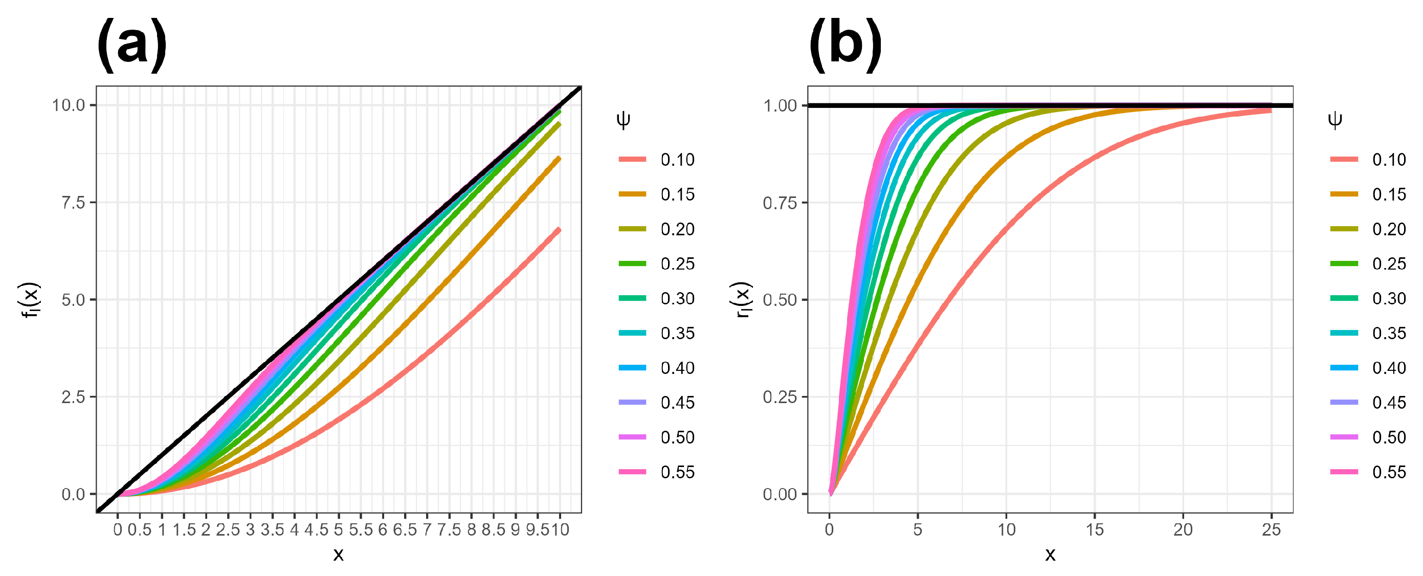
Transfer Functions: The dual approach of integrating both softmax and a creative GELU-based function accentuates the model’s versatility. While softmax offers a probabilistic classification of node connections, the modified GELU captures the complex, nuanced relationships within the graph.
The Trend model, which incorporates the Hawkes process, displayed enhanced performance over the Dyrep model. This signifies the efficacy of the Hawkes process in forecasting trends. However, the improvements exhibited by the Trend model were not as pronounced as those seen in the Entropy-Aware models.
With Dyrep, as a pioneering approach in temporal point process-based dynamic representation learning, Dyrep sets the baseline. Its strength lies in modeling the dynamic evolution of connections. However, when juxtaposed against more recent or specialized models, it might not capture the nuanced entropy changes or specific temporal dependencies as adeptly.
With respect to bilinear Dyrep, while it represents an iteration on the original Dyrep, its reduced MAP scores indicate that bilinear transformations, although useful in certain scenarios, might not have brought out significant advantages for this task or datasets.
On the other hand, TGAT consistently lags behind Dyrep, suggesting that while TGAT might be adept at handling other tasks or datasets, it might lack specific features to address the intricacies of temporal point processes in dynamic graphs.
In conclusion, these graphs provide strong evidence in favor of the Entropy-Aware GTHP-GNN-II model, given its high performance in MAP and Hits@10 and low variability in results across different types of operations (addition or deletion) and datasets.
Furthermore, it is pivotal to note that the variation in performance improvement across different datasets is influenced by their inherent characteristics. Factors such as distinct event distributions and average clustering coefficients undoubtedly play roles in affecting a model’s learning capacity and subsequent predictions.
To glean a deeper understanding of the embeddings’ quality and structure, we undertook a qualitative examination, emphasizing the dynamic embeddings from our Entropy-Aware GTHP-GNN-II methodology. The aim was twofold: first, to discern how our embeddings fared in mirroring the nuanced interactions and transitions in the graph, especially in the context of node/edge addition and removal events; second, to benchmark against prevailing standards, specifically the TGAT - a leading inductive embedding technique.
From Figure 7, a visual comparison unveils clear distinctions. The t-SNE embeddings from our Entropy-Aware GTHP-GNN-II model appear more clustered and distinct, underlining its capability to grasp and segregate dynamic structural features adeptly. This is in contrast to TGAT, where the embeddings, though proficient, seem to spread more broadly, potentially indicating a more generalized capture of node and edge characteristics.
A striking facet of our embeddings is their pronounced discriminative power. They do not just capture the evolving nature of nodes and edges but seemingly “group” them in a manner that reflects shared histories or common dynamic behaviors. Such grouping is paramount in tasks such as node classification or link prediction, where understanding the commonalities or differences between node pairs can be critical.
In summary, the t-SNE visualizations consolidate the empirical outcomes, attesting to the Entropy-Aware GTHP-GNN-II’s superior proficiency in discerning and encapsulating the dynamic idiosyncrasies of the AS-733 graph.

8.3. Training Challenges and Limitations

Out-of-memory error: In order to address the issue of limited memory capacity, we explored different approaches, including modifying the storage of historical features on the GPU memory. While Dyrep and Bilinear Dyrep do not store historical features due to their incremental embedding update nature, our proposed method and Trend [13] require retaining information of historical neighbors in memory due to the design of the Hawkes process. To manage GPU memory more efficiently, we implemented a neighborhood sampling technique that prioritizes the selection of the most recent neighbors of a given node with higher probability as in [44]. By limiting the amount of historical neighbor information while maintaining a constant number of neighboring samples, we were able to save valuable GPU memory resources. This approach was inspired by the suggestion made by [38] and proved effective in mitigating the out-of-memory issue.
As an additional effort to overcome the out-of-memory error encountered while applying the “Bilinear” method to the AS-733 dataset, we implemented a truncated version of backpropagation, inspired by [38]. This gradient-based optimization algorithm allowed us to effectively address the memory limitations. Backpropagation offers several advantages in the context of neural networks, including efficient gradient computation and parameter updates based on propagated error signals. By utilizing backpropagation, we iteratively adjusted the model’s weights to minimize the prediction errors, resulting in improved performance and convergence.
Slow Convergence: Furthermore, we have successfully addressed the issue of slow convergence in Dyrep and Bilinear Dyrep by leveraging affine skip connections. These skip connections enhance the information flow between layers, enabling the model to capture long-range dependencies more effectively. The introduction of affine skip connections not only improves the speed of convergence but also enhances the model’s ability to capture complex temporal patterns and refine the quality of predictions.
By incorporating affine skip connections [45], we achieved a more efficient and robust training process, resulting in improved link prediction performance. The integration of these skip connections not only accelerates convergence but also enhances the model’s representational power and its ability to capture meaningful relationships in dynamic graphs.
Limitations of our approach: Every methodology comes with its inherent challenges. While our framework is adept at handling inhomogeneous sparse graphs such as AS-733 (with 100 snapshots) and Oregon2 (with nine snapshots), a potential challenge arises when scaling this approach to extremely large-scale networks. The generalized temporal Hawkes process-based GNN, despite its versatility, may be computationally demanding, especially as the number of learnable parameters increases. This could lead to longer training times and necessitate more computational resources. Additionally, while the Hawkes process excels at capturing certain temporal dynamics, it might fall short in addressing networks with highly irregular or non-sequential temporal behaviors.
Generalizability of Results: Our results, stemming from specific graphs such as AS-733 and Oregon2, provide a concrete foundation. Yet, it is vital to understand that the characteristics of these graphs may not always be representative of all dynamic networks. The potential success of our method in broader contexts, especially on networks with different sparsity levels, snapshot counts, or temporal structures, requires further exploration.
Applicability to Different Dynamic Networks and Scales: Our model, rigorously tested on inhomogeneous sparse graphs such as AS-733 and Oregon2, is particularly suitable for medium to large-scale networks. It efficiently captures the complexities of these networks, providing valuable insights into their evolving dynamics. However, the challenges arise when scaling the generalized temporal Hawkes process-based GNN approach to even larger networks. As the network scale expands, not only does the computational demand increase due to the inherent complexity of the Hawkes process, but the number of learnable parameters also grows, potentially leading to longer training durations and more intensive computational requirements.
Beyond Link Prediction: While our primary focus has been on link prediction for networks such as AS-733 and Oregon2, our framework’s capabilities extend to other tasks in similar inhomogeneous sparse graphs. Specifically, our model’s rich temporal insights make it promising for event time prediction, potentially forecasting when certain network events might transpire. Additionally, its robust representation learning can enhance outcomes in node classification and community detection within medium to large-scale networks.

9. Conclusions

In this paper, we addressed the challenge of capturing the changing nature of complex evolving networks through temporal graph representations. By considering both addition and deletion events as integral components of the temporal graph, we introduced the Entropy-Aware Time-Varying Graph Neural Networks with Generalized Temporal Hawkes Process (Entropy-Aware GTHP-GNN) framework. Our approach, incorporating network entropy as an indicator of the global effect of node/edge deletion on the graph along with other node and edge attributes and the generalized temporal Hawkes process, improved the accuracy of dynamic link prediction and provided insights into the dynamic evolution of complex networks. We demonstrated the effectiveness of our approach on dynamic link prediction task through extensive experiments on autonomous system graphs. Additionally, our correlation analysis in Supplementary Materials File Section SB revealed the repulsive nature of addition and deletion events, shedding light on their interplay and influence on network dynamics.
Overall, our research contributes to the field of representation learning for dynamic graphs by addressing the impact of both addition and deletion events on network evolution. Our findings emphasize the importance of capturing structural changes and provide a deeper understanding of the dynamic behavior of complex networks. Future work can explore the application of our framework to other domains and datasets, as well as investigate additional factors influencing network evolution and representation learning.

Supplementary Materials

The following supporting information can be downloaded at: https://www.mdpi.com/article/10.3390/make5040069/s1, Supplementary Material.SA: Affect of Node Removal on Network Structural and Positional Features; Supplementary Materials.SB: Correlation Analysis between two Temporal point processes using Ripley K function [46,47].

Author Contributions

Conceptualization, B.N.; methodology and software development, B.N.; investigative analysis and data curation, B.N.; writing—original draft preparation, B.N.; writing—review and editing, B.N. and S.P.; funding acquisition and project administration, A.L.-G. All authors have read and agreed to the published version of the manuscript.

Funding

This work and its Article Processing Charge (APC) were funded by Alberto Leon-Garcia’s University of Toronto operating grant (2022–2023).

Data Availability Statement

The data supporting the reported results in this study are publicly available. The Autonomous System dataset AS-733 can be accessed on https://snap.stanford.edu/data/as-733.html, accessed on 10 July 2023 and the AS-Oregon2 dataset can be accessed at https://snap.stanford.edu/data/Oregon-2.html, accessed on 10 July 2023.

Acknowledgments

We would like to express our gratitude and appreciation to Mark Schmidt and his students from the University of British Columbia for their exceptional hospitality and valuable insights during my visiting period at UBC. The first author sincerely acknowledges Mark Schmidt for his guidance, support, and insightful advice throughout the research process. His expertise and input have greatly contributed to the quality and success of this paper. We are also grateful to journal reviewers for their constructive comments on our first draft of manuscript.

Conflicts of Interest

The authors have no conflict of interest.

References

  1. Thakur, N.; Han, C.Y. A study of fall detection in assisted living: Identifying and improving the optimal machine learning method. J. Sens. Actuator Netw. 2021, 10, 39. [Google Scholar] [CrossRef]
  2. Bergamaschi, S.; De Nardis, S.; Martoglia, R.; Ruozzi, F.; Sala, L.; Vanzini, M.; Vigliermo, R.A. Novel perspectives for the management of multilingual and multialphabetic heritages through automatic knowledge extraction: The digitalmaktaba approach. Sensors 2022, 22, 3995. [Google Scholar] [CrossRef] [PubMed]
  3. Rizoiu, M.A.; Xie, L.; Sanner, S.; Cebrian, M.; Yu, H.; Van Hentenryck, P. Expecting to be hip: Hawkes intensity processes for social media popularity. In Proceedings of the 26th International Conference on World Wide Web, Perth, Australia, 3–7 April 2017; pp. 735–744. [Google Scholar]
  4. Rossi, E.; Chamberlain, B.; Frasca, F.; Eynard, D.; Monti, F.; Bronstein, M. Temporal graph networks for deep learning on dynamic graphs. arXiv 2020, arXiv:2006.10637. [Google Scholar]
  5. Kumar, S.; Zhang, X.; Leskovec, J. Predicting dynamic embedding trajectory in temporal interaction networks. In Proceedings of the 25th ACM SIGKDD International Conference on Knowledge Discovery & Data Mining, Anchorage, AK, USA, 4–8 August 2019; pp. 1269–1278. [Google Scholar]
  6. Zhou, H.; Zheng, D.; Nisa, I.; Ioannidis, V.; Song, X.; Karypis, G. Tgl: A general framework for temporal gnn training on billion-scale graphs. arXiv 2022, arXiv:2203.14883. [Google Scholar] [CrossRef]
  7. Lee, D.; Lee, J.; Shin, K. Spear and Shield: Adversarial Attacks and Defense Methods for Model-Based Link Prediction on Continuous-Time Dynamic Graphs. arXiv 2023, arXiv:2308.10779. [Google Scholar]
  8. Cong, W.; Zhang, S.; Kang, J.; Yuan, B.; Wu, H.; Zhou, X.; Tong, H.; Mahdavi, M. Do We Really Need Complicated Model Architectures For Temporal Networks? arXiv 2023, arXiv:2302.11636. [Google Scholar]
  9. Xu, D.; Ruan, C.; Korpeoglu, E.; Kumar, S.; Achan, K. Inductive representation learning on temporal graphs. arXiv 2020, arXiv:2002.07962. [Google Scholar]
  10. Trivedi, R.; Farajtabar, M.; Biswal, P.; Zha, H. Dyrep: Learning representations over dynamic graphs. In Proceedings of the International Conference on Learning Representations, New Orleans, LA, USA, 6–9 May 2019. [Google Scholar]
  11. Knyazev, B.; Augusta, C.; Taylor, G.W. Learning temporal attention in dynamic graphs with bilinear interactions. PLoS ONE 2021, 16, e0247936. [Google Scholar] [CrossRef]
  12. Kipf, T.; Fetaya, E.; Wang, K.C.; Welling, M.; Zemel, R. Neural relational inference for interacting systems. In Proceedings of the International Conference on Machine Learning, Stockholm, Sweden, 10–15 July 2018; pp. 2688–2697. [Google Scholar]
  13. Wen, Z.; Fang, Y. TREND: TempoRal Event and Node Dynamics for Graph Representation Learning. In Proceedings of the ACM Web Conference 2022, Virtual, 25–29 April 2022; pp. 1159–1169. [Google Scholar]
  14. Moallemy-Oureh, A.; Beddar-Wiesing, S.; Nather, R.; Thomas, J.M. FDGNN: Fully Dynamic Graph Neural Network. arXiv 2022, arXiv:2206.03469. [Google Scholar]
  15. Muro, C.; Li, B.; He, K. Link Prediction and Unlink Prediction on Dynamic Networks. IEEE Trans. Comput. Soc. Syst. 2022, 10, 590–601. [Google Scholar] [CrossRef]
  16. Daley, D.J.; Vere-Jones, D. An Introduction to the Theory of Point Processes: Volume I: Elementary Theory and Methods; Springer: Berlin/Heidelberg, Germany, 2003. [Google Scholar]
  17. Therneau, T.; Crowson, C.; Atkinson, E. Using time dependent covariates and time dependent coefficients in the cox model. Surviv. Vignettes 2017, 2, 1–25. [Google Scholar]
  18. Ai, X. Node importance ranking of complex networks with entropy variation. Entropy 2017, 19, 303. [Google Scholar] [CrossRef]
  19. Borgatti, S.P.; Everett, M.G. A graph-theoretic perspective on centrality. Soc. Netw. 2006, 28, 466–484. [Google Scholar] [CrossRef]
  20. Goh, K.I.; Kahng, B.; Kim, D. Fluctuation-driven dynamics of the Internet topology. Phys. Rev. Lett. 2002, 88, 108701. [Google Scholar] [CrossRef] [PubMed]
  21. Maslov, S.; Sneppen, K. Specificity and stability in topology of protein networks. Science 2002, 296, 910–913. [Google Scholar] [CrossRef] [PubMed]
  22. Newman, M.E. Mixing patterns in networks. Phys. Rev. E 2003, 67, 026126. [Google Scholar] [CrossRef] [PubMed]
  23. Newman, M.E. Assortative mixing in networks. Phys. Rev. Lett. 2002, 89, 208701. [Google Scholar] [CrossRef]
  24. Deng, K.; Zhao, H.; Li, D. Effect of node deleting on network structure. Phys. A Stat. Mech. Its Appl. 2007, 379, 714–726. [Google Scholar] [CrossRef]
  25. Brandes, U. On variants of shortest-path betweenness centrality and their generic computation. Soc. Netw. 2008, 30, 136–145. [Google Scholar] [CrossRef]
  26. Leskovec, J.; Kleinberg, J.; Faloutsos, C. Graphs over time: Densification laws, shrinking diameters and possible explanations. In Proceedings of the Eleventh ACM SIGKDD International Conference on Knowledge Discovery in Data Mining, Chicago, IL, USA, 21–24 August 2005; pp. 177–187. [Google Scholar]
  27. Mei, H.; Eisner, J.M. The neural hawkes process: A neurally self-modulating multivariate point process. Adv. Neural Inf. Process. Syst. 2017, 30. [Google Scholar]
  28. Holme, P.; Saramäki, J. Temporal networks. Phys. Rep. 2012, 519, 97–125. [Google Scholar] [CrossRef]
  29. Goyal, P.; Kamra, N.; He, X.; Liu, Y. Dyngem: Deep embedding method for dynamic graphs. arXiv 2018, arXiv:1805.11273. [Google Scholar]
  30. Li, T.; Zhang, J.; Philip, S.Y.; Zhang, Y.; Yan, Y. Deep dynamic network embedding for link prediction. IEEE Access 2018, 6, 29219–29230. [Google Scholar] [CrossRef]
  31. Sankar, A.; Wu, Y.; Gou, L.; Zhang, W.; Yang, H. Dysat: Deep neural representation learning on dynamic graphs via self-attention networks. In Proceedings of the 13th International Conference on Web Search and Data Mining, Virtual, 10–13 July 2020; pp. 519–527. [Google Scholar]
  32. Zhou, L.; Yang, Y.; Ren, X.; Wu, F.; Zhuang, Y. Dynamic network embedding by modeling triadic closure process. In Proceedings of the AAAI Conference on Artificial Intelligence, New Orleans, LA, USA, 2–3 February 2018; Volume 32. [Google Scholar]
  33. Nguyen, G.H.; Lee, J.B.; Rossi, R.A.; Ahmed, N.K.; Koh, E.; Kim, S. Continuous-time dynamic network embeddings. In Proceedings of the Companion Proceedings of the the Web Conference 2018, Lyon, France, 23–27 April 2018; pp. 969–976. [Google Scholar]
  34. Zuo, Y.; Liu, G.; Lin, H.; Guo, J.; Hu, X.; Wu, J. Embedding temporal network via neighborhood formation. In Proceedings of the 24th ACM SIGKDD International Conference on Knowledge Discovery & Data Mining, London, UK, 19–23 August 2018; pp. 2857–2866. [Google Scholar]
  35. Hawkes, A.G. Spectra of some self-exciting and mutually exciting point processes. Biometrika 1971, 58, 83–90. [Google Scholar] [CrossRef]
  36. Lu, Y.; Wang, X.; Shi, C.; Yu, P.S.; Ye, Y. Temporal network embedding with micro-and macro-dynamics. In Proceedings of the 28th ACM International Conference on Information and Knowledge Management, Beijing, China, 3–7 November 2019; pp. 469–478. [Google Scholar]
  37. Jensen, A. Statistical Equilibrium. In Traffic Equilibrium Methods, Proceedings of the International Symposium Held at the University of Montreal, Montreal, QC, Canada, 21–23 November 1974; Springer: Berlin/Heidelberg, Germany, 1974; pp. 132–146. [Google Scholar]
  38. You, J.; Du, T.; Leskovec, J. ROLAND: Graph learning framework for dynamic graphs. In Proceedings of the 28th ACM SIGKDD Conference on Knowledge Discovery and Data Mining, Washington, DC, USA, 14–18 August 2022; pp. 2358–2366. [Google Scholar]
  39. Siganos, G.; Faloutsos, M.; Faloutsos, P.; Faloutsos, C. Power laws and the AS-level Internet topology. IEEE/ACM Trans. Netw. 2003, 11, 514–524. [Google Scholar] [CrossRef]
  40. Tauro, S.L.; Palmer, C.; Siganos, G.; Faloutsos, M. A simple conceptual model for the internet topology. In Proceedings of the GLOBECOM’01, IEEE Global Telecommunications Conference (Cat. No. 01CH37270), San Antonio, TX, USA, 25–29 November 2001; Volume 3, pp. 1667–1671. [Google Scholar]
  41. Gaertler, M.; Patrignani, M. Dynamic analysis of the autonomous system graph. In Proceedings of the IPS 2004, International Workshop on Inter-Domain Performance and Simulation, Budapest, Hungary, 22–23 March 2004; pp. 13–24. [Google Scholar]
  42. Seidman, S.B. Network structure and minimum degree. Soc. Netw. 1983, 5, 269–287. [Google Scholar] [CrossRef]
  43. Brandes, U.; Gaertler, M.; Wagner, D. Experiments on graph clustering algorithms. In Proceedings of the Algorithms-ESA 2003: 11th Annual European Symposium, Budapest, Hungary, 16–19 September 2003; Proceedings 11. Springer: Berlin/Heidelberg, Germany, 2003; pp. 568–579. [Google Scholar]
  44. Hamilton, W.; Ying, Z.; Leskovec, J. Inductive representation learning on large graphs. Adv. Neural Inf. Process. Syst. 2017, 30. [Google Scholar]
  45. Gastaldi, X. Shake-shake regularization. arXiv 2017, arXiv:1705.07485. [Google Scholar]
  46. Gavin, D.G. K1D: Multivariate Ripley’s K-Function for One-Dimensional Data; University of Oregon: Eugene, OR, USA, 2010; Volume 80. [Google Scholar]
  47. Wiegand, T.; A. Moloney, K. Rings, circles, and null-models for point pattern analysis in ecology. Oikos 2004, 104, 209–229. [Google Scholar]
Figure 1. A dynamic graph: (a) original graph, (b) addition of new edge, (c) deletion of a node.
Make 05 00069 g001
Figure 2. (a): The proposed function f in (6) under several trained values of parameter ψ , (b) 2 x ( Φ ( ψ l · x ) 1 2 ) / ψ l · log ( 1 + exp ( x ψ l ) ) .
Make 05 00069 g002
Figure 4. Selection from the AS-733 dataset at t = 0 highlighting 20 nodes: central high-degree nodes alongside peripheral nodes, illustrating the network’s scale-free characteristics.
Make 05 00069 g004
Figure 5. AS-733 Dataset.
Make 05 00069 g005
Figure 6. AS-Oregon2 Dataset.
Make 05 00069 g006
Figure 7. t-SNE embedding visualization for AS-733 after training.
Make 05 00069 g007
Table 1. Comparative analysis of dynamic graph representation approaches using temporal point processes for link prediction.
ArticleNode/Link
Addition
Node/Link
Removal
Graph Structural
Information
Node
Attributes
Edge
Attributes
Bilinear Dyrep [11]×××
FDGNN [14]××
LULS [15]××
Trend [13]××××
Dyrep [10]×××
Entropy-Aware GTHP-GNN
Disclaimer/Publisher’s Note: The statements, opinions and data contained in all publications are solely those of the individual author(s) and contributor(s) and not of MDPI and/or the editor(s). MDPI and/or the editor(s) disclaim responsibility for any injury to people or property resulting from any ideas, methods, instructions or products referred to in the content.

