Predicting the Long-Term Dependencies in Time Series Using Recurrent Artificial Neural Networks

Abstract

Long-term dependence is an essential feature for the predictability of time series. Estimating the parameter that describes long memory is essential to describing the behavior of time series models. However, most long memory estimation methods assume that this parameter has a constant value throughout the time series, and do not consider that the parameter may change over time. In this work, we propose an automated methodology that combines the estimation methodologies of the fractional differentiation parameter (and/or Hurst parameter) with its application to Recurrent Neural Networks (RNNs) in order for said networks to learn and predict long memory dependencies from information obtained in nonlinear time series. The proposal combines three methods that allow for better approximation in the prediction of the values of the parameters for each one of the windows obtained, using Recurrent Neural Networks as an adaptive method to learn and predict the dependencies of long memory in Time Series. For the RNNs, we have evaluated four different architectures: the Simple RNN, LSTM, the BiLSTM, and the GRU. These models are built from blocks with gates controlling the cell state and memory. We have evaluated the proposed approach using both synthetic and real-world data sets. We have simulated ARFIMA models for the synthetic data to generate several time series by varying the fractional differentiation parameter. We have evaluated the proposed approach using synthetic and real datasets using Whittle’s estimates of the Hurst parameter classically obtained in each window. We have simulated ARFIMA models in such a way that the synthetic data generate several time series by varying the fractional differentiation parameter. The real-world IPSA stock option index and Tree Ringtime series datasets were evaluated. All of the results show that the proposed approach can predict the Hurst exponent with good performance by selecting the optimal window size and overlap change.

1. Introduction

Time series analysis and forecasting are essential in many areas of application, such as finance and marketing [1], air pollution [2], electricity consumption [3], and weather forecasting [4,5], among others. However, selecting the appropriate model strongly depends on the degree of predictability of the time series [6].

Long-term dependencies play an essential role in time series forecasting because they are an inherent property of the degree of predictability of the observable time series [7,8]. It is necessary to infer the predictability level of the process based on memory and fractal characteristics in order to select the appropriate forecasting model. However, learning long-range dependencies embedded in time series is an obstacle for most algorithms [6]. Estimating the parameter that describes long memory is an essential part of describing the behavior of time series models. Moreover, most long memory estimation methods assume that this parameter has a constant value throughout the time series, and do not consider that the parameter may change over time.

The study of the relationship between Artificial Neural Networks and long memory time series was carried out by Siriopoulos et al. [9], where the authors studied the application of the multilayer perceptron in modeling the stock exchanges indexes. Lin et al. [10] used Recurrent Neural Networks to deal with the problem of learning long-term dependencies in Nonlinear Autoregressive models with eXogenous inputs (NARX models). Ledesma et al. [11] proposed a method for estimating the Hurst parameter using Artificial Neural Networks, where the experimental results show that this method outperforms traditional methods and can be used in applications such as traffic control in computer networks. Menezes et al. [12] proposed applying a feedforward time delay neural network (TDNN) as a NARX model for long-term prediction of univariate time series. Hua et al. [13] introduced a random connectivity LSTM model for predicting the dynamics of traffic and user locations through various temporal scales. Kovantsev et al. [6] proposed clustering the time series based on statistical indices such as entropy, correlation dimension, and the Hurst exponent in order to test their predictability. Li et al. [14] proposed a new time series classification model using long-term memory and convolutional neural networks (LCNN). The Hurst exponent was used to measure the long-term dependency of time series, and LCNN was found to improve classification performance and to be suitable for small datasets. Recently, Di-Giorgi et al. [1] proposed the application of deep recurrent neural networks for volatility forecasting as GARCH models. However, the works mentioned above have not addressed the need to create a method that can accurately and efficiently estimate and predict the time-varying long memory index of the time series.

In general, the sample autocorrelation function (ACF) is used in the literature to identify long memory processes. However, as was empirically demonstrated by Hassani et al. [15], it is not possible to determine long memory by summing the sample ACFs. They suggested alternative methods for detecting long-range dependence. In this sense, in this work we explore wavelet-based methods and fractional integration techniques in combination with neural networks containing both states and memory.

We propose an adaptive method that combines recurrent neural networks with statistical methods to learn the dependencies of long memory in time series and to predict the fractional differentiation parameter (and/or Hurst parameter) based on a moving window of the original time series. For the RNNs, we have evaluated four different architectures: the Simple RNN, LSTM, the BiLSTM, and the GRU. These models are built from blocks with gates controlling the cell state and memory. The rest of this work has the following structure: in Section 2, we briefly describe the basic theories of long memory processes and recurrent neural networks; in Section 3, the proposed approach is explained; and finally, Section 4 and Section 5 respectively present our results and concluding remarks.

2. Theoretical Framework

In a stationary time series, long-term dependence implies a non-negligible dependence between the current and all past points. The characteristics of long memory parameters are difficult to estimate, and even more so if the probability model evolves. Therefore, it is necessary to construct an adaptive method for their estimation. The Hurst exponent is an index of paramount importance in the analysis of the long-range dependence features of observable time series [16]. For instance, time series with a large Hurst exponent have a strong trend, making them more predictable than time series with a Hurst exponent closer to random noise.

Several statistical methods for long-term dependency estimation have been proposed in the literature. The oldest and most well known is the so-called re-scaled range analysis (R/S) described by Hurst [16] and popularized by Mandelbrot et al. [17], in which the Fractional Brownian Motion (FBM) and Fractional Gaussian Noise (FGN) are derived with their properties and representations. Alternative estimators include downward fluctuation analysis (DFA), proposed by Peng et al. [18], which was introduced in the study of the mosaic organization of DNA nucleotides. Geweke et al. [19] proposed a simple linear regression of the log-periodogram consisting of an ordinary least squares estimator of the parameter formed using only the lowest frequency ordinates of the logarithmic periodogram. The estimator proposed by Whittle [20] is based on the periodogram using the Fast Fourier Transform (FFT). Veitch et al. [21] proposed the wavelet estimation method based on the coefficients of discrete wavelet decomposition. Moreover, Taqqu et al. [22] studied several long-range dependency parameter estimators for Fractional Gaussian Noise.

In the following subsections, we introduce several fundamental concepts required to understand the basics of long dependency in stochastic processes. In addition, we review a number of the most widely used methods to estimate the fractional parameter.

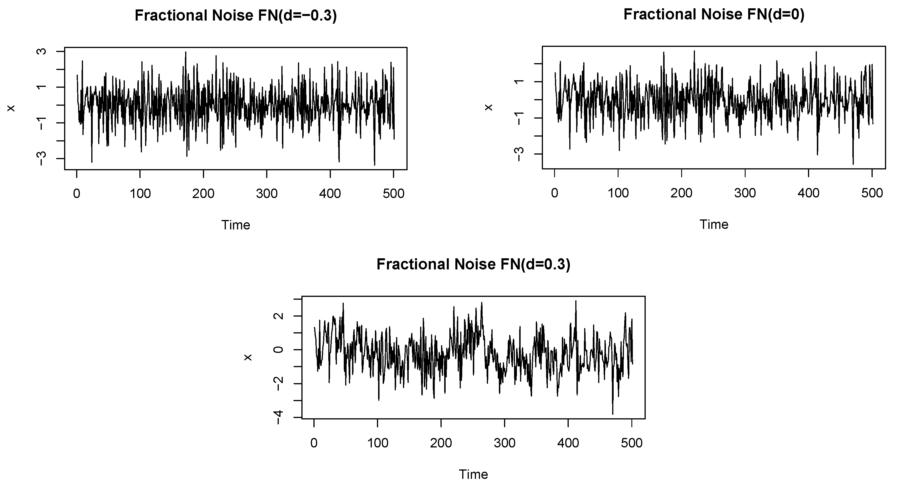
2.1. ARFIMA Model for Long Memory Processes

Autoregressive Fractionally Integrated Moving Average (ARFIMA) models are used to model time series data that exhibit long memory or fractional integration, meaning that the autocorrelation of the series declines very slowly. These models extend the ARIMA models by incorporating a fractional differencing parameter, which allows them to capture the long memory effect. ARFIMA models are particularly useful in modeling and forecasting financial and economic time series with long memory, such as stock prices, exchange rates, and interest rates, and are used in option pricing and volatility forecasting as well. However, estimating these models can be computationally intensive, and interpreting their parameters can be challenging [23].

A stochastic process $\left\{Y_t\right\}$ follows an ARFIMA $(p,d,q)$ process, where p and q are integers and d is a real number, if $\left\{Y_t\right\}$ can be represented as follows:

$$\varphi \left(B\right){(1-B)}^d{Y}_t=\theta \left(B\right){\epsilon }_t,{\epsilon }_t\sim WN(0,{\sigma }_{ϵ}^2),$$

(1)

where $\varphi \left(B\right)=1-{\sum }_{i=1}^p{\varphi }_i{B}^i$ and $\theta \left(B\right)=1+{\sum }_{i=1}^q{\theta }_i{B}^i$ are the polynomials of the autoregressive and moving average operators, respectively. These polynomials do not have roots in common.

The spectral density of the ARFIMA process is provided by

$$f\left(\lambda \right)=|1-e^{i\lambda }{|}^{-2d}\frac{{\sigma }_{ϵ}^2}{2\pi }\frac{|\theta \left(e^{i\lambda }\right){|}^2}{|\varphi \left(e^{i\lambda }\right){|}^2}$$

(2)

where $|1-e^{i\lambda }|=2sin\left(\frac{\lambda }{2}\right)$ and i denotes the imaginary unit. Hosking [24] described the fractionally differentiated process (FN(d)) with polynomials $\varphi \left(B\right)=\theta \left(B\right)=1$ and with the spectral density provided by

$$f\left(\lambda \right)\sim \frac{{\sigma }_{\epsilon }^2}{2\pi }{|1-e^{i\lambda }|}^{-2d}.$$

(3)

Thus, the spectral density has a pole at 0 for $d>0$, leading to $d=H-\frac{1}{2}$, thereby finding the relationship between the fractional differentiation parameter d and the Hurst exponent H.

As demonstrated in Hassani’s ½-theorem, it is important to note that the sum of the sample ACF is always negative one-half for any stationary time series with any length. For this reason, relying solely on the sample ACF to identify long memory processes can be misleading.

2.2. Long Memory Parameter Estimation Methods

2.2.1. Periodogram Regression Method

Under the assumption that the spectral density of a stationary process can be written as

$$f\left(\lambda \right)=f_0\left(\lambda \right){(2sin(\lambda /2))}^{-2d},$$

(4)

where $f_0\left(\lambda \right)=2\pi {\sigma }^{-2}{f}_y\left(\lambda \right){|\lambda |}^{2d}$ is a continuous function with $f_y$ as the strictly positive spectral density of $\left\{y_t\right\}$, Geweke et al. [19] proposed a regression method for estimating the parameters; by defining $y_j=log\left(I\left({\lambda }_j\right)\right)$, $\alpha =log\left(f_0\left(0\right)\right)$, $\beta =-d$, $x_j=log\left({[2sin({\lambda }_j/2)]}^2\right)$, and

$${\epsilon }_j=log\left(\frac{I\left({\lambda }_j\right){[2sin(\lambda /2)]}^{2d}}{f_0\left(0\right)}\right),$$

(5)

the regression equation is obtained as

$$y_j=\alpha +\beta x_j+{\epsilon }_j.$$

(6)

The least squares estimator of the long memory parameter d is provided by

$${\widehat{d}}_m=-\frac{{\sum }_{j=1}^m(x_j-\overline{x})(y_j-\overline{y})}{{\sum }_{j=1}^m{(x_j-\overline{x})}^2},$$

(7)

where $\overline{x}=\frac{1}{m}{\sum }_{j=1}^m{x}_j$ and $\overline{y}=\frac{1}{m}{\sum }_{j=1}^m{y}_j$.

2.2.2. Whittle Estimator Method

Whittle’s estimator [20] is based on the periodogram. This involves the following equation:

$$Q\left(\eta \right)={\int }_{-\pi }^{\pi }\frac{I\left(\lambda \right)}{f(\lambda ,\eta )}d\lambda +{\int }_{-\pi }^{\pi }log\left(f(\lambda ,\eta )\right)d\lambda ,$$

(8)

where $f(\lambda ,\eta )$ is the spectral density at the frequency $\lambda$, $\eta$ is the vectors of the unknown parameters, and $I\left(\lambda \right)$ is the periodogram, defined here as

$$I\left(\lambda \right)=\frac{1}{2\pi n}{\left|\sum _{j=1}^n{Y}_{j}exp\left(ij\lambda \right)\right|}^2.$$

(9)

The second term in Equation (8) can be set to equal to 0 by renormalizing $f(\lambda ,\eta )$. The normalization only depends on a scale parameter, not on the rest of the components of $\eta$; thus, we replace f with $f^{*}$ such that $f^{*}=\beta f$ and ${\int }_{-\pi }^{\pi }log\left(f^{*}(\lambda ,\eta )\right)d\lambda =$0. Because $I\left(\lambda \right)$ is an estimator of the spectral density, a series with long-range dependence should have a periodogram which is proportional to ${|\lambda |}^{1-2H}$ at the origin. Whittle’s estimator is the value of $\eta$ that minimizes the Q function. In actual application, instead of an integral, the corresponding sum over the Fourier frequencies ${\lambda }_j=2\pi j/n$ is computed, where $j=1,2,\dots (n-1)/2$ and n is the length of the series. Thus, the actual function which the algorithm minimizes is

$$\begin{array}{c}\hfill Q^{*}\left(\eta \right)=\sum _{j=1}^{(n-1)/2}\frac{I\left(\lambda \right)}{f^{*}({\lambda }_j,\eta )}.\end{array}$$

(10)

If $\left\{Y_t\right\}$ is fractional Gaussian noise, then $\eta$ is the parameter H or d. If $\left\{Y_t\right\}$ follows an ARFIMA $(p,d,q)$ process, $\eta$ includes the unknown coefficients of the autoregressive and moving average parts of that model. This estimator assumes that the parametric form of the spectral density is known. For more details, see [25].

2.2.3. Detrended Fluctuation Analysis

Detrended fluctuation analysis (DFA) was introduced by Peng et al. [18], and proceeds as follows. Let $\{y_1,y_2,\dots ,y_n\}$ be a sample of a stationary process with a long memory and let $x_t={\sum }_{j=1}^t{y}_j$ for $t=1,\dots ,n$. A sample $\{y_1,y_2,\dots ,y_n\}$ is divided into k blocks without overlap which contain $m=n/k$ observations. A linear regression model of $x_t$ versus t within each block is fitted. Let ${\sigma }_k^2$ be the estimated residual variance of the regression within the block, and let k be the dual variance of the regression within block k:

$${\sigma }_k^2=\frac{1}{m}\sum _{t=1}^m{(x_t-{\widehat{\alpha }}_k-{\widehat{\beta }}_{k}t)}^2$$

(11)

where ${\widehat{\alpha }}_k$ and ${\widehat{\beta }}_k$ are the least squares estimators of the intercept and slope of the regression line, respectively. Furthermore, let $F^2\left(k\right)$ be the average of these variances:

$$F^2\left(k\right)=\frac{1}{k}\sum _{j=1}^k{\sigma }_j^2.$$

(12)

For a random walk, the last term behaves as $F\left(k\right)\sim c{k}^{1/2}$, while for a time series with long dependence we have $F\left(k\right)\sim c{k}^{d+1/2}$. Thus, an estimator of d can be obtained as $\widehat{d}=\widehat{\beta }-1/2$ by applying the least squares estimator to $log\left(F\left(k\right)\right)=\alpha +\beta log\left(k\right)+{\epsilon }_k$.

2.2.4. Rescaled Range Method

Let $\{y_1,y_2,\dots ,y_n\}$ be a sample of a stationary long memory process, let $x_t={\sum }_{j=1}^t{y}_j$ for $t=1,\dots ,n$, and let $s_n^2=\frac{1}{(n-1)}{\sum }_{t=1}^n{(y_t-\overline{y})}^2$ be the sample variance, where $\overline{y}=x_n/n$. The rescaled range statistic introduced by Hurst [16] is defined by

$$R_n=\frac{1}{s_n}\left[\underset{1\le t\le n}{max}\left(x_t-\frac{t}{n}{x}_n\right)-\underset{1\le t\le n}{min}\left(x_t-\frac{t}{n}{x}_n\right)\right].$$

(13)

2.2.5. Wavelet-Based Method

A real-value integrable function $\psi \left(t\right)$ is defined as a wavelet if it satisfies $\int \psi \left(t\right)dt=0$. The family of dilations and translations of the wavelet function $\psi$ is defined by

$${\psi }_{jk}\left(t\right)=2^{-j/2}\psi (2^{-j}t-k),j,k\in \mathbb{Z}.$$

(14)

Here, the terms j and $2^j$ are called the octaves and scale, respectively. With this, we can define the discrete wavelet transform (DWT) of a process $\left\{y\right(t\left)\right\}$ as

$$d_{jk}=\int y\left(t\right){\psi }_{jk}\left(t\right)dt,j,k\in \mathbb{Z}.$$

(15)

Moreover, the family $\left\{{\psi }_{jk}\left(t\right)\right\}$ forms an orthogonal basis, and the representation of the process $\left\{y\right(t\left)\right\}$ is

$$y\left(t\right)=\sum _{j=-\infty }^{\infty }\sum _{k=-\infty }^{\infty }{d}_{jk}{\psi }_{jk}\left(t\right).$$

(16)

Now, we define the statistic

$${\widehat{\mu }}_j=\frac{1}{n_j}\sum _{k=1}^{n_j}{\widehat{d}}_{jk}^2,$$

(17)

where $n_j$ is the number of coefficients in octave j available to be calculated. Veitch et al. [21] demonstrated that

$${\widehat{\mu }}_j\sim \frac{z_j}{n_j}{\chi }_{n_j},$$

(18)

where $z_j=2^{2dj}c$, $c>0$, and ${\chi }_{n_j}$ is a chi-square random variable with $n_j$ degrees of freedom.

The heteroscedastic regression model can be written as

$$y_j=\alpha +\beta x_j+{\epsilon }_j,$$

(19)

where ${\epsilon }_j={log}_2(log\left({\chi }_{n_j}\right))-{log}_2\left(n_j\right)-\psi (n_j/2)+log(n_j/2)$ with $y_j={log}_2\left({\widehat{\mu }}_j\right)-\psi (n_j/2)+log(n_j/2)$, $\alpha =log\left(c\right)$, and $\beta =2d$. Therefore, when the estimator $\widehat{\beta }$ is obtained, an estimate for the long memory parameter d is provided by $\widehat{d}=\widehat{\beta }/2$. Furthermore, it follows that $Var\left(\widehat{d}\right)=Var\left(\widehat{\beta }\right)/4$.

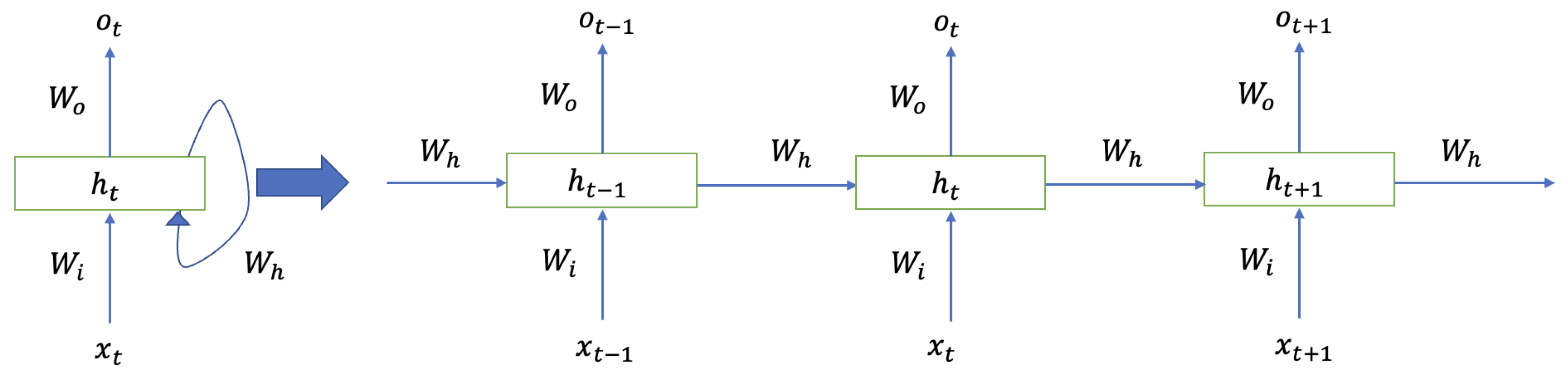
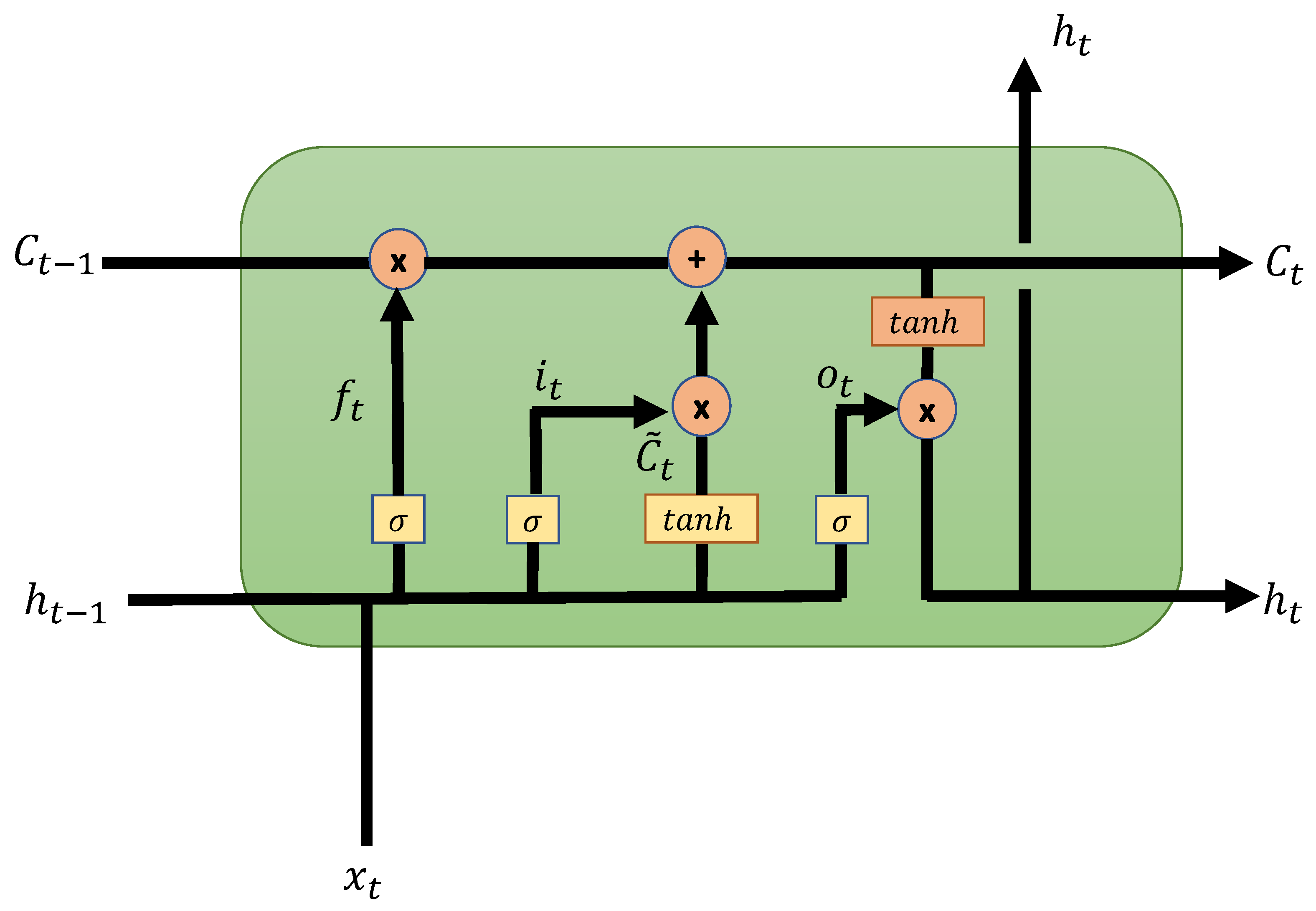
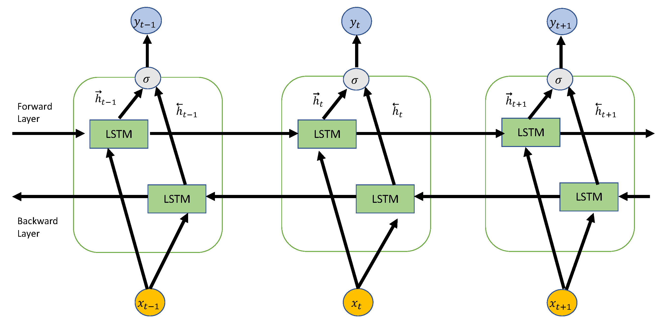
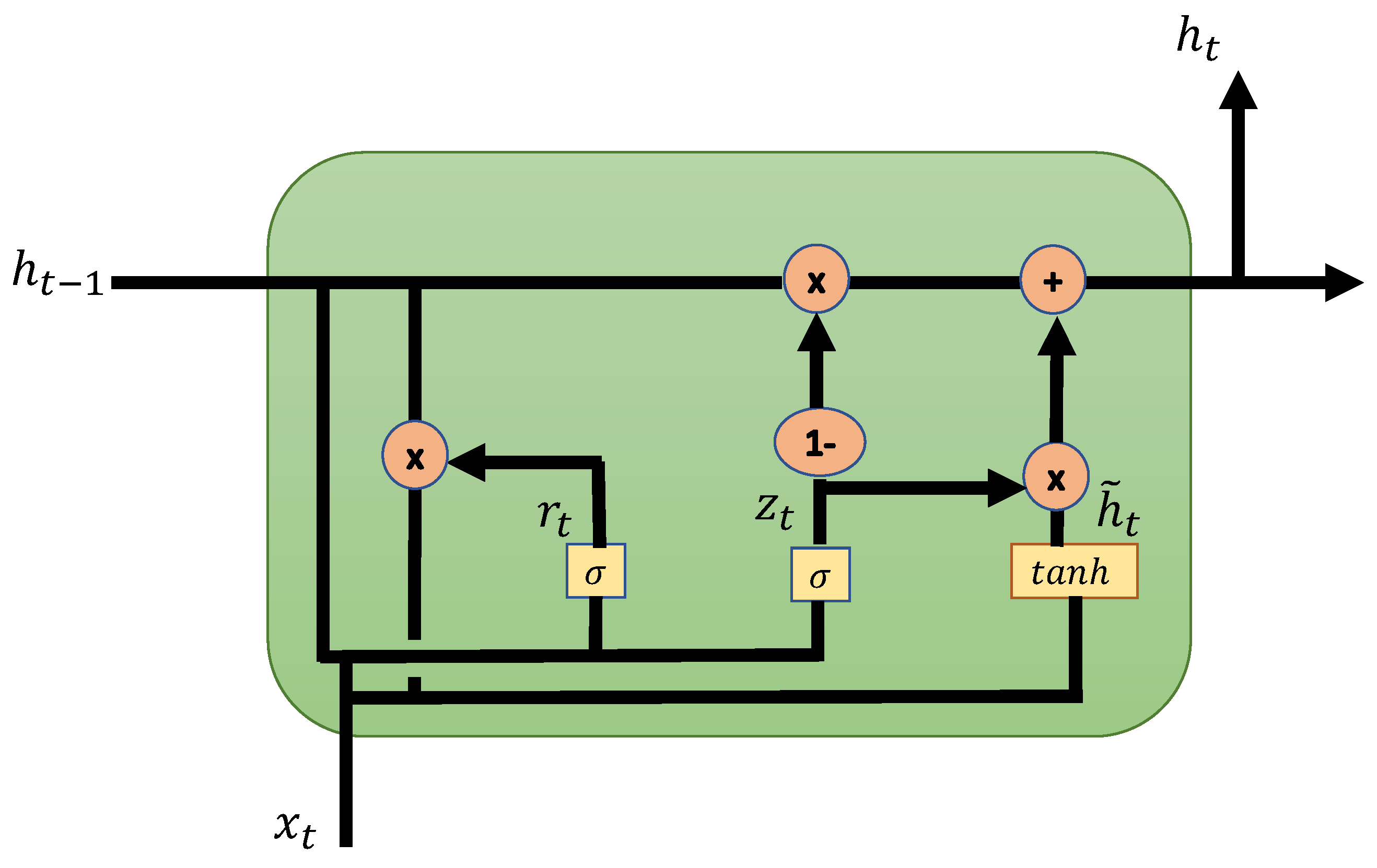
2.3. Recurrent Artificial Neural Networks

Artificial Neural Network (ANN) models consist of layers of nonlinear processing units called neurons that are linked to each other by weighted connections. These models use the backpropagation algorithm to learn from data by fitting the weights of the connections between the neurons [26]. ANNs are highly parameterized nonlinear models capable of learning from data. Moreover, they are universal function approximations that learn from data (see Cybenko [27] and Hornik et al. [28]), and have been successfully applied in time series forecasting (for instance, see [2]). Specifically, ANN models outperform standard linear techniques when the time series is noisy and the underlying dynamical system is nonlinear [12].

Deep Recurrent Neural Networks (RNN) are a subclass of Artificial Neural Networks (ANN) in which the processing units, or neurons, may be grouped either in layers or blocks connected to the following units (feedforward connections) or to previous units (feedback or recurrent connections). These feedback connections introduce memory to the model structure. By using these recurrent connections, historical inputs can be “memorized” by the RNN and subsequently influence the network’s output. The “memory” that RNNs possess allows them to outperform feedforward neural networks (FNN) in many real-world applications.

Recurrent Neural Networks (RNN) are ANNs with at least one recurrent connection, and are capable of learning features and long-term dependencies from sequential and time series data [29]. Moreover, RNNs are universal approximations [30]. Hochreiter [31] introduced the Long Short-Term Memory Network (LSTM), an RNN consisting of memory cells and gate units. LSTMs address the vanishing gradient problem [32,33]. LSTMs can learn long-term dependencies, and are well known for working with sequential data. Later, Graves et al. [34] proposed the Bidirectional LSTM (BiLSTM) network, which consists of two LSTMs, the first taking the input in a forward direction and the second in a backward direction. Cho et al. [35] proposed a simplified version of the LSTM called Gated Recurrent Unit (GRU), which lacks an output gate.

Figure 1 shows the structure of a simple RNN [36], where $x_t$ is the mini-batch input of the t-th time step in the sequence and $h_t=f_{\sigma }(W_i{x}_t+W_i{h}_{t-1}+b_r)$ is the hidden variable of the time step t, which is determined by both the input of the current time step and the hidden variable of the previous time step. The RNN stores the hidden variable $h_{t-1}$ for the previous time step and introduces a new weight parameter $W_h$ to describe how the hidden variable of the previous time step is used for the current time step. An RNN can be understand as multiple replications of the same network; during each replication, a state is transferred to the next layer, and the hidden variables can be used to capture the historical information of the sequence up to the current time step. This means that the neural network is able to memorize information. The calculation formula for the output layer is as follows:

$$o_t=f_{\sigma }(W_o{h}_t+W_i+b_o).$$

(20)

The parameters of the RNN include the hidden layer weights $W_i$ and $W_h$, the hidden layer bias $b_r$, the output layer weight $W_o$, and the output layer bias $b_o$.

A Long Short-Term Neural Network (LSTM) is a variant of the Recurrent Neural Network (RNN) proposed by Hochreiter et al. [31]. An LSTM has a similar basic structure to an RNN, except that memory blocks replace neurons. Each memory block contains three nonlinear units called gates. The input gate $i_t$, the output gate $o_t$, and the forget gate $f_t$ control the information in the network. The memory of the cell is controlled by the hidden state $h_t$ and the cell state $c_t$. Figure 2 shows the diagram of the LSTM block.

At the time t, the input vector $x_t\in {\mathbb{R}}^d$ flows forward in the LSTM cell, where the operations formula are:

$$\begin{array}{ccc}\hfill \mathrm{Input} \mathrm{Gate}:& i_t=& f_{\sigma }(W_i{x}_t+U_i{h}_{t-1}+b_i)\hfill \end{array}$$

(21)

$$\begin{array}{ccc}\hfill \mathrm{Forget} \mathrm{Gate}:& f_t=& f_{\sigma }(W_f{x}_t+U_f{h}_{t-1}+b_f)\hfill \end{array}$$

(22)

$$\begin{array}{ccc}\hfill \mathrm{Output} \mathrm{Gate}:& o_t=& f_{\sigma }(W_o{x}_t+U_o{h}_{t-1}+b_o)\hfill \end{array}$$

(23)

$$\begin{array}{ccc}\hfill \mathrm{Hidden} \mathrm{State}:& h_t=& o_t\odot tanh\left(c_t\right)\hfill \end{array}$$

(24)

$$\begin{array}{ccc}\hfill \mathrm{Cell} \mathrm{State}:& c_t=& f_t\odot c_{t-1}+i_t\odot tanh(W_c{x}_t+U_c{h}_{t-1}+b_c)\hfill \end{array}$$

(25)

where $W_i$, $W_f$, $W_o$, $W_c$$U_i$, $U_f$, $U_o$, $U_c$ correspond to the weight matrices and $b_i$, $b_f$, $b_o$, $b_c$ are the bias vectors. The initial values are $c_0=0$ and $h_0=0$. The activation functions are the sigmoid function $f_{\sigma }\left(z\right)=\frac{1}{1+e^{-z}}$ and the hyperbolic tangent function $tanh\left(z\right)=\frac{e^z-e^{-z}}{e^z+e^{-z}}$. The operator ⊙ denotes the Hadamard product.

The Bidirectional LSTM Network (BiLSTM) proposed by Graves et al. [34] is a sequence processing model that consists of an LSTM with two hidden states that allows the information to flow both forward and backward. Figure 3 shows the architecture of the BiLSTM. After processing each time step t, the BiLSTM network generates two hidden states $h_t^F$ and $h_t^B$.

A Gated Recurrent Unit (GRU) is a simpler version of the LSTM network proposed by Cho et al. [35]. Figure 4 shows the architecture of the GRU. The input vector $x_t$ is introduced to the network, passing through both the update gate $z_t$ and the reset gate $z_t$. On the one hand, the update gate decides how the input $x_t$ and the previous output $h_t$ flow to the next cell. On the other hand, the reset gate determines how much past information can be forgotten. The equations that control the functionality of the GRU are:

$$\begin{array}{ccc}\hfill \mathrm{Update} \mathrm{Gate}:& z_t=& f_{\sigma }(W_z{x}_t+U_z{h}_{t-1}+b_z)\hfill \end{array}$$

(26)

$$\begin{array}{ccc}\hfill \mathrm{Reset}\mathrm{Gate}:& r_t=& f_{\sigma }(W_r{x}_t+U_r{h}_{t-1}+b_r)\hfill \end{array}$$

(27)

$$\begin{array}{ccc}\hfill \mathrm{Hidden}\mathrm{State}:& {\tilde{h}}_t=& tanh(W_h{x}_t+U_h(r_t\odot h_{t-1})+b_h)\hfill \end{array}$$

(28)

$$\begin{array}{ccc}\hfill \mathrm{Output}\mathrm{state}:& h_t=& (1-z_t)\odot h_{t-1}+z_t\odot {\tilde{h}}_t\hfill \end{array}$$

(29)

where $W_z$, $W_r$, $W_h$, $U_z$, $U_r$, $U_h$ correspond to the weight matrices and $b_z$, $b_r$, $b_h$, are the bias vectors.

3. Materials and Methods

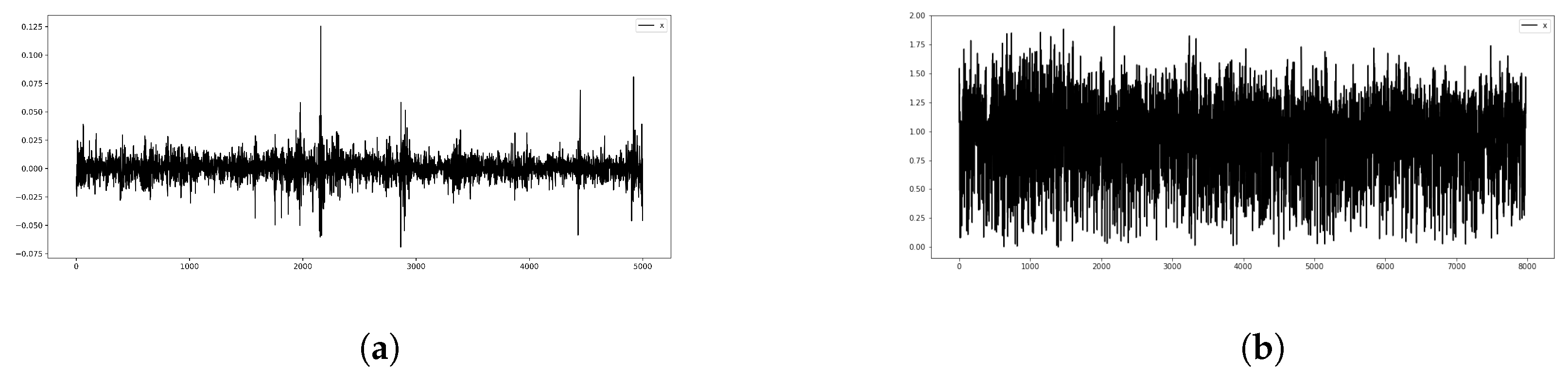
3.1. Dataset Description

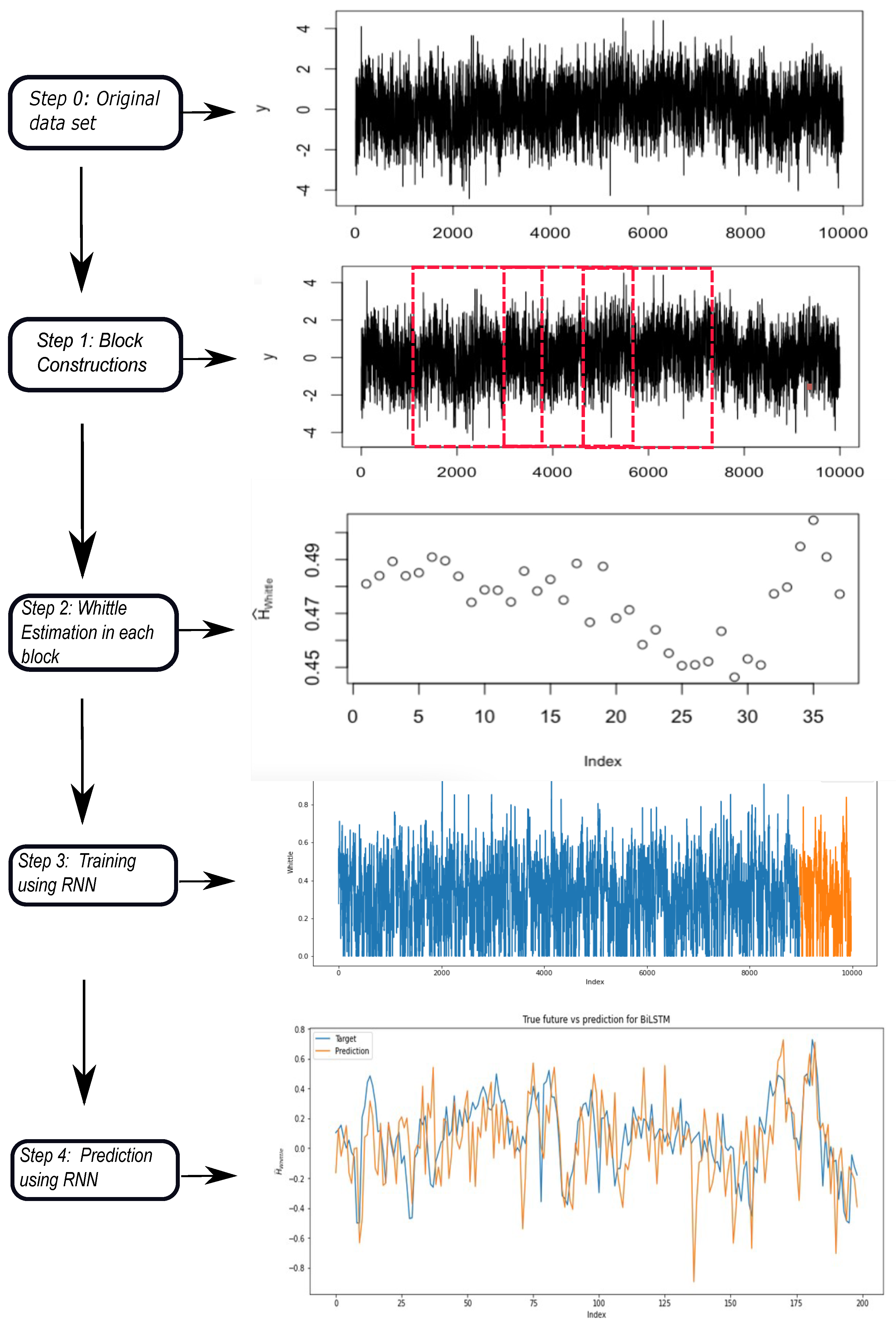
The synthetic data considered in this work for training the networks were artificially constructed and of size $n=\mathrm{10,000}$, which can be seen in Figure 5. These data consisted of fractional noise (FN) obtained with different fractional differentiation parameters d.

The real data that were used to train the networks consisted of: (1) a percentage variation of the IPSA (used in the Santiago Stock Exchange as the primary utility index to measure the profitability of the leading forty stocks that are moving in the economy; these incorporate all the capital changes of each share, weighting the relative weight of each for the calculation) in the period 2000–2021, as can be seen in Figure 6a; and (2) tree-ring widths in dimensionless units recorded by Donald A. Graybill, 1980, from Gt Basin Bristlecone Pine 2805M, 3726-11810 in Methuselah Walk, California, as plotted in Figure 6b. In particular, this time series has been analyzed in several studies, for example in [37].

3.2. Methodology

The purpose of this work is to propose an automated methodology that combines the estimation methodologies of the fractional differentiation parameter (and/or Hurst parameter) with its application to recurrent neural networks such that the network learns and predicts long memory information dependencies obtained in nonlinear time series. The information that is entered in the RNN is obtained from the previously estimated parameter using the Whittle method (chosen from among other estimation methods from a previous study) given data windows of optimal size.

The proposal combines three methods that allow for better approximation in the prediction of the values of the parameters for each one of the windows obtained. The proposed approach makes predictions of the Hurst exponent values by learning the estimate obtained using conventional methods applied to a moving time window.

The scheme of this methodology is shown in Figure 7.

The proposed methodology consists of three main steps. The first step is to divide the sample $\{Y_1,\dots ,Y_T\}$ into a number M of overlapping blocks of length N and with a shift of S such that $T=S(M-1)+N$ and the midpoint of the j-th block is obtained as $t_j=S(j-1)+N/2$ with $j=1,\dots ,M$. When the data blocks are determined, the second step of the methodology consists of obtaining the Hurst exponent’s local estimates over each block using the Whittle estimation method. The idea of segmenting the time series is provided by Palma et al. [38], among others. The methodology for approximating the MLE is based on the calculation of the periodogram $I\left(\lambda \right)$ by means of the fast Fourier transform (FFT), e.g., [39], and the use of the approximation of the Gaussian log-likelihood function follows Whittle [40] and Bisaglia [41]. Suppose that the sample vector $Y=(y_1,y_2,\dots ,y_n)$ is normally distributed with zero mean and with the autocovariance provided by

$$\gamma (k-j)={\int }_{-\pi }^{\pi }f\left(\lambda \right)e^{i\lambda (k-j)}d\lambda ,$$

(30)

where $f\left(\lambda \right)$ is defined as in (2) and is associated with the parameter set $\mathrm{\Theta }$ of the ARFIMA model defined in (1). The log-likelihood function of the process Y is provided by

$$\mathcal{L}\left(\mathrm{\Theta }\right)=-\frac{1}{2n}[log|\mathrm{\Delta }|-Y^T{\mathrm{\Delta }}^{-1}Y],$$

(31)

where $\mathrm{\Delta }=\left[\gamma \right(k-j\left)\right]$ with $k,j=1,\dots ,n$. For calculating (31), two asymptotic approximations are made for the terms $log(|\mathrm{\Delta }|)$ and $Y^T{\mathrm{\Delta }}^{-1}Y$ to obtain

$$\mathcal{L}\left(\mathrm{\Theta }\right)\approx -\frac{1}{4\pi }\left\{{\int }_{-\pi }^{\pi }log\left[2\pi f\left(\lambda \right)\right]d\lambda +{\int }_{-\pi }^{\pi }\frac{I\left(\lambda \right)}{f\left(\lambda \right)}d\lambda \right\},$$

(32)

as $n\to \infty$ where $I\left(\lambda \right)=|{\sum }_{j=1}^n{y}_j{e}^{i\lambda j}{|}^2/\left(2\pi n\right)$ is the periodogram indicated before. Thus, a discrete version of (32) is the Riemann approximation of the integral, and is

$$\mathcal{L}\left(\mathrm{\Theta }\right)\approx -\frac{1}{2n}\left\{\sum _{j=1}^{n}log\left[f\left({\lambda }_j\right)\right]+\sum _{j=1}^n\frac{I\left({\lambda }_j\right)}{f\left({\lambda }_j\right)}\right\},$$

(33)

where ${\lambda }_j=2\pi j/n$ are the Fourier frequencies. Now, to find the estimator of the parameter vector $\mathrm{\Theta }$, we use the minimization of ${\mathcal{L}}_T\left(\mathrm{\Theta }\right)$ produced by the relation

$$\widehat{\mathrm{\Theta }}=arg\; min\mathcal{L}\left(\mathrm{\Theta }\right),$$

(34)

where the minimization is over a parameter space $\mathrm{\Theta }$. This nonlinear minimization function carries out a minimization of $\mathcal{L}\left(\mathrm{\Theta }\right)$ using a Newton-type algorithm. Under regularity conditions, the Whittle estimator that maximizes the log-likelihood function provided in (33) is consistent and distributed normally (e.g., [42]). This estimation method has been used in studies on local seasonal series (see [43,44]), and the use of this estimator in this work is justified later on in the subsequent comparative study.

The time series is separated into two segments, where the first partition, corresponding to 90% of the samples, is used for training and the final segment, corresponding to 10% of the samples, is used for testing. The recurrent neural networks are fitted with the training set, then the models are compared and validated on the test set. The RNNs are explained in the following subsection.

In order to obtain the predictions and measure their performance, we use measures such as the Root Mean Square Error (RMSE) and Coefficient of Determination $R^2$.

The RMSE is often preferred over the MSE, as it is on the same scale as the data. Historically, both the RMSE and MSE have seen widespread use due to their theoretical relevance in statistical modeling. However, they are more sensitive to outliers than the MAE, which has led a number of authors, e.g., [45], to recommend their use in assessing forecasting accuracy.

A two-sample two-sided Kolmogorov–Smirnov (KSPA) test, as proposed by Hassani et al. [15], was applied to determine the existence (or not) of statistical significant differences in the distribution of forecasts between the two models with the best performances.

The pseudo-code of the proposed methodology is provided in Algorithm 1.

Algorithm 1 Predicting the Hurst parameter

1: Define the block length N and the shift S. 2: Segment the blocks of size N from the Times Series. 3: for each block $j=1$ to M do 4:     Apply the Whittle method given by Equation (33) to obtain the value of the Hurst Exponent at time $t_j=S(j-1)+N/2$. 5: end for 6: Separate the blocks of the original Time Series into training and test sets. 7: Separate the Hurst’s Time Series into training and test sets. 8: Fit the RNN (simpleRNN, LSTM, BiLSTM or GRU) using the training sets. The inputs are the blocks of the original Time series and the targets are the Hurst’s time series. 9: for each block in the Test set do 10:     Predict the value of the Hurst parameter for the next block using the RNN. 11: end for 12: Obtain the performance metrics for the test set: Root Mean Square Error (RMSE) and the Coefficient of Determination $R^2$.

4. Results

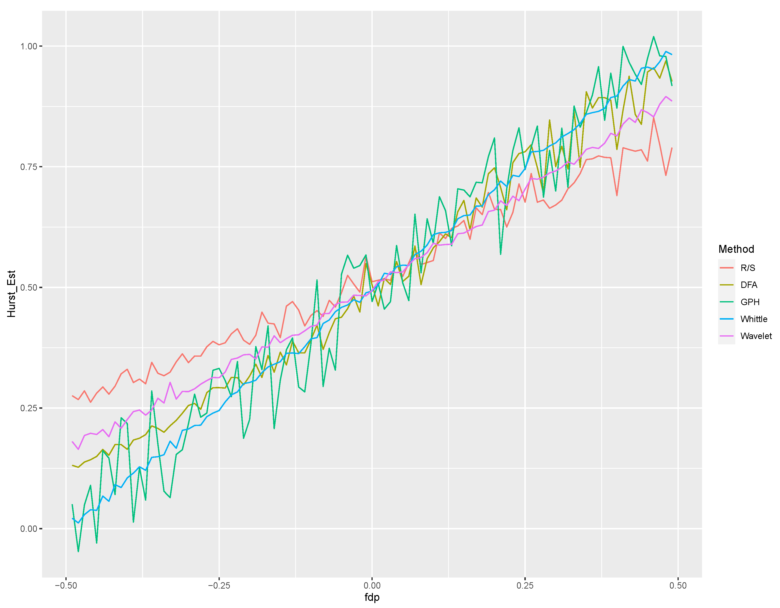
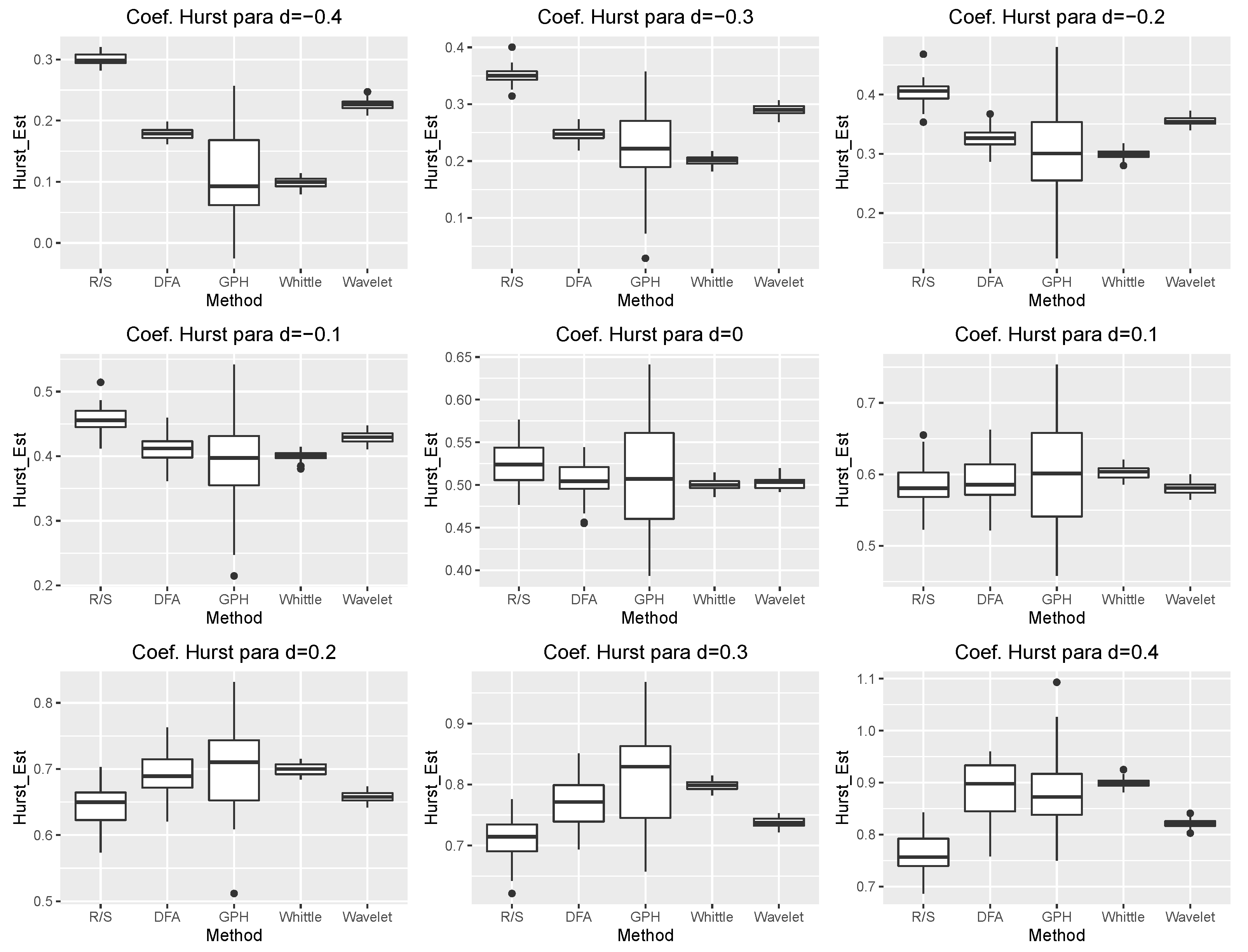
4.1. Comparative Study of Estimation Methods

In this section, a comparative study of the following estimation methods is carried out: the periodogram regression method, Whittle estimator method, detrended fluctuation analysis, rescaled range method, and wavelet-based method. In addition, a Monte Carlo simulation was performed using simulated time series of sizes $n=\mathrm{10,000}$ with specific values of the fractional differentiation parameter and 1000 simulations.

Figure 8 and Figure 9 show the degree of fit of the different estimation methods with the Hurst parameter and the fractional differentiation parameter.

From Figure 8, it can be seen that with $n=\mathrm{10,000}$, the estimation methods of the Hurst exponent concerning the differentiation parameter d stabilize around the relationship obtained in the ARFIMA(d), as provided by $H=d+0.5$. It can be observed that at around $d=-0.5$ ($H=0$) the Whittle method fits better than the rest of the methods, which either deviate from the true value or have unstable behavior, such as in the GPH method. Around $d=0$ ($H=0.5$), all of the models fit the relationship between said parameters well except for the GPH method. Finally, around $d=0.5$ ($H=1$) the behavior of the methods becomes unstable except in the case of the Whittle method. From this, it can be concluded that Whittle’s method is the one that best fits this relationship in the interval of a good definition of the fractional differentiation parameter. This behavior occurs in the Whittle and wavelet-based methods, as they are better able to fit the relationship, as shown by Figure 9 for all the values of the fractional differential parameter. These methods show less dispersion in the Hurst parameter estimates; however, the Whittle method shows more stability, while the GPH method shows a greater range of dispersion in its estimates. In particular, little dispersion is observed in almost all methods except the GPH method when $d<0$, although they are claimed from the objective value. When d approaches 0, the R/S and DFA methods increase their dispersion even though it approach the target value, as the R/S, DFA, and GPH methods are already unstable in their dispersion when $d>0$. We use the Whittle method in what follows based on the previous results, which are consistent with those obtained by Palma et al. [38].

4.2. Hurst Parameter Prediction Using Recurrent Neural Networks

4.2.1. Synthetic Data

Table 1. Performance results and training time for prediction of the Hurst parameter for the $FN(d=-0.3)$ simulated data using recurrent neural networks.

		d $=-0.3$
		${\mathit{R}}^{\mathbf{2}}$				RMSE				Training Time (s)
		sRNN	BiLSTM	LSTM	GRU	sRNN	BiLSTM	LSTM	GRU	sRNN	BiLSTM	LSTM	GRU
S = 1	18	0.721	0.742	0.706	0.729	0.171	0.164	0.175	0.168	130.9	262.3	220.9	258.7
	20	0.709	0.746	0.716	0.736	0.161	0.151	0.160	0.154	104.5	233.4	207.0	255.1
	23	0.673	0.724	0.686	0.706	0.150	0.138	0.148	0.143	127.2	261.7	235.8	270.2
	25	0.657	0.723	0.676	0.699	0.146	0.131	0.142	0.137	128.6	266.3	265.6	265.4
	28	0.652	0.731	0.666	0.699	0.141	0.125	0.138	0.132	115.1	226.8	215.7	231.1
	30	0.641	0.730	0.646	0.685	0.141	0.122	0.140	0.132	134.5	284.0	226.4	271.5
	33	0.601	0.690	0.616	0.650	0.136	0.120	0.133	0.127	124.0	240.9	209.8	246.3
	35	0.534	0.670	0.605	0.644	0.138	0.116	0.127	0.121	127.1	252.0	213.6	260.2
S = 5	20	0.298	−0.117	0.519	0.532	0.248	0.314	0.206	0.203	34.4	70.4	62.4	79.1
	25	0.282	−0.396	0.440	0.507	0.206	0.290	0.184	0.173	36.9	70.2	69.1	69.5
	30	0.049	−0.217	0.436	0.461	0.234	0.264	0.180	0.176	32.9	76.2	60.4	69.3

,

Table 2. Performance results and training time for prediction of the Hurst parameter for the $FN(d=0)$ simulated data using recurrent neural networks.

		d = 0
		${\mathit{R}}^{\mathbf{2}}$				RMSE				Training Time (s)
		sRNN	BiLSTM	LSTM	GRU	sRNN	BiLSTM	LSTM	GRU	sRNN	BiLSTM	LSTM	GRU
S = 1	18	0.771	0.833	0.776	0.782	0.167	0.142	0.166	0.163	119.0	271.3	228.0	288.6
	20	0.767	0.813	0.761	0.779	0.158	0.141	0.159	0.154	116.2	220.5	209.8	241.7
	23	0.730	0.807	0.721	0.754	0.144	0.122	0.147	0.138	122.8	226.1	190.7	237.7
	25	0.713	0.800	0.700	0.747	0.142	0.118	0.145	0.133	168.5	329.7	303.2	344.3
	28	0.721	0.815	0.697	0.737	0.132	0.108	0.138	0.128	144.3	316.6	264.3	298.5
	30	0.686	0.812	0.672	0.720	0.124	0.104	0.137	0.127	113.3	214.8	197.0	232.3
	33	0.654	0.781	0.650	0.689	0.125	0.099	0.126	0.118	119.9	212.5	188.4	221.3
	35	0.670	0.782	0.611	0.673	0.114	0.093	0.124	0.114	131.6	213.0	183.4	216.8
S = 5	20	0.354	0.100	0.516	0.533	0.260	0.306	0.225	0.221	26.5	64.0	43.4	49.2
	25	0.321	−0.060	0.481	0.497	0.215	0.269	0.188	0.186	32.4	51.4	42.5	49.0
	30	0.128	0.125	0.499	0.526	0.232	0.233	0.176	0.171	31.9	52.7	44.0	61.6

and

Table 3. Performance results and training time for prediction of the Hurst parameter for the $FN(d=0.3)$ simulated data using recurrent neural networks.

		d = 0.3
		${\mathit{R}}^{\mathbf{2}}$				RMSE				Training Time (s)
		sRNN	BiLSTM	LSTM	GRU	sRNN	BiLSTM	LSTM	GRU	sRNN	BiLSTM	LSTM	GRU
S = 1	18	0.814	0.852	0.801	0.801	0.155	0.138	0.160	0.160	128.3	293.8	237.6	278.0
	20	0.769	0.860	0.791	0.804	0.157	0.123	0.150	0.145	100.8	221.7	173.6	202.0
	23	0.748	0.869	0.759	0.778	0.142	0.102	0.139	0.133	124.1	239.5	208.3	261.8
	25	0.756	0.877	0.753	0.773	0.135	0.096	0.135	0.130	125.2	249.9	200.1	240.1
	28	0.748	0.882	0.744	0.768	0.129	0.088	0.131	0.124	129.2	281.7	245.7	273.4
	30	0.716	0.884	0.721	0.751	0.129	0.083	0.128	0.121	120.7	260.9	197.2	247.7
	33	0.685	0.859	0.676	0.714	0.121	0.081	0.122	0.115	117.6	229.1	193.3	230.4
	35	0.681	0.845	0.654	0.680	0.114	0.079	0.119	0.114	124.0	223.2	203.8	243.2
S = 5	20	0.375	0.173	0.485	0.518	0.254	0.292	0.230	0.223	37.2	83.0	81.4	82.5
	25	0.368	0.230	0.475	0.479	0.212	0.234	0.193	0.192	39.7	86.7	75.3	104.2
	30	0.307	0.111	0.461	0.504	0.208	0.235	0.183	0.176	38.9	84.1	83.5	85.9

show the performance results of these models. We ran ten simulations for each model, then the results were averaged, which are the results appearing in the tables below. It can be seen that the performance metrics for the test set are better on the BiLSTM network. For the best two models, we applied the Shapiro–Wilk test to check the normal distribution of the performances and the pooled variance t-test to verify statistical differences. Moreover, the KSPA test was applied to verify the statistical significance of the observed difference in performance.

For $d=-0.3$ and $d=0$, the best results of the coefficient of determination $R^2$ were obtained for small window sizes, specifically, for $N=20$ and $N=18$, respectively. For $d=0.3$, the best result was obtained for $N=30$. In addition, it can be observed that the MAE and RMSE coefficients decrease as block size increases. As the value of the fractional differentiation parameter, and consequently the Hurst exponent, increases within the interval $[-0.5;0.5]$, the value of $R^2$ improves, which indicates that a better prediction is obtained for non-negative values of that parameter.

The same conclusion can be drawn concerning the MAE and RMSE performance indicators, which decrease as the interval mentioned above progresses. Finally, it can be observed that the values of all the indicators are significantly worse for $S=5$, and even yield results with little statistical meaning; thus, in this study, when using real data $S=1$ is considered for the analysis. Regarding the training time of the neural networks, the results of which can be seen in the tables, it can be seen that the BiLSTM network takes the longest for all window sizes, which is clearly due to its architecture. However, this effectively increases the amount of information available to the network, improving its coefficient of determination.

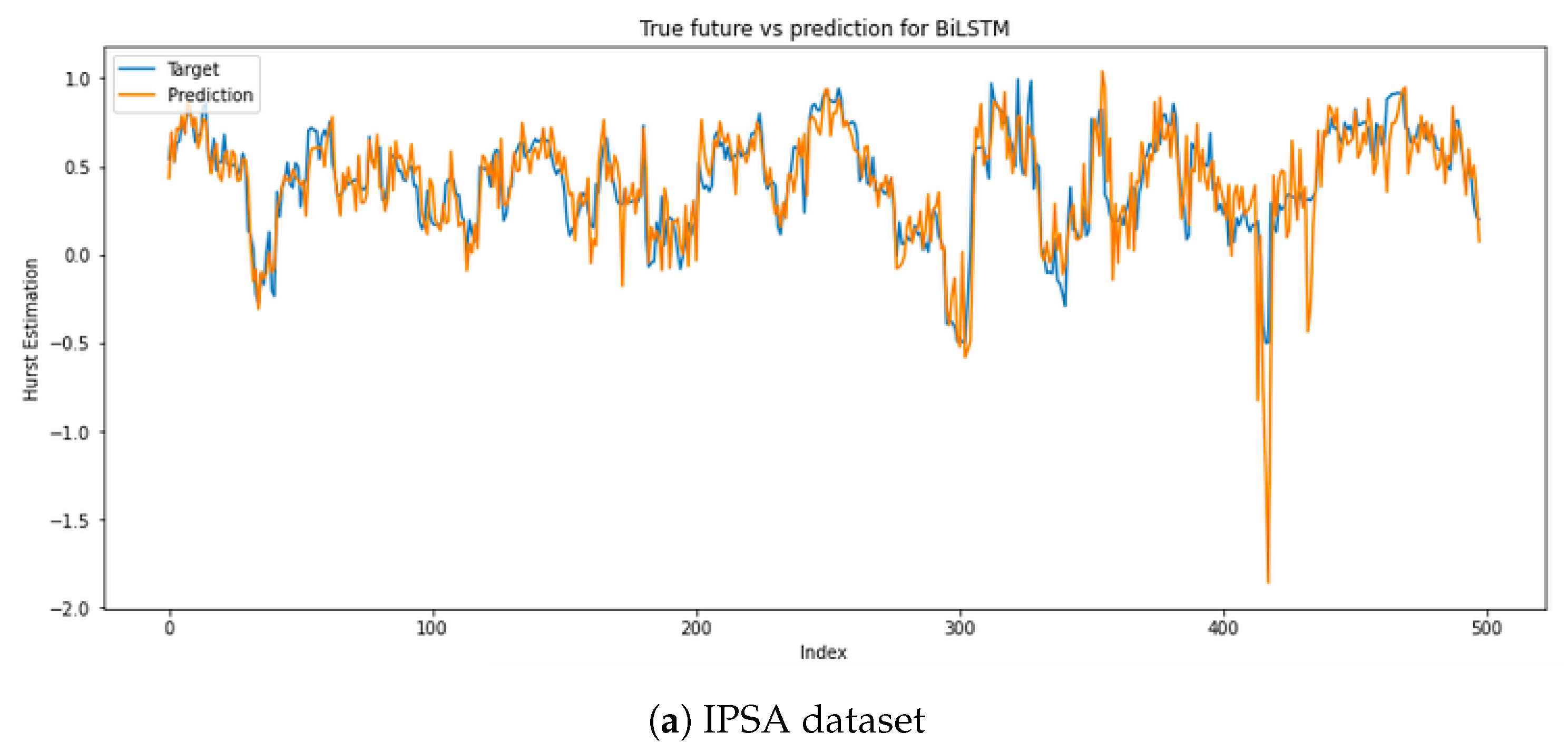
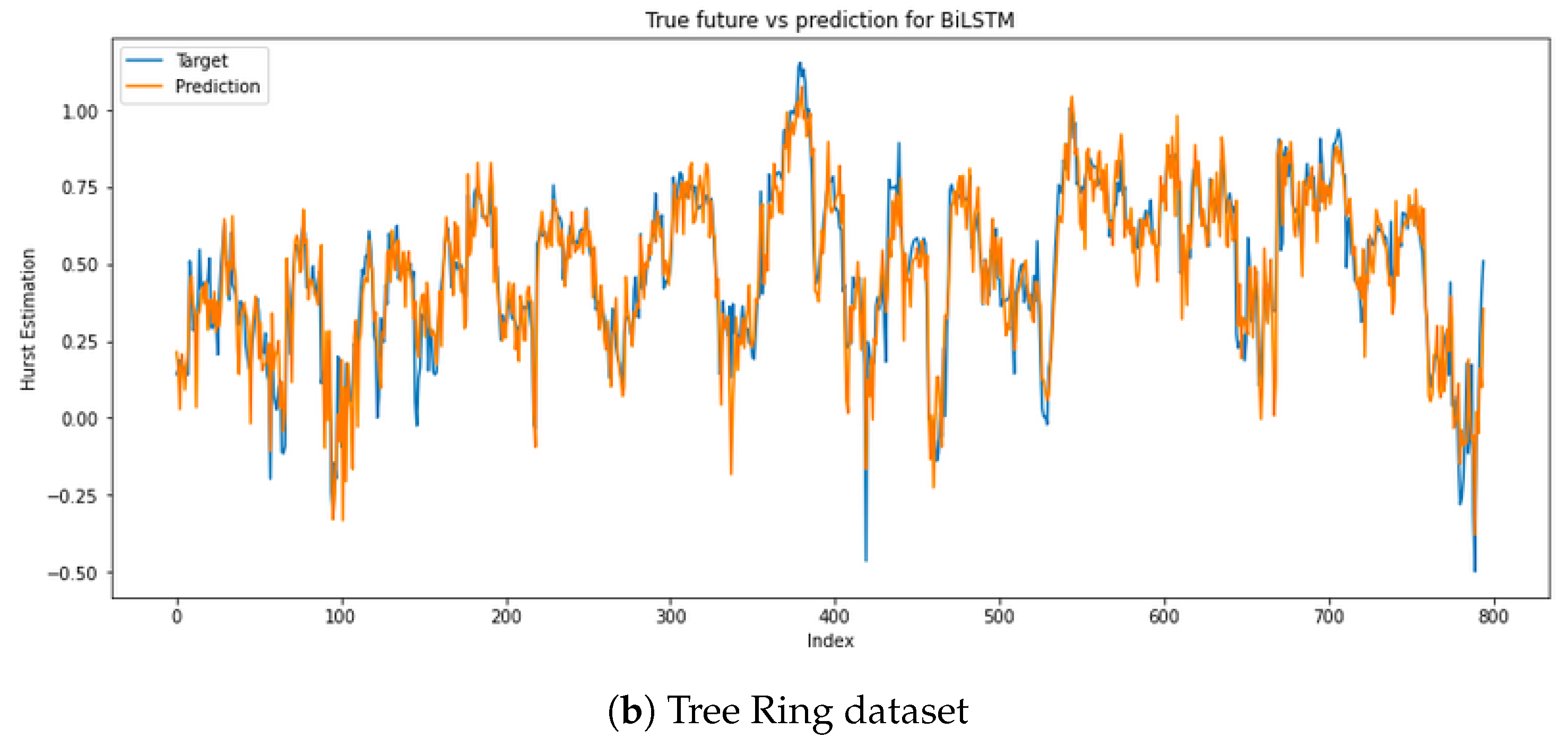
4.2.2. Real Datasets

From the results of the fractional-noise synthetic data in the previous section, the BiLSTM neural network was used for the real dataset using different window sizes $S=1$. As in the case of the synthetic data, we ran ten simulations for each model and the results were averaged, which are the results appearing in the tables below. From

Table 4. Performance results for prediction of the Hurst parameter for the IPSA time series dataset using the BiLSTM Network.

	IPSA Dataset (BiLSTM)
	Train			Test
N	${\mathit{R}}^{\mathbf{2}}$	MAE	RMSE	${\mathit{R}}^{\mathbf{2}}$	MAE	RMSE	Training Time (s)
18	0.912	0.072	0.097	0.679	0.133	0.184	147.659
20	0.922	0.062	0.083	0.716	0.115	0.153	136.575
23	0.936	0.048	0.064	0.651	0.106	0.145	111.459
25	0.938	0.044	0.058	0.621	0.105	0.140	131.349
28	0.944	0.038	0.050	0.437	0.106	0.148	122.480
30	0.948	0.034	0.045	0.396	0.103	0.141	112.823
33	0.952	0.029	0.039	0.398	0.099	0.133	133.320
35	0.955	0.027	0.036	0.348	0.098	0.132	109.261

and

Table 5. Performance results for prediction of the Hurst parameter for the Tree Ring time series dataset using the BiLSTM Network.

	Tree Ring Dataset (BiLSTM)
	Train			Test
N	${\mathit{R}}^{\mathbf{2}}$	MAE	RMSE	${\mathit{R}}^{\mathbf{2}}$	MAE	RMSE	Training (s)
18	0.912	0.076	0.102	0.799	0.109	0.150	169.029
20	0.925	0.066	0.087	0.818	0.097	0.133	149.533
23	0.937	0.052	0.068	0.822	0.084	0.115	251.819
25	0.943	0.046	0.061	0.830	0.080	0.106	259.888
28	0.949	0.042	0.054	0.828	0.074	0.098	259.807
30	0.949	0.039	0.051	0.819	0.073	0.095	224.713
33	0.953	0.035	0.045	0.790	0.071	0.094	247.332
35	0.956	0.032	0.042	0.786	0.069	0.090	245.959

, it can be observed that for the IPSA dataset, the best indices with $N=20$ were obtained in the determination coefficient $R^2$, while for the Tree Ring dataset the best results in the determination coefficient were obtained when $N=25$. It can observed that the MAE and RMSE coefficients both decrease as the size of the window increases. Figure 10 shows the prediction of the values of the Hurst exponent for the real data, reinforcing what was observed in the previous tables. Furthermore, in the last column of Table 4 and Table 5 it can be seen that the training time of the BiLSTM network depends on the size of the dataset and the assigned size of the window N.

Table 6. KS test for prediction of the real time series using the BILSTM Network.

		KS Test
Data	N Opt	Statistic Value	p-Value
IPSA	20	0.0663	0.2244
Treering	25	0.0289	0.8937

indicates that, through the Kolmogorov-Smirnov test, the predictions obtained by the BILSTM network fit the test set of the real data time series. The idea of carrying out this test to check the goodness of fit of the predictions was based, among other studies, on [15].

5. Conclusions

In this work, we have presented a new approach for predicting the Hurst exponent using recurrent neural networks. By applying Whittle’s method using a sliding time window, a new time series corresponding to the estimation of long memory is constructed. Different recurrent neural network models were trained which received data blocks from the original time series as input and generated one-step-ahead predictions of the long memory parameter as output. Our results show that it is possible to have good predictions one step ahead of the long memory parameter; in particular, the BiLSTM network obtained the best results when using the proposed methodology. Additionally, these predictions can be made in real time due to the computational speed of the neural network models.

Further work could include a new procedure that incorporates more complex models with a long memory, and could even involve heteroscedastic behaviors. One of the limitations of our proposed method is that it relies on a fixed size block length, meaning that the RNN cannot successfully capture points located very distant from the signal. Further work is required to enhance prediction when the size of the overlapping blocks changes dynamically, together with a rehearsal mechanism for incremental learning. In our future work, we expect to correlate the temporal estimation of long-term memory in order to improve prediction of the volatility of GARCH models.

References

1. Di Giorgi, G.; Salas, R.; Avaria, R.; Ubal, C.; Rosas, H.; Torres, R. Volatility Forecasting using Deep Recurrent Neural Networks as GARCH models. Comput. Stat. 2023, 1–27. [Google Scholar] [CrossRef]
2. Cordova, C.H.; Portocarrero, M.N.L.; Salas, R.; Torres, R.; Rodrigues, P.C.; López-Gonzales, J.L. Air quality assessment and pollution forecasting using artificial neural networks in Metropolitan Lima-Peru. Sci. Rep. 2021, 11, 24232. [Google Scholar] [CrossRef]
3. Leite Coelho da Silva, F.; da Costa, K.; Canas Rodrigues, P.; Salas, R.; López-Gonzales, J.L. Statistical and artificial neural networks models for electricity consumption forecasting in the Brazilian industrial sector. Energies 2022, 15, 588. [Google Scholar] [CrossRef]
4. Vivas, E.; de Guenni, L.B.; Allende-Cid, H.; Salas, R. Deep Lagged-Wavelet for monthly rainfall forecasting in a tropical region. Stoch. Environ. Res. Risk Assess. 2023, 37, 831–848. [Google Scholar] [CrossRef]
5. Querales, M.; Salas, R.; Morales, Y.; Allende-Cid, H.; Rosas, H. A stacking neuro-fuzzy framework to forecast runoff from distributed meteorological stations. Appl. Soft Comput. 2022, 118, 108535. [Google Scholar] [CrossRef]
6. Kovantsev, A.; Gladilin, P. Analysis of multivariate time series predictability based on their features. In Proceedings of the 2020 International Conference on Data Mining Workshops (ICDMW), Sorrento, Italy, 17–20 November 2020; IEEE: Piscataway, NJ, USA, 2020; pp. 348–355. [Google Scholar]
7. Qian, B.; Rasheed, K. Hurst exponent and financial market predictability. In Proceedings of the IASTED Conference on Financial Engineering and Applications, IASTED International Conference, Cambridge, MA, USA, 9–11 November 2004; pp. 203–209. [Google Scholar]
8. Siriopoulos, C.; Markellos, R. Neural Network Model Development and Optimization. J. Comput. Intell. Financ. (Former. Neurovest J.) 1996, 7–13. [Google Scholar]
9. Siriopoulos, C.; Markellos, R.; Sirlantzis, K. Applications of Artificial Neural Networks in Emerging Financial Markets; World Scientific: Singapore, 1996; pp. 284–302. [Google Scholar]
10. Lin, T.; Horne, B.G.; Tino, P.; Giles, C.L. Learning long-term dependencies in NARX recurrent neural networks. IEEE Trans. Neural Netw. 1996, 7, 1329–1338. [Google Scholar]
11. Ledesma-Orozco, S.; Ruiz-Pinales, J.; García-Hernández, G.; Cerda-Villafaña, G.; Hernández-Fusilier, D. Hurst parameter estimation using artificial neural networks. J. Appl. Res. Technol. 2011, 9, 227–241. [Google Scholar] [CrossRef]
12. Menezes Jr, J.M.P.; Barreto, G.A. Long-term time series prediction with the NARX network: An empirical evaluation. Neurocomputing 2008, 71, 3335–3343. [Google Scholar] [CrossRef]
13. Hua, Y.; Zhao, Z.; Li, R.; Chen, X.; Liu, Z.; Zhang, H. Deep learning with long short-term memory for time series prediction. IEEE Commun. Mag. 2019, 57, 114–119. [Google Scholar] [CrossRef]
14. Li, X.; Yu, J.; Xu, L.; Zhang, G. Time Series Classification with Deep Neural Networks Based on Hurst Exponent Analysis. In Proceedings of the ICONIP 2017: Neural Information Processing, Guangzhou, China, 14–18 November 2017; Springer: Berlin/Heidelberg, Germany, 2017; pp. 194–204. [Google Scholar]
15. Hassani, H.; Silva, E.S. A Kolmogorov-Smirnov Based Test for Comparing the Predictive Accuracy of Two Sets of Forecasts. Econometrics 2015, 3, 590–609. [Google Scholar] [CrossRef]
16. Hurst, H.E. Long-term storage capacity of reservoirs. Trans. Am. Soc. Civ. Eng. 1951, 116, 770–799. [Google Scholar] [CrossRef]
17. Mandelbrot, B.B.; Van Ness, J.W. Fractional Brownian motions, fractional noises and applications. SIAM Rev. 1968, 10, 422–437. [Google Scholar] [CrossRef]
18. Peng, C.K.; Buldyrev, S.V.; Havlin, S.; Simons, M.; Stanley, H.E.; Goldberger, A.L. Mosaic organization of DNA nucleotides. Phys. Rev. E 1994, 49, 1685. [Google Scholar] [CrossRef]
19. Geweke, J.; Porter-Hudak, S. The estimation and application of long memory time series models. J. Time Ser. Anal. 1983, 4, 221–238. [Google Scholar] [CrossRef]
20. Whittle, P. Hypothesis Testing in Time Series Analysis; Almqvist & Wiksells: Upsala, Sweeden, 1951; Volume 4. [Google Scholar]
21. Veitch, D.; Abry, P. A wavelet-based joint estimator of the parameters of long-range dependence. IEEE Trans. Inf. Theory 1999, 45, 878–897. [Google Scholar] [CrossRef]
22. Taqqu, M.S.; Teverovsky, V.; Willinger, W. Estimators for long-range dependence: An empirical study. Fractals 1995, 3, 785–798. [Google Scholar] [CrossRef]
23. Palma, W.; Chan, N.H. Estimation and forecasting of long-memory processes with missing values. J. Forecast. 1997, 16, 395–410. [Google Scholar] [CrossRef]
24. Hosking, J.R.M. Fractional differencing. Biometrika 1981, 68, 165–176. [Google Scholar] [CrossRef]
25. Fox, R.; Taqqu, M.S. Large-sample properties of parameter estimates for strongly dependent stationary Gaussian time series. Ann. Stat. 1986, 14, 517–532. [Google Scholar] [CrossRef]
26. Rumelhart, D.E.; Hinton, G.E.; Williams, R.J. Learning representations by back-propagating errors. Nature 1986, 323, 533–536. [Google Scholar] [CrossRef]
27. Cybenko, G. Approximation by superpositions of a sigmoidal function. Math. Control. Signals Syst. 1989, 2, 303–314. [Google Scholar] [CrossRef]
28. Hornik, K.; Stinchcombe, M.; White, H. Multilayer feedforward networks are universal approximators. Neural Netw. 1989, 2, 359–366. [Google Scholar] [CrossRef]
29. Salehinejad, H.; Sankar, S.; Barfett, J.; Colak, E.; Valaee, S. Recent advances in recurrent neural networks. arXiv 2017, arXiv:1801.01078. [Google Scholar]
30. Schäfer, A.M.; Zimmermann, H.G. Recurrent neural networks are universal approximators. Int. J. Neural Syst. 2007, 17, 253–263. [Google Scholar] [CrossRef]
31. Hochreiter, S.; Schmidhuber, J. Long short-term memory. Neural Comput. 1997, 9, 1735–1780. [Google Scholar] [CrossRef] [PubMed]
32. Bengio, Y.; Simard, P.; Frasconi, P. Learning long-term dependencies with gradient descent is difficult. IEEE Trans. Neural Netw. 1994, 5, 157–166. [Google Scholar] [CrossRef] [PubMed]
33. Hochreiter, S.; Bengio, Y.; Frasconi, P.; Schmidhuber, J. Gradient Flow in Recurrent Nets: The Difficulty of Learning Long-Term Dependencies; IEEE Press: Hoboken, NJ, USA, 2001. [Google Scholar]
34. Graves, A.; Schmidhuber, J. Framewise phoneme classification with bidirectional LSTM and other neural network architectures. Neural Netw. 2005, 18, 602–610. [Google Scholar] [CrossRef]
35. Cho, K.; Van Merriënboer, B.; Gulcehre, C.; Bahdanau, D.; Bougares, F.; Schwenk, H.; Bengio, Y. Learning phrase representations using RNN encoder-decoder for statistical machine translation. arXiv 2014, arXiv:1406.1078. [Google Scholar]
36. Chen, L. Deep Learning and Practice with MindSpore; Springer Nature: Berlin/Heidelberg, Germany, 2021. [Google Scholar]
37. Contreras-Reyes, J.E.; Palma, W. Statistical analysis of autoregressive fractionally integrated moving average models in R. Comput. Stat. 2013, 28, 2309–2331. [Google Scholar] [CrossRef]
38. Palma, W.; Olea, R. An efficient estimator for locally stationary Gaussian long-memory processes. Ann. Stat. 2010, 38, 2958–2997. [Google Scholar] [CrossRef]
39. Singleton, R. Mixed Radix Fast Fourier Transform; Technical Report; Stanford Research Inst.: Menlo Park, CA, USA, 1972. [Google Scholar]
40. Whittle, P. Estimation and information in stationary time series. Ark. Mat. 1953, 2, 423–434. [Google Scholar] [CrossRef]
41. Bisaglia, L.; Guegan, D. A comparison of techniques of estimation in long-memory processes. Comput. Stat. Data Anal. 1998, 27, 61–81. [Google Scholar] [CrossRef]
42. Dahlhaus, R. Efficient parameter estimation for self-similar processes. Ann. Stat. 1989, 1749–1766. [Google Scholar] [CrossRef]
43. Ferreira, G.; Olea Ortega, R.A.; Palma, W. Statistical analysis of locally stationary processes. Chil. J. Stat. 2013, 4, 133–149. [Google Scholar]
44. Beran, J.; Feng, Y.; Ghosh, S.; Kulik, R. Long-Memory Processes; Springer: Berlin/Heidelberg, Germany, 2013. [Google Scholar]
45. Armstrong, J.S. Evaluating Forecasting Methods. Principles of Forecasting; Springer: Berlin/Heidelberg, Germany, 2001; pp. 443–472. [Google Scholar]
Figure 1. The left side shows the simple RNN architecture; on the right side, the RNN is unfolded into a full network.
Make 05 00068 g001
Figure 2. Block diagram of an LSTM recurrent neural network cell unit.
Make 05 00068 g002
Figure 3. Architecture of the BiLSTM Network.
Make 05 00068 g003
Figure 4. Block diagram of the GRU recurrent neural network cell unit.
Make 05 00068 g004
Figure 5. Simulated data FN(d) for d = { −0.3, 0, 0.3}.
Make 05 00068 g005
Figure 6. Real world datasets: (a) IPSA dataset for the period 2000–2021; (b) tree ring dataset.
Make 05 00068 g006
Figure 7. Scheme of the methodology: Step 0, original dataset; Step 1, block construction (in red, the data blocks of the series from which the estimates are obtained); Step 2, Whittle estimation in each block; Step 3, training of the Hurst estimation dataset using the RNN (Blue: Training Data Set; Orange: Test Data Set); Step 4, prediction using the RNN (Blue: Target data series; Orange: Prediction data series).
Make 05 00068 g007
Figure 8. Comparison H vs. d of the estimation methods.
Make 05 00068 g008
Figure 9. Comparison of the estimation methods with Monte Carlo simulation.
Make 05 00068 g009
Figure 10. Predictions obtained with the BiLSTM network for the real dataset.
Make 05 00068 g010aMake 05 00068 g010b