
Development of a Novel Lightweight Utility Pole Using a New Hybrid Reinforced Composite—Part 2: Numerical Simulation and Design Procedure


Abstract
:1. Introduction
2. Numerical Simulation Framework
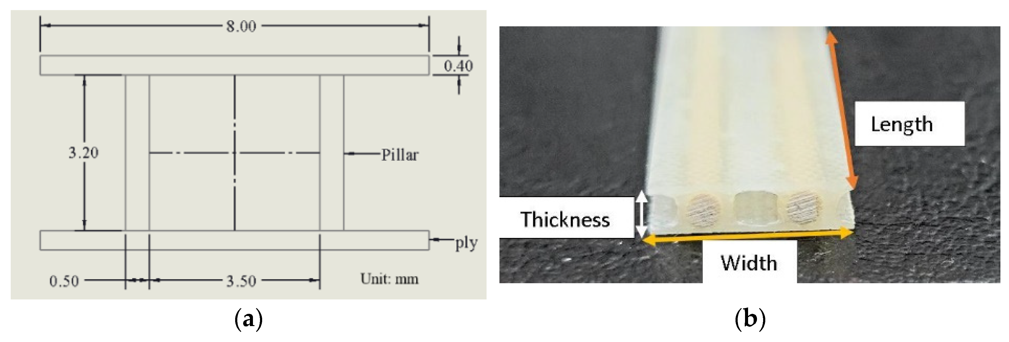
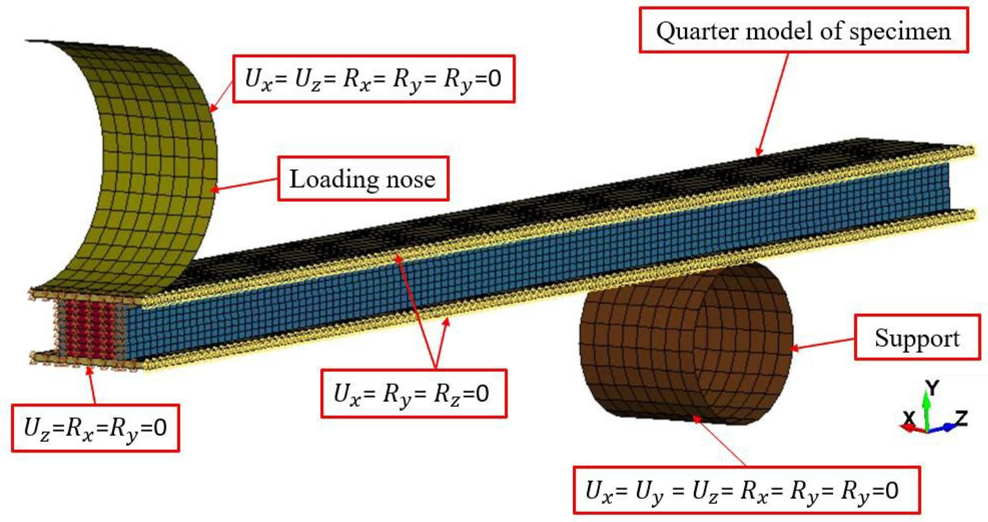
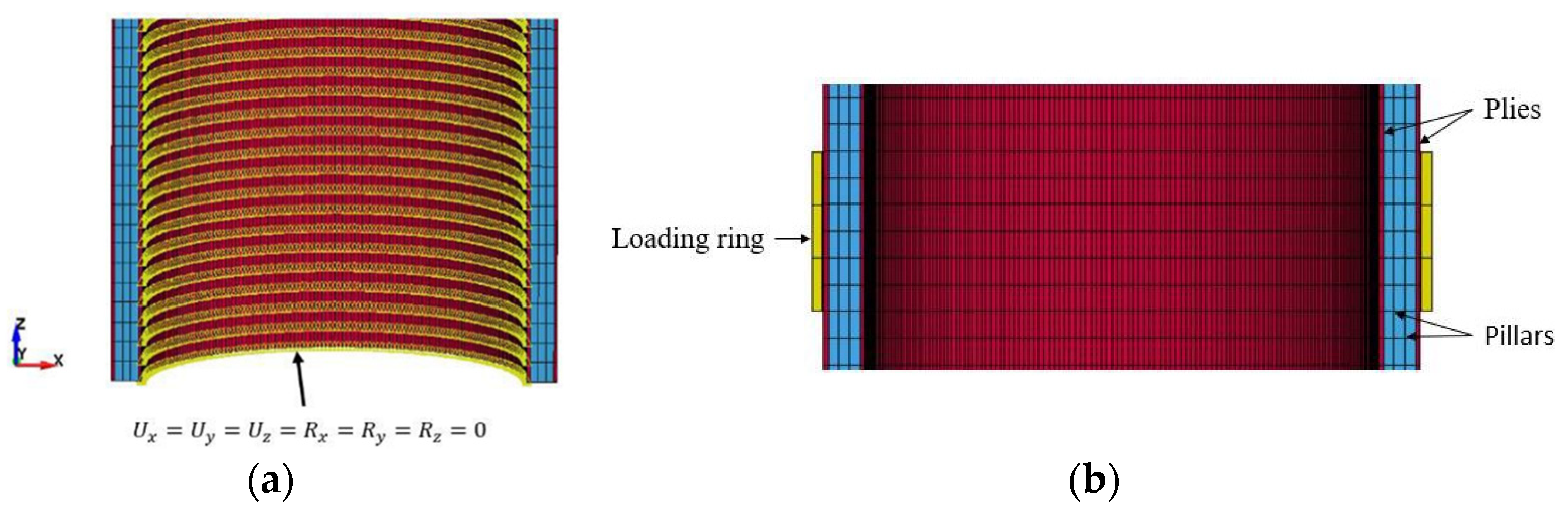
2.1. Simulation of the Behaviour of the Flexural 3DdrFML Specimens
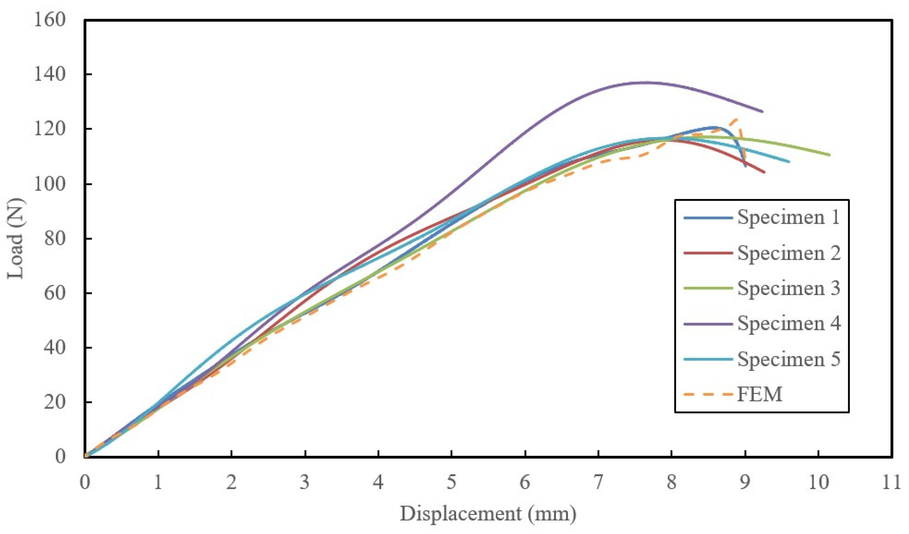
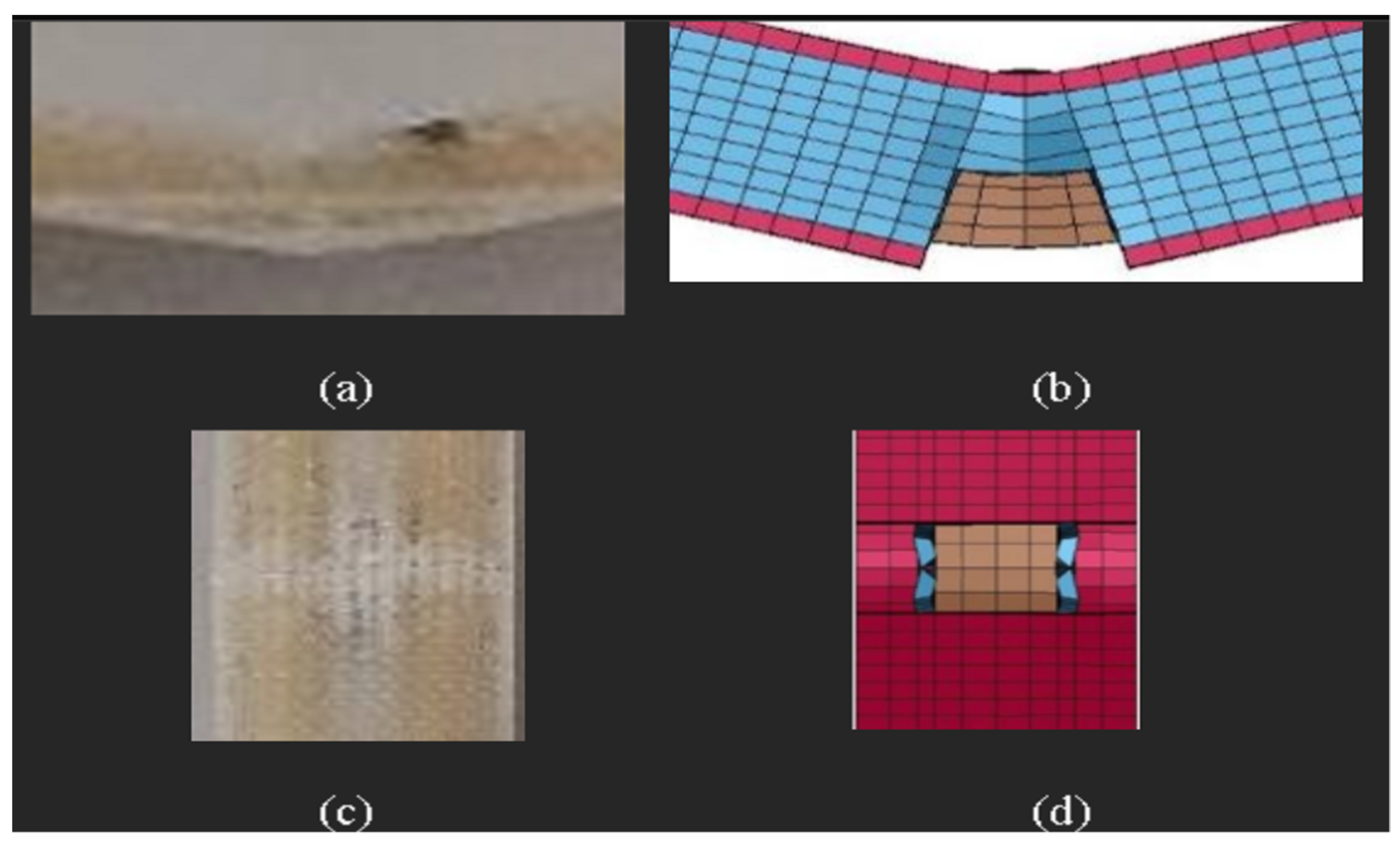
2.2. Results and Discussions
3. Pole Designs
3.1. Preliminary Analyzes
3.1.1. Establishment of an Effective Layup
3.1.2. Influence of Element Formulation
3.2. Design of the Modular Pole Made of 2D Fabric
3.3. Scaled Pole Design
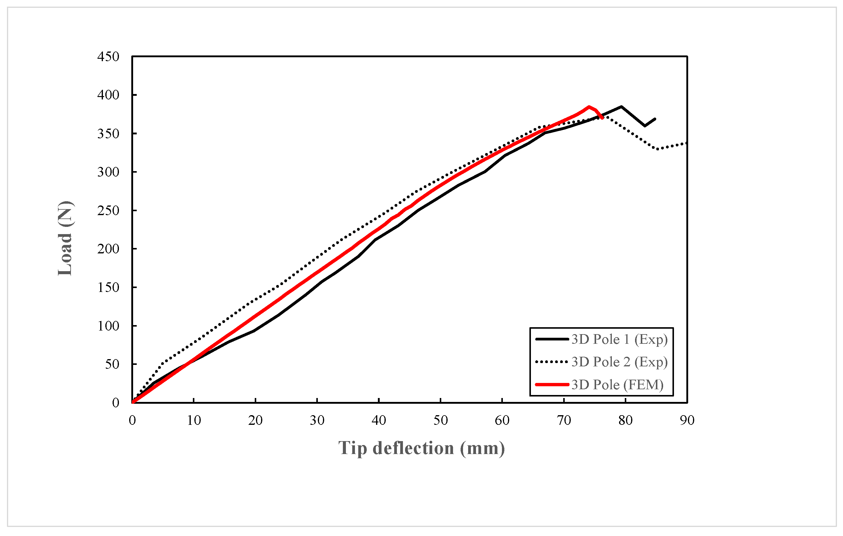
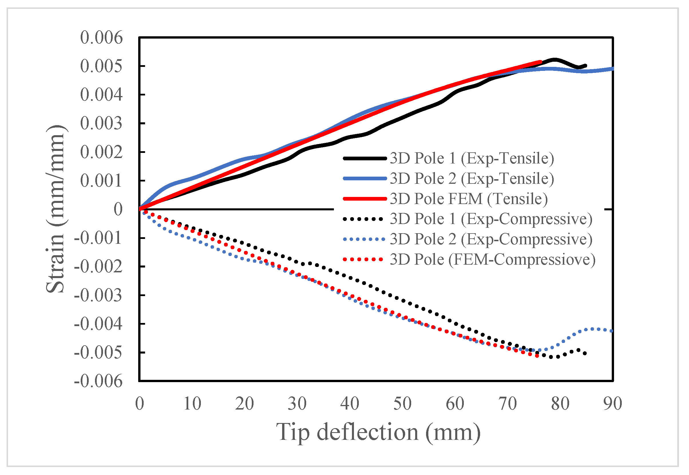
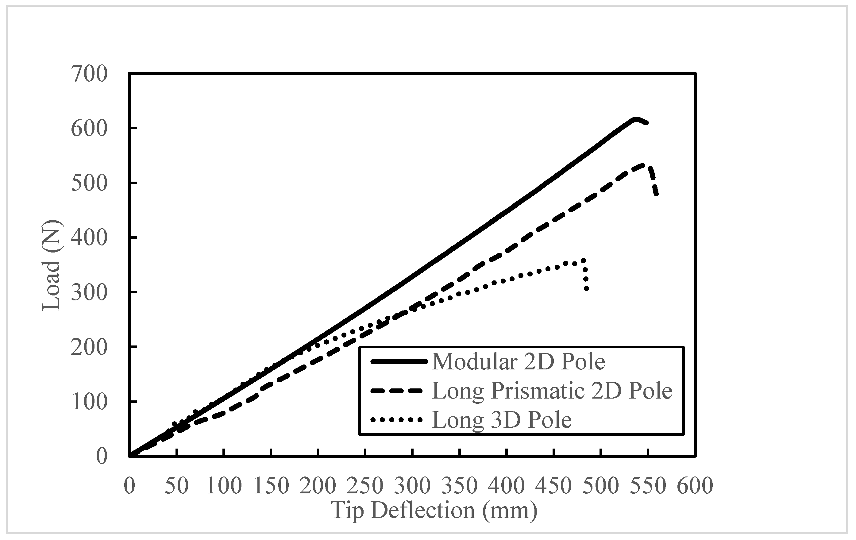
4. Comparison of the Performance of 2D and 3D Poles
5. A Simple Equation for Establishing the Stiffness of 3D Poles
6. Summary and Conclusions
Author Contributions
Funding
Data Availability Statement
Conflicts of Interest
References
- Morrell, J.J. Wood Pole Maintenance Manual; Forest Research Laboratory, Oregon State University: Corvallis, OR, USA, 2012. [Google Scholar]
- R S Technologies Inc. RS Poles 2023. Available online: https://www.rspoles.com/ (accessed on 27 November 2023).
- CSA Group. Overhead Systems. C22.3 No. 1-15 2015. Available online: https://www.scc.ca/en/standardsdb/standards/27989 (accessed on 27 November 2023).
- Recommended Practice for Fiber-Reinforced Polymer Products for Overhead Utility Line Structures, 2nd ed.; Fecht, G. (Ed.) American Society of Civil Engineers (ASCE): Reston, VA, USA, 2019. [Google Scholar]
- Nath, A.; Anand, R.; Desai, J.; Sultan, M.T.H.; Raj, S.A. Modelling and Finite Element Analysis of an Aircraft Wing Using Composite Laminates; IOP Conf. Series: Materials Science and Engineering; IOP Publishing: Bristol, UK, 2021. [Google Scholar] [CrossRef]
- Siefert, A.; Henkel, F.-O. Nonlinear analysis of commercial aircraft impact on a reactor building—Comparison between integral and decoupled crash simulation. In Proceedings of the Transactions, SMiRT 21, New Delhi, India, 6–11 November 2011. [Google Scholar]
- Wu, J.; Taheri, F. Development of a Novel Lightweight Utility Pole using a New Hybrid Reinforced Composite—Part 1: Fabrication & Experimental Investigation. J. Compos. Sci. 2023; in press. [Google Scholar]
- LS-DYNA Keyword User’s Manual, 13th ed.; Livermore Software Technology: Livermore, CA, USA, 2021; Volume I, Available online: https://ftp.lstc.com/anonymous/outgoing/jday/manuals/ls-dyna_971_manual_k_rev1.pdf (accessed on 27 November 2023).
- Mohamed, M.; Taheri, F. Influence of graphene nanoplatelets (GNPs) on mode I fracture toughness of an epoxy adhesive under thermal fatigue. J. Adhes. Sci. Technol. 2017, 31, 19–20. [Google Scholar] [CrossRef]
- LS-DYNA Keyword User’s Manual, 13th ed.; Livermore Software Technology: Livermore, CA, USA, 2021; Volume II, Available online: https://ftp.lstc.com/anonymous/outgoing/jday/manuals/LS-DYNA_Manual_Volume_II_R9.0.pdf (accessed on 27 November 2023).
- Wang, K.; Taheri, F. Compressive Residual Strengths of GLARE and a 3DFML. Polymers 2023, 15, 1723. [Google Scholar] [CrossRef]
- Ross, R. Wood Handbook: Wood as an Engineering Material; Forest Service U.S. Department of Agriculture: Washington, DC, USA, 2021.
- Ekşi, S.; Genel, K. Comparison of Mechanical Properties of Unidirectional and Woven Carbon, Glass and Aramid Fiber Reinforced Epoxy Composites. Acta Phys. Pol. A 2017, 132, 879–882. [Google Scholar] [CrossRef]
- Altanopoulos, T.I.; Raftoyiannis, I.G.; Polyzois, D. Finite element method for the static behavior of tapered poles made of glass fiber reinforced polymer. Mech. Adv. Mater. Struct. 2021, 28, 2141–2150. [Google Scholar] [CrossRef]
- Ibrahim, S.M. Performance Evaluation of Fiber-Reinforced Polymer Poles For Transmission Lines. Ph.D. Thesis, Manitoba University, Winnipeg, MB, Canada, 2000. [Google Scholar]


| Normal Failure Stress (MPa) | Shear Failure Stress (MPa) | Mode I Energy Release Rate (KJ/m2) | Mode II Energy Release Rate (KJ/m2) | Penalty Stiffness (N/mm3) |
|---|---|---|---|---|
| 59 | 23 | 1.5 | 2 | 3500 |
| Upper and lower plies | ρ | E11 | E22 | v21 | G12 | G23 | G31 |
| (g/mm3) | (MPa) | (MPa) | (MPa) | (MPa) | (MPa) | ||
| 0.00175 | 9000 | 9000 | 0.05 | 1000 | 1000 | 1000 | |
| Xc (MPa) | XT (MPa) | Yc (MPa) | YT (MPa) | S12 (MPa) | εT1 | εC1 | |
| 153 | 179 | 153 | 179 | 30 | 0.08 | −0.04 | |
| Pillars | ρ | E11 | E22 | v21 | G12 | G23 | G31 |
| (g/mm3) | (MPa) | (MPa) | (MPa) | (MPa) | (MPa) | ||
| 0.00175 | 3000 | 1000 | 0.05 | 1000 | 1000 | 1000 | |
| Xc (MPa) | XT (MPa) | Yc (MPa) | YT (MPa) | S12 (MPa) | εT1 | εC1 | |
| 80 | 80 | 80 | 80 | 30 | 0.054 | −0.054 | |
| Dowels | ρ | EL | ET | GLT | GLR | v21 | Xc |
| (g/mm3) | (MPa) | (MPa) | (MPa) | (MPa) | (MPa) | ||
| 0.0006 | 11,330 | 974.38 | 1099.01 | 1665.51 | 23,671 | 51.1 | |
| Xc | Yc | Yc | S12 | ||||
| (MPa) | (MPa) | (MPa) | (MPa) | ||||
| 51.1 | 6.5 | 8 | 13.2 |
| Max Load (N) | Max. Disp. (mm) | Ef (MPa) | Flexural Rigidity (N·mm2) | % Error | |
|---|---|---|---|---|---|
| Exp | 134.0 | 8.6 | 10,267.1 | 679,683.3 | |
| 608,273.1 | 10.5 | ||||
| FEM | 128.0 | 8.9 | 9188.42 |
| Elastic Modulus, EC (MPa) | Ultimate Load (N) | Ultimate Strength (MPa) | Ultimate Strain (mm/mm) | % Error in Elastic Modulus | |
|---|---|---|---|---|---|
| Exp | 8963.5 | 2747.0 | 69.5 | 0.015 | 9.9 |
| FEM | 8080.0 | 2556.0 | 61.4 | 0.017 |
| Geometric Features | Length = 2000 mm | ID = 48 mm | Total Thickness = 2.6 |
|---|---|---|---|
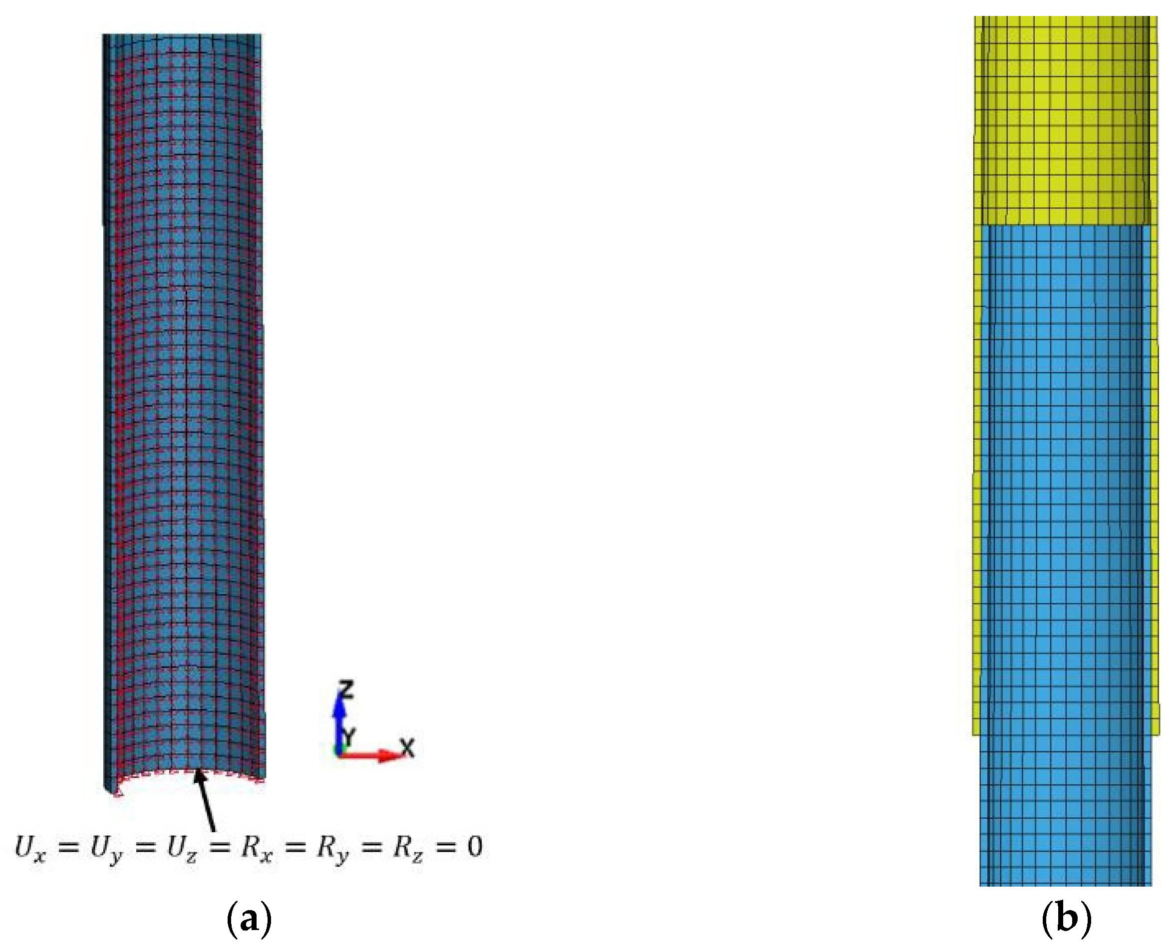
| Boundary conditions | Pole embedment height (mm) | Distance of load from the tip (mm) | Load magnitude (N) |
| 200 | 100 | 793 |
| [+2/05/+2] | [+4/05] | [90/011/90] | [+7] | [013] | [+/09/+] | [+/90/07/90/+] | |
|---|---|---|---|---|---|---|---|
| Longitudinal tension failure | F | F | P | F | P | P | F |
| Transverse tension failure | P | P | F | P | P | P | F |
| In-plane shear failure | F | F | P | F | P | P | F |
| Through-thickness tension failure | F | F | F | F | P | P | F |
| Through-thickness shear failure | P | P | P | P | P | P | F |
| Longitudinal compression failure | F | F | P | F | P | P | F |
| Transverse compression failure | P | P | P | P | P | P | P |
| Through-thickness compression failure | F | P | F | P | P | P | F |
| Solid Elements | Tshell Elements | Analytical | Solid Elements % Error | Tshell Elements % Error | |
|---|---|---|---|---|---|
| Maximum deflection (mm) | 349.3 | 361.8 | 352 | 0.7 | 2.8 |
| Maximum bending stress (MPa) | 133 | 116 | 137.3 | 3.2 | 15.5 |
| CPU Time (s) | 989 | 25 | - | - | - |
| Module | Length (mm) | Upper Dia. (mm) | Lower Dia. (mm) | Thickness (mm) | Taper Angle (Deg.) | Overlap Length |
|---|---|---|---|---|---|---|
| Upper | 1000 | 47.2 | ||||
| 54.2 | 2.6 | 0.2 | 135.2 | |||
| Lower | 880 | 48.1 |
| Proposed Design (Assembled) | RS Technologies | Pole of Ref. [14] | Pole of Ref. [15] | |
|---|---|---|---|---|
| Slenderness ratio | 165.7 | 219.2 | 127.7 | 83.0 |
| Davg/t | 20.7 | 27.5 | 19.4 | 65.5 |
| Fabric Type | ρ (g/mm3) | E11 (MPa) | E22 (MPa) | v21 | G12 (MPa) | G23 (MPa) | G31 (MPa) |
| 0.00175 | 15,560 | 6749 | 0.11 | 3310.8 | 2595.8 | 3310.8 | |
| UD | Xc (MPa) | XT (MPa) | Yc (MPa) | YT (MPa) | S12 (MPa) | ||
| 343.3 | 572.2 | 80.1 | 78 | 30.9 | |||
| ρ (g/mm3) | E11 (MPa) | E22 (MPa) | v21 | G12 (MPa) | G23 (MPa) | G31 (MPa) | |
| Biaxial [+] | 0.00175 | 9336 | 4049.4 | 0.11 | 1986.4 | 1557.5 | 1655.4 |
| Xc (MPa) | XT (MPa) | Yc (MPa) | YT (MPa) | S12 (MPa) | |||
| 223.1 | 343.3 | 48.1 | 46.8 | 18.5 |
| Moment of inertia, I (mm4) | Ex (MPa) | Stiffness (N·mm2) | % Error in Ex | |
|---|---|---|---|---|
| Experiment | 115,149.5 | 9726.5 | 1.12 × 10⁹ | 0.89 |
| FEM | 9639.6 | 1.11 × 10⁹ |
| Pole Type | Volume (mm3) | Mass (g) | Stiffness (N·mm2) | Ultimate Load Capacity (N) | Normalized Ultimate Load Capacity (N/kg) |
|---|---|---|---|---|---|
| 2D Pole | 68,6711 | 760.5 | 1.02 × 10⁹ | 616.0 | 0.81 |
| 2D Prismatic Pole | 57,2920 | 634.5 | 9.02 × 10⁸ | 530.0 | 0.84 |
| Long Prismatic 3D Pole | 66,9842 | 729.2 | 1.06× 10⁹ | 355.8 | 0.49 |
| Method | Extensional Elastic Modulus (MPa) | Stiffness (N·mm2) | % Error in Stiffness |
|---|---|---|---|
| Experimental value (Compression Test) | 8963.5 | 152,208 | |
| Equation (1) | 8686.0 | 152,154 | 0.03 |
| Equation (2) | 5296.0 | 152,154 |
Disclaimer/Publisher’s Note: The statements, opinions and data contained in all publications are solely those of the individual author(s) and contributor(s) and not of MDPI and/or the editor(s). MDPI and/or the editor(s) disclaim responsibility for any injury to people or property resulting from any ideas, methods, instructions or products referred to in the content. |
© 2024 by the authors. Licensee MDPI, Basel, Switzerland. This article is an open access article distributed under the terms and conditions of the Creative Commons Attribution (CC BY) license (https://creativecommons.org/licenses/by/4.0/).
Share and Cite
Wu, Q.; Taheri, F. Development of a Novel Lightweight Utility Pole Using a New Hybrid Reinforced Composite—Part 2: Numerical Simulation and Design Procedure. J. Compos. Sci. 2024, 8, 50. https://doi.org/10.3390/jcs8020050
Wu Q, Taheri F. Development of a Novel Lightweight Utility Pole Using a New Hybrid Reinforced Composite—Part 2: Numerical Simulation and Design Procedure. Journal of Composites Science. 2024; 8(2):50. https://doi.org/10.3390/jcs8020050
Chicago/Turabian StyleWu, Qianjiang, and Farid Taheri. 2024. "Development of a Novel Lightweight Utility Pole Using a New Hybrid Reinforced Composite—Part 2: Numerical Simulation and Design Procedure" Journal of Composites Science 8, no. 2: 50. https://doi.org/10.3390/jcs8020050