Predicting the Dynamic Parameters for Milling Thin-Walled Blades with a Neural Network

Abstract

Accurately predicting the time-varying dynamic parameters of a workpiece during the milling of thin-walled parts is the foundation of adaptively selecting chatter-free machining parameters. Hence, a method for accurately and quickly predicting the time-varying dynamic parameters for milling thin-walled parts is proposed, which is based on the shell FEM and a three-layer neural network. The time-dependent dynamics of the workpiece can be calculated using the FEM by obtaining the geometrical parameters of the arc-faced junctions within the discrete cells of the initial and machined workpiece. It is unnecessary to re-divide the mesh cells of the thin-walled parts at each cutting position, which enhances the computational efficiency of the workpiece dynamics. Meanwhile, in comparison with the three-dimensional cube elements, the shell elements can reduce the number of degrees of freedom of the FEM model by 74%, which leads to the computation of the characteristic equation that is about nine times faster. The results of the modal test show that the maximum error of the shell FEM in predicting the natural frequency of the workpiece is about 4%. Furthermore, a three-layer neural network is constructed, and the results of the shell FEM are used as samples to train the model. The neural network model has a maximum prediction error of 0.409% when benchmarked against the results of the FEM. Furthermore, the three-layer neural network effectively enhances computational efficiency while guaranteeing accuracy.

1. Introduction

To reduce the weight of aircraft and spacecraft, thin-walled parts have been widely used in the aerospace industry, such as in aircraft engine casings and blades. The machining of thin-walled parts is mainly carried out through machining and non-traditional energy-assisted machining methods [1], but machining is still the main material removal process for the vast majority of aerospace parts as non-traditional methods are affected by efficiency and quality control. The structural characteristics of thin-walled parts make them prone to chatter during CNC machining, thereby leading to machining defects on the surface of parts. This results in difficulties in achieving the required machining precision and surface integrity for the machined parts. To select reasonable machining parameters, the dynamic modeling of thin-walled parts is required to calculate the stable machining parameter domain. However, due to material removal, the machining system of thin-walled parts exhibits strong time-varying behavior; therefore, it is necessary to obtain the dynamic parameters during the machining process of thin-walled parts. It would be very time-consuming to use the finite element method to calculate the dynamic parameters of a thin-walled part at any tool position. In this paper, a finite element model based on shell elements is developed to obtain the workpiece thickness and dynamic parameter datasets, which are then used to train a neural network model to highly improve computational efficiency while ensuring prediction accuracy.

There are already some results from studies on the prediction of the time-varying kinetic parameters for cutting thin-walled parts. After using modal tests to obtain the kinetic parameters of thin-walled parts at different cutting steps, Bravo et al. [2] point out that the variation in workpiece kinetic parameters affects the milling stability limit of thin-walled parts. However, since it is somewhat time-consuming to frequently repeat tests on the workpiece during the cutting process, the authors were subsequently prompted to choose numerical methods instead of investigating the effect of the workpiece dynamic parameter variation on the milling stability. Seguy et al. [3] use the finite element method (FEM) to study the evolution of workpiece dynamic parameters during the milling process. Arnaud et al. [4] analyze the variation in workpiece kinetic parameters during the cutting process through finite element analysis and investigate the impact of material removal and cutting position on the chatter-free boundary. Thevenot et al. [5] use both experimental tests and finite element modeling to investigate the variation in workpiece kinetic parameters during machining. Song et al. [6] first correct the finite element calculation values using experiment data, and then, with the corrected finite element model, they manage to establish the cutting dynamic equations that take into account the time-varying nature of the workpiece kinetic parameters. This method guarantees prediction accuracy as long as the boundary conditions of the model are correctly defined. However, since reconstructing the finite element model and re-computing the modal analysis are to a certain degree quite time-consuming, several algorithms have been proposed by scholars to avoid the frequent modeling and meshing of the finite element model of the workpiece as well as to improve the computational efficiency of the workpiece kinetic parameters. Meshreki et al. [7] propose an analytical model for calculating the kinetic parameters of thin-walled parts during milling, taking into account the variation in the workpiece thickness. Song et al. [8] opt for the Sherman–Morrison–Woodbury equation to predict the Frequency Response Functions (FRFs) of the workpiece during the milling process of thin-walled parts. Moreover, Song et al. [9] also propose a spatio-temporal discrete method for milling the stability prediction of thin-walled parts based on thin-plate theory and the principle of modal superposition, which take into account the influence of the tool–workpiece engagement position and the system’s multimodal state. Ahmadi [10] applies FSMs (Finite Strip Models) to obtain the kinetic parameters of the workpiece during the milling process of frame structures. Tuysuz et al. [11] propose a process model for updating the kinetic parameters of the workpiece in the frequency domain, which is based on complete- and reduced-order dynamic substructures.

All the aforementioned studies are conducted on flat-plate-like structures. In terms of the machining of surfaced parts, Yang et al. [12] propose a method to calculate the workpiece modal parameters when the tool cuts at an arbitrary position that is based on structural modal parameter modification, which only calculates the modal vibration patterns and natural frequencies of the workpiece during machining through the modal analysis of the initial workpiece’s FEM model without re-modeling or re-meshing the workpiece used for each cutting state. Subsequently, they investigate the effect of time-varying modal parameters on the milling stability of thin-walled parts. Yang et al. [13] put forth a decomposition–condensation method to predict the modal parameters of a workpiece for the finishing/semi-finishing of a large thin-walled workpiece. The method decomposes the workpiece into the machined workpiece and the material to be removed using structural dynamic modification techniques to update the time-varying model of the material to be removed, through which the reconstruction of the finite element model of the workpiece is avoided. Dang et al. [14] advance a method combining the degree of freedom reduction and structural modification techniques to calculate the FRFs of a workpiece that is used in machining, which aims to reduce the degree of freedom of the workpiece’s mass matrix and stiffness matrix during machining. After that, they look into the impact of tool position and material removal on modal parameters such as the workpiece natural frequency and modal vibration pattern, and they establish three-dimensional stability lobe diagrams for the milling of flat thin-walled and surfaced thin-walled parts.

For the machining of complex curved-blade parts, Budak et al. [15] utilize commercial finite element software to build a finite element model of the blade structure based on 3D cubic cells to obtain the initial FRFs of the workpiece. They update the workpiece modal parameters with the cells removed during the machining process. Zhang et al. [16] choose the matrix perturbation method to calculate the modal parameters of the blade structure. Luo et al. [17] apply numerical simulations to study the evolution of workpiece modal parameters and cutting stability during the milling of thin-walled blades. Tian et al. [18] calculate the natural frequency of the workpiece during the process of thin-walled blade milling with the matrix perturbation method. Ju [19] delve into the multi-axis milling of thin-walled parts with variable levels of thickness on complex surfaces. The entire machining process is discretized into a finite number of elements along the tool path, and the cutting process is viewed as a process of removing each discrete element one by one. The Sherman–Morrison–Woodbury formula is later applied to predict the variation in the workpiece modal parameters during the machining process. Tuysuz et al. [20] introduce a model for predicting instantaneous modal parameters of blade parts during the cutting process based on reduced structural matrix decoupling and modal mode perturbation, verifying the proposed model through cutting experiments and FRFs testing. With an analytical method, Liu [21] seeks to solve the variation in workpiece modal parameters during impeller blade machining based on theoretical mechanics and the shallow shell theory.

To sum up, the literature [2,3,4,5,6,7,8,9,10,11] focuses on flat-plate structures. In terms of the curved blades, the literature [17,18] attempts to simplify the curved-blade structure to a flat-plate one. However, there is a significant discrepancy in the mechanical properties between flat-plate structures and curved-blade parts, which can lead to significant calculation errors. The literature [15] employs three-dimensional cubic elements for the finite element modeling of thin-walled blades, which results in the large model of degrees of freedom. Additionally, it is time-consuming to simulate and analyze the cutting process using finite element software. The method proposed in the literature [21] inherently presumes a vibration equation to the workpiece based on boundary conditions. There will be a significant computational mistake if the assumed vibration that is equation is unreasonable. The study yields a maximum error of 8% for the first two modal natural frequencies. Based on the matrix perturbation method, the literature [15] predicts the natural frequency of blade structures with a maximum error of 7.3%, which is relatively high. To implement the curved-blade machining requirements, it is necessary to establish a workpiece modal parameter prediction model that factors in the blade’s surface characteristics and ensures both calculation accuracy and efficiency. Currently, machine learning is widely used in various fields such as system identification, pattern recognition, and intelligent control [22]. Its highly robust and fault-tolerant ability allows for the adequate approximation of complex nonlinear relationships.

At present, neural networks have been widely used for predicting cutting force, tool wear, and workpiece surface roughness [23,24,25,26,27]. Yeganefar et al. [23] predicted and optimized the surface roughness and cutting forces in the slot milling of a 7075-T6 aluminum alloy using regression analysis, support vector regression (SVR), artificial neural network (ANN), and multivariate analysis methods. The effect of the process parameters, including cutting speed, feed per tooth, depth of cut, and tool type, on the response was investigated by analysis of variance (ANOVA). Pavlenko et al. [24] evaluated the effect of the process parameters on the power characteristics of the cutting process in cylindrical feed grinding based on artificial neural network (ANN) and multiparameter proposed linear regression analysis methods as well as numerical experiments in order to investigate the cutting force and evaluate the key indicators of the cutting force. SK et al. [25] used an artificial neural network approach to accurately predict the back face wear of a tool based on the response of the cutting force and surface roughness. Vasanth et al. [26] predicted the surface roughness by using a regression model and an artificial neural network model to fuse the cutting force, cutting temperature, tool wear, and vibrational displacements of the tool, which showed that the predicted surface roughness was better than that predicted by a multi-parameter proposed linear regression analysis and multi-parameter proposed linear regression analysis. The results show that the predicted surface roughness is more accurate than that of the regression model. Wang et al. [27] predicted the cutting force by using a neural network approach and built a “transmission network” based on the data obtained from the simulation. Compared with the “normal network”, the transmission network has obvious performance advantages. Heitz1 et al. [28] used model training as a new feature of the mechanical force model in the time and frequency domains, and the cutting force was predicted efficiently by the extreme gradient boosting optimization algorithm, which improved the optimization accuracy, efficiency, user-friendliness, and efficiency. Currently, machine learning neural network models are rarely studied for modal parameter predictions.

Hence, a method that is based on both the shell FEM and a three-layer neural network and that also considers workpiece geometry is proposed for predicting the time-varying dynamics during the milling of the thin-walled curved-blade structure. The built FEM based on shell elements only needs to mesh the initial workpiece and the machined workpiece once, and it only needs to calculate the geometric parameters of the initial workpiece and the machined workpiece. It does not need to re-mesh the thin-walled parts at each cutting position nor to repeatedly calculate the geometric parameters of the workpiece during the cutting process. Meanwhile, in comparison with the three-dimensional cube elements used in reference [15], the shell elements can reduce the number of degrees of freedom of the FEM and improve computing efficiency. Meanwhile, a three-layer neural network model is constructed to predict the time-varying dynamic parameters for milling the thin-walled parts. The three-layer neural network model can highly improve calculation efficiency while ensuring calculation accuracy.

A dynamic model is established in Section 1 for the milling of the thin-walled blades. In Section 2, a shell unit-based time-varying dynamic parameter prediction model is constructed for the milling of the thin-walled parts. In Section 3, a three-layer neural network model is constructed to achieve the prediction of the time-varying kinetic parameters for milling the thin-walled parts. In Section 4, the validity of the shell unit finite element model is verified through modal test experiments. Meanwhile, the neural network model is trained using the calculation results of the shell unit finite element model as training samples, and the calculation results of the neural network model and the shell unit finite element model are compared and analyzed.

2. Modeling of Thin-Walled Blade Dynamics Based on the Removal Process

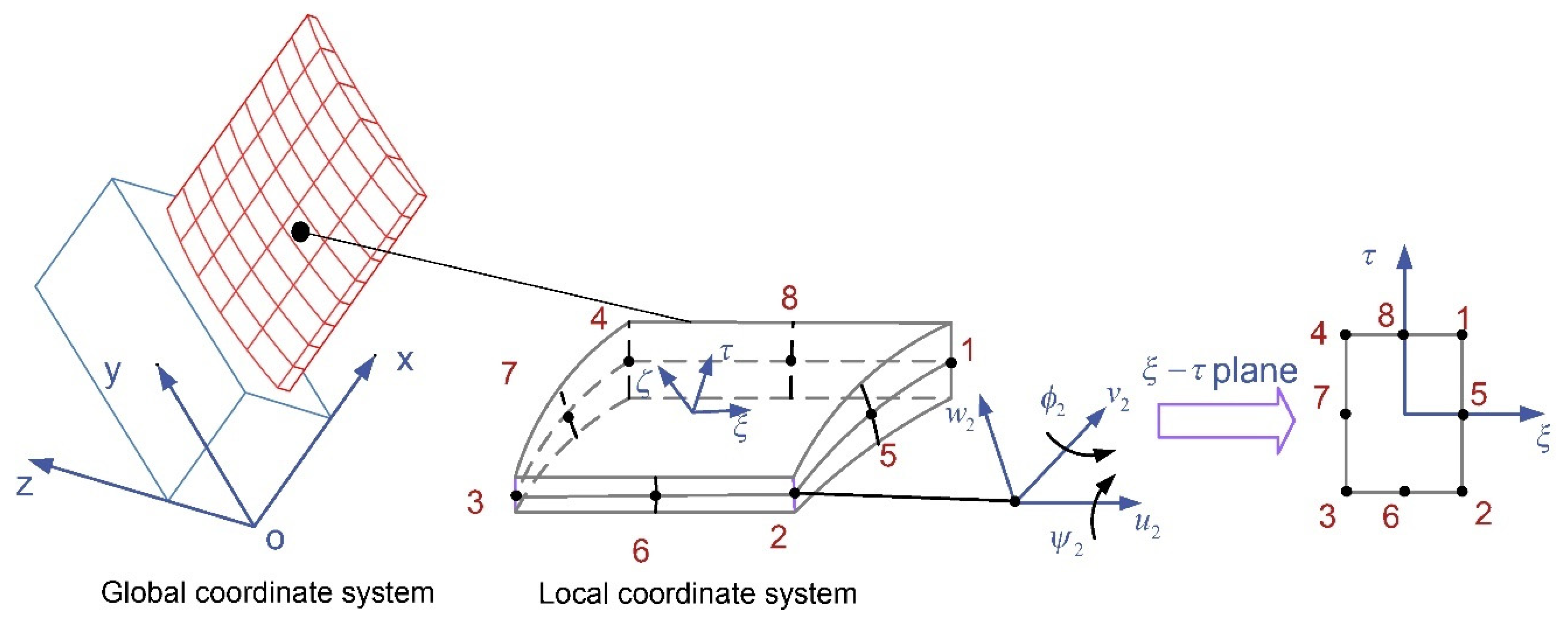
2.1. Dynamic Model of the Thin-Walled Blade Structure

Aviation blades are structurally characteristic of their thin-walled parts, and the cross-section thickness varies significantly along the chord direction, which makes it challenging to characterize their structural characteristics through specific geometric parameters. Analyzing this type of continuous medium dynamic problem requires the discretization of the spatial region using the finite element method to obtain a discretized multi-degree-of-freedom dynamic model, as shown in Figure 1.

The structural dynamic equations of the discretized model of the blade in the physical coordinate system can be put as follows:

$$M\ddot{u}+C\dot{u}+Ku=0$$

(1)

where $u$, $\dot{u}$, and $\ddot{u}$ denote the displacement vector, velocity vector, and acceleration vector, respectively. $M$, $C$, and $K$, respectively, stand for the mass matrix, damping matrix, and stiffness matrix of the workpiece. If the workpiece’s damping is disregarded, the aforementioned equation can be simplified as follows:

$$M\ddot{u}+Ku=0$$

(2)

The characteristic equation of Equation (2) can be written as follows:

$$(K-\lambda M)\mathsf{\Phi }=0$$

(3)

where $\lambda$ and $\mathsf{\Phi }$ denote the eigenvalues and eigenvectors of the eigenequations. The blade structure’s nature frequency $\omega$, and its corresponding mode shapes are $\sqrt{\lambda }$ and $\mathsf{\Phi }$, respectively.

The complete process constitutes the continuous removal of the blade material from semi-finishing to the end of finishing. When meshing the blade body, the structural properties of the original workpiece state can be expressed in terms of the mass matrix $M_0$, stiffness matrix $K_0$, eigenvalues, and eigenvectors ${\mathsf{\Phi }}_0$. Hence, the workpiece nature frequency and modal formation can be expressed as:

$$K_0{\mathsf{\Phi }}_{i0}={\lambda }_{i0}{M}_0{\mathsf{\Phi }}_{i0}\hspace{1em}\hspace{1em}(i=1~n)$$

(4)

The material removal process can be considered as a continuous removal process of a number of grid cells on the original conditions of the workpiece, and the amount of change in the mass and stiffness induced by a number of grid cells can be represented as $\Delta K$, $\Delta M$. After resection is complete, the mass and stiffness matrices of the new process system can be put as follows:

$$K=K_0-\Delta K; M=M_0-\Delta M$$

(5)

The structural properties of the modified system can be stated as follows:

$$(K_0-\Delta K)x_i=\lambda (M_0-\Delta M)x_i$$

(6)

2.2. Milling Process Grid Cell Definitions

Due to its unique structural properties, the wall thickness of the blade is significantly less than 1/10 of the total structural size of the blade. Using the shell unit can simplify the three-dimensional geometric structure by extracting the mid-plane, provided that the stress along the thickness direction is neglected. It can highly reduce the solution scale and improve the calculation efficiency while maintaining geometrical accuracy. Therefore, shell units are used herein to simulate the structural characteristics of thin-walled blades, and the original 3D eight-node hexahedron is converted into a 2D first-order planar body unit by extracting the mid-plane, as illustrated in Figure 2.

To further describe the change process of the structural parameters of the material removal process when milling thin-walled blades, a novel approach is proposed herein to divide the workpiece into three categories including initial workpiece, workpiece during the cutting process, and machined workpiece. Additionally, the cutting process workpiece is divided into two parts as follows: the uncut part and the machined part, as shown in Figure 3.

The same discrete cell form is then used to mesh the three states of the workpiece. Subsequently, the geometrical parameters of the arc-face nodes in the discrete cells of the initial and machined workpiece are calculated. By combining the corresponding discrete cells of the initial and machined workpiece, it is possible to obtain the geometrical parameters of the discrete cell nodes of the workpiece during the cutting process. Then, the stiffness and mass matrices of the discrete units of the workpiece during the cutting process are constructed by the shell unit, and, lastly, the overall stiffness and mass matrices of the workpiece during the cutting process are obtained by synthesis, and the workpiece’s time-varying dynamic parameters are calculated. To improve the efficiency of the calculation of the kinetic parameters of the workpiece, this method only needs to mesh the initial workpiece and the processed workpiece once and calculate the geometric parameters of the initial workpiece and the processed workpiece. It also dispenses with the need to re-divide the mesh cells of the thin-walled parts and repeat the calculation of the workpiece geometric parameters during the cutting process at each cutting position. The specific synthesis process is as follows.

Based on the above finite element idea, the discretized unit stiffness matrix and mass matrix are represented as follows using the dynamic equations [29]:

$$\left\{\begin{array}{l}{K}_{le}((x_i,y_i,z_i),t_i,m_i)={\displaystyle {\int }_{-1}^1{\displaystyle {\int }_{-1}^1{\displaystyle {\int }_{-1}^1{B}^{T}DB\left|J\right|d\xi d\tau d\zeta }}}\\ M_{le}((x_i,y_i,z_i),t_i,m_i)={\displaystyle {\int }_{-1}^1{\displaystyle {\int }_{-1}^1{\displaystyle {\int }_{-1}^1\rho N^{T}N\left|J\right|d\xi d\tau d\zeta }}}\end{array}\right.,(i=1,2,\cdots ,8)$$

(7)

where $\rho$ signifies the density of the workpiece and the elasticity matrix $D$ is expressed as follows:

$$D=\frac{E}{1-{\mu }^2}\left[\begin{array}{ccccc}1& \mu & 0& 0& 0\\ \mu & 1& 0& 0& 0\\ 0& 0& \frac{1-\mu }{2}& 0& 0\\ 0& 0& 0& \frac{1-\mu }{2k}& 0\\ 0& 0& 0& 0& \frac{1-\mu }{2k}\end{array}\right]$$

(8)

where $E$ is the modulus of elasticity, $\mu$ is Poisson’s ratio, and the coefficient $k$ is introduced to account for the impact of the inhomogeneity of the shear stresses and takes the value of 1.2. From Equation (7), it is evident that to compute the mass and stiffness matrices of the discrete shell cell, it is necessary to define the matrices of $J$, $N$, and $B$. The matrices $J$, $N$, and $B$ are defined as follows:

Define the matrix $J$: The global coordinates of any point within the shell cell in the global coordinate system can be represented as follows:

$$\left\{\left.\begin{array}{l}x\\ y\\ z\end{array}\right\}\right.={\displaystyle \sum _{i=1}^8{N}_i}{\left\{\left.\begin{array}{l}{x}_i\\ y_i\\ z_i\end{array}\right\}\right.}_{MID}+{\displaystyle \sum _{i=1}^8{N}_i}\frac{\zeta }{2}\left\{\left.\begin{array}{l}{H}_{3i}(1)·t_i\\ H_{3i}(2)·t_i\\ H_{3i}(3)·t_i\end{array}\right\}\right.$$

(9)

where $N_i$ signifies the cell shape function, $MID$ the shell cell midplane, $(x_i,y_i,z_i)$ the coordinates of the nodes on the midplane of the shell cell, $H_{3i}$ the midplane normal vector, and $t_i$ the shell cell thickness. For the cell node numbering shown in Figure 1, the cell shape function can be put as follows:

$$\left\{\begin{array}{l}{N}_1=\frac{1}{4}(1+\xi )(1+\tau )(\xi +\tau -1),N_2=\frac{1}{4}(1+\xi )(1-\tau )(\xi -\tau -1)\\ N_3=\frac{1}{4}(1-\xi )(1-\tau )(-\xi -\tau -1),N_4=\frac{1}{4}(1-\xi )(1+\tau )(-\xi +\tau -1)\\ N_5=\frac{1}{2}(1+\xi )(1-{\tau }^2),N_6=\frac{1}{2}(1-{\xi }^2)(1-\tau )\\ N_7=\frac{1}{2}(1-\xi )(1-{\tau }^2),N_8=\frac{1}{2}(1-{\xi }^2)(1+\tau )\end{array}\right.$$

(10)

The Jacobi matrix $J$ is defined as:

$$J=\left[\begin{array}{ccc}\frac{\partial x}{\partial \xi }& \frac{\partial y}{\partial \xi }& \frac{\partial z}{\partial \xi }\\ \frac{\partial x}{\partial \tau }& \frac{\partial y}{\partial \tau }& \frac{\partial z}{\partial \tau }\\ \frac{\partial x}{\partial \zeta }& \frac{\partial y}{\partial \zeta }& \frac{\partial z}{\partial \zeta }\end{array}\right]$$

(11)

Define the matrix $N$: The shell cell node $i$ has three angular displacements and two linear displacements. Construct the three orthogonal vectors $H_{1i}$, $H_{2i}$, and $H_{3i}$ to define the angular displacements of node $i$. $H_{3i}$ denotes the vector normal to the midplane of the cell at node $i$, and $H_{2i}$ and $H_{3i}$ are two vectors that are tangent to the midplane and perpendicular to the vector and can be constructed in the following form:

$$H_{2i}=H_{3i}\times i(x-axis),H_{1i}=H_{2i}\times H_{3i}$$

(12)

Then, we can obtain the directional cosines $l_{1i}$, $m_{1i}$, $n_{1i}$ of vector $H_{1i}$, the directional cosines $l_{2i}$, $m_{2i}$, $n_{2i}$ of vector $H_{2i}$, and the directional cosines $l_{3i}=H_{3i}(1)$, $m_{3i}=H_{3i}(2)$ and $n_{3i}=H_{3i}(3)$ of vectors $H_{3i}$. Subsequently, the node displacements ${\delta }_i={\left[u_i, v_i, w_i, {\phi }_i, {\psi }_i\right]}^T$ and the cell shape function $N_i\left(\xi , \tau \right)$ can be used to compute the displacements of any point within the cell, defining the matrix $N$ as follows:

$$N=\left[\begin{array}{cccccc}{N}_1& 0& 0& \frac{\zeta N_1{t}_1}{2}{l}_{11}& \frac{\zeta N_1{t}_1}{2}{l}_{21}& \cdots \\ 0& N_1& 0& \frac{\zeta N_1{t}_1}{2}{m}_{11}& \frac{\zeta N_1{t}_1}{2}{m}_{21}& \cdots \\ 0& 0& N_1& \frac{\zeta N_1{t}_1}{2}{n}_{11}& \frac{\zeta N_1{t}_1}{2}{n}_{21}& \cdots \end{array}\right.\left.\begin{array}{ccccc}{N}_8& 0& 0& \frac{\zeta N_8{t}_8}{2}{l}_{18}& \frac{\zeta N_8{t}_8}{2}{l}_{28}\\ 0& N_8& 0& \frac{\zeta N_8{t}_8}{2}{m}_{18}& \frac{\zeta N_8{t}_8}{2}{m}_{28}\\ 0& 0& N_8& \frac{\zeta N_8{t}_8}{2}{n}_{18}& \frac{\zeta N_8{t}_8}{2}{n}_{28}\end{array}\right]$$

(13)

Defining the Geometric Matrix $B$: To calculate the strain of the shell unit in the local coordinate system, it is necessary to construct the local coordinate system. The local coordinate system axes can be constructed in the following form:

$$z\prime =N_1{H}_{31}+N_2{H}_{32}+\cdots +N_8{H}_{38}$$

(14)

where the $y^{\prime }$ and $x^{\prime }$ axes are expressed as follows:

$$y^{\prime }=z^{\prime }\times x=\left|\begin{array}{ccc}i& j& k\\ l_3& m_3& n_3\\ 1& 0& 0\end{array}\right|,x^{\prime }=z^{\prime }\times y^{\prime }$$

(15)

Then, the direction cosines $l_3$, $m_3$, $n_3$ of the axis $z^{\prime }$; the direction cosines $l_2$, $m_2$, $n_2$ of the axis $y^{\prime }$; and the direction cosines $l_1$, $m_1$, $n_1$ of the axis $x^{\prime }$ can be calculated.

The components of the geometric matrix are defined as follows:

$$B_i=\left[\begin{array}{ccccc}{l}_1{\alpha }_1& m_1{\alpha }_1& n_1{\alpha }_1& {\beta }_1{\gamma }_1& {\beta }_1{\lambda }_1\\ l_2{\alpha }_2& m_2{\alpha }_2& n_2{\alpha }_2& {\beta }_2{\gamma }_2& {\beta }_2{\lambda }_2\\ l_1{\alpha }_2+l_2{\alpha }_1& m_1{\alpha }_2+m_2{\alpha }_1& n_1{\alpha }_2+n_2{\alpha }_1& {\beta }_1{\gamma }_2+{\beta }_2{\gamma }_1& {\beta }_1{\lambda }_2+{\beta }_2{\lambda }_1\\ l_2{\alpha }_3+l_3{\alpha }_2& m_2{\alpha }_3+m_3{\alpha }_2& n_2{\alpha }_3+n_3{\alpha }_2& {\beta }_2{\gamma }_3+{\beta }_3{\gamma }_2& {\beta }_2{\lambda }_3+{\beta }_3{\lambda }_2\\ l_3{\alpha }_1+l_1{\alpha }_3& m_3{\alpha }_1+m_1{\alpha }_3& n_3{\alpha }_1+n_1{\alpha }_3& {\beta }_3{\gamma }_1+{\beta }_1{\gamma }_3& {\beta }_3{\lambda }_1+{\beta }_1{\lambda }_3\end{array}\right]$$

(16)

The parameters in Equation (16) are as follows:

$$\left\{\begin{array}{l}{\alpha }_s=l_s\frac{\partial N_i}{\partial x}+m_s\frac{\partial N_i}{\partial y}+n_s\frac{\partial N_i}{\partial z}\\ {\beta }_s=(l_s\frac{\partial P_i}{\partial x}+m_s\frac{\partial P_i}{\partial y}+n_s\frac{\partial P_i}{\partial z})\frac{t_i}{2}\\ {\gamma }_s=l_s{l}_{1i}+m_s{m}_{1i}+n_s{n}_{1i}\\ {\lambda }_s=l_s{l}_{2i}+m_s{m}_{2i}+n_s{n}_{2i}\end{array}\right.$$

(17)

where $P_i=N_i\zeta$. The geometric matrix is denoted as $B=\left[B_1 B_2 \cdots B_8\right]$.

Matrix combination of cells: To derive the mass and stiffness matrices of the blade structure, it is important to transform the matrices obtained from Equation (17) in the local coordinate system to the global coordinate system. The transformation matrix is expressed as follows:

$$\begin{gathered} L=\left[\begin{array}{cccccccc}{\gamma }_1& 0& 0& 0& 0& 0& 0& 0\\ 0& {\gamma }_2& 0& 0& 0& 0& 0& 0\\ 0& 0& {\gamma }_3& 0& 0& 0& 0& 0\\ 0& 0& 0& {\gamma }_4& 0& 0& 0& 0\\ 0& 0& 0& 0& {\gamma }_5& 0& 0& 0\\ 0& 0& 0& 0& 0& {\gamma }_6& 0& 0\\ 0& 0& 0& 0& 0& 0& {\gamma }_7& 0\\ 0& 0& 0& 0& 0& 0& 0& {\gamma }_8\end{array}\right] \\ {\gamma }_i=\left[\begin{array}{ccccc}{l}_{1i}& m_{1i}& n_{1i}& 0& 0\\ l_{2i}& m_{2i}& n_{2i}& 0& 0\\ l_{3i}& m_{3i}& n_{3i}& 0& 0\\ 0& 0& 0& l_{1i}& m_{1i}\\ 0& 0& 0& l_{2i}& m_{2i}\end{array}\right] \end{gathered}$$

(18)

The stiffness matrix and mass matrix of the shell cell in the global coordinate system are represented as follows:

$$K_{ge}=L^T{K}_{le}L; M_{ge}=L^T{M}_{le}L$$

(19)

The overall stiffness matrix and mass matrix of the blade structure are obtained by processing the cell stiffness matrix and mass matrix with the direct stiffness method [30].

$$K={\displaystyle \sum _{n=1}^{Ne}{K}_{ge,n}};M={\displaystyle \sum _{n=1}^{Ne}{M}_{ge,n}}$$

(20)

where $Ne$ denotes the number of cells in the finite element model of the blade.

2.3. Solving for the Kinetic Parameters

To obtain a finite model of the blade structure in the shell cell, it is first necessary to obtain the coordinates $(x_i,y_i,z_i)$ at the node $i$ on the mid-arc surface of the blade, the corresponding blade thickness at the node, and the normal vector $m_i=(H_{3i}(1),H_{3i}(2),H_{3i}(3))$ of the mid-arc surface. The steps for calculating the geometrical parameters of the node on the mid-arc surface of the blade structure are illustrated in Figure 4. The specific calculation steps are as follows:

(1)

Establish a three-dimensional model of the thin-walled blade in NX;

(2)

Insert the point sets in the U and V directions of the basin and the back of the thin-walled blade, and set the number of points in the U direction to 11 and the number of points in the V direction to 19;

(3)

Compile the UG secondary development plug-in in C++, and export the point sets on the same cross-section to the same file through the function UC4524;

(4)

Take the exported point set from step (3) through the curve fitting to generate the two curves above and below the blade’s cross-section;

(5)

Calculate the coordinates of the discrete points on the mid-arc and the thickness of the blade through the mid-arc solution algorithm, and generate the mid-arc curves through the curve fitting;

(6)

Generate the mid-arc face through the mid-arc curve fitting;

(7)

Use C++ to compile the UG secondary development plug-ins, obtain the coordinates of the discrete points of the mid-arc surface through the UG/Open function UF_MODL_ask_face_parm, and obtain the normal vector of the mid-arc surface through the function UF_MODL_ask_face_props.

Figure 5 shows the steps for calculating the workpiece dynamic parameters in the cutting process, the steps are described as follows:

(1)

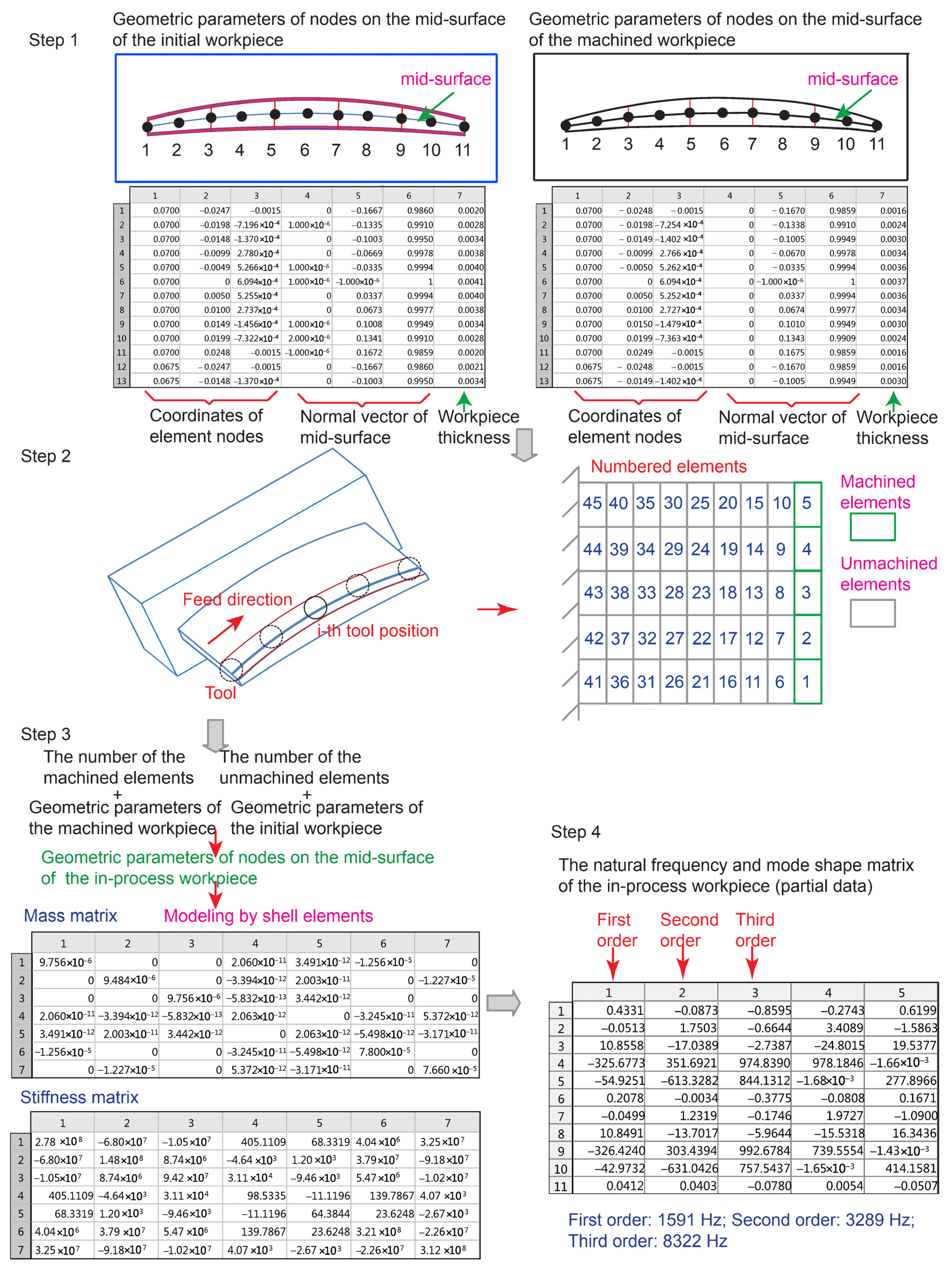
Use the same number of units to discretize the uncut workpiece and the machined workpiece, and use the method shown in Figure 3 to calculate the coordinates of the nodes on the arc surface of the discrete unit, the thickness of the blade corresponding to the nodes, and the normal vector of the mid-arc surface, and store them in the file.

(2)

Adopt the discrete method in step (1) to discretize the workpiece in the cutting process into the machined units and uncut units, and then number them.

(3)

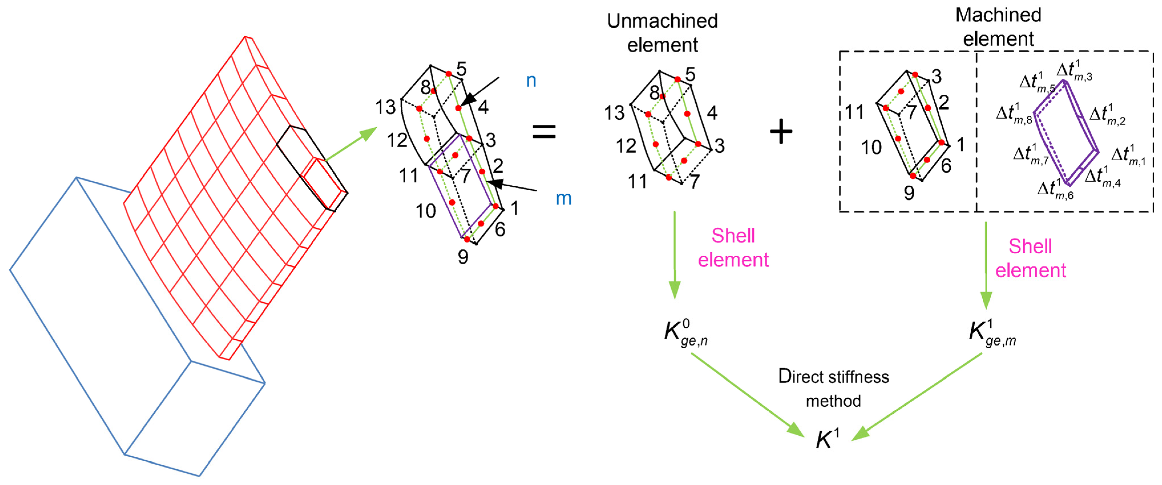
According to the discrete unit number of the workpiece in the cutting process in step (2), read the corresponding geometric parameters in step (1), establish a finite element model of the workpiece in the cutting process based on the shell unit, and calculate the stiffness matrix and mass matrix of the workpiece.

(4)

Using the calculated stiffness matrix and mass matrix of the workpiece, the nature frequency and mode shapes of the workpiece in the cutting process are calculated by solving the characteristic equations.

3. Neural Network-Based Prediction of Kinetic Parameters

Section 2 herein proposes a method for calculating the time-varying kinetic parameters for milling thin-walled parts based on shell cells, which only requires the geometrical parameters at the discrete cell nodes of the uncut and machined workpiece to calculate the workpiece kinetic parameters during the cutting process through finite element modeling. However, the abovementioned method consumes too much time to solve the characteristic equations for the finite element model of each cutting state. With the development of deep learning technology, neural networks have become widely used for cutting force predictions, tool life predictions, and predictions made in other fields. As demonstrated in Figure 6, neural networks offer a strong parallel computing capacity, which can predict the dynamic parameters of the workpiece in multiple cutting states at the same time, thereby significantly reducing the calculation time.

Herein, a three-layer neural network, as shown in Figure 6, is used for the thin-walled blade milling dynamic parameter prediction. Taking one single sample point as an example to describe the calculation process, the input quantity $t$ marks the thickness of the unit node and the output variable $f$ marks the first three orders of the nature frequency of the workpiece, which are denoted as follows:

$$\begin{array}{l}t={\left[\begin{array}{cccc}{t}_1& t_2& \cdots & t_n\end{array}\right]}^T\\ f={\left[\begin{array}{ccc}{f}_1& f_2& f_3\end{array}\right]}^T\end{array}$$

(21)

The ReLU function is used for the activation function, which is expressed as follows [31]:

$$R(x)=\max (0,x)$$

(22)

From the input $t$, the weight matrix $W^{[1]}$, the offset value $b^{[1]}$ of the first layer of the network, and the activation function calculation, we can obtain [32] as follows:

$$\begin{array}{l}{Z}^{[1]}=\left[\begin{array}{cccc}{w}_{1,1}^{[1]}& w_{1,2}^{[1]}& \cdots & w_{1,n}^{[1]}\\ w_{2,1}^{[1]}& w_{2,2}^{[1]}& \cdots & w_{2,n}^{[1]}\\ ⋮& ⋮& \ddots & ⋮\\ w_{m_1,1}^{[1]}& w_{m_1,2}^{[1]}& \cdots & w_{m_1,n}^{[1]}\end{array}\right]\left[\begin{array}{c}{t}_1\\ t_2\\ ⋮\\ t_n\end{array}\right]+b^{[1]}=W^{[1]}t+b^{[1]},\\ a^{[1]}=R(Z^{[1]})\end{array}$$

(23)

From the output $a^{[1]}$ of the first layer of the network, the weight matrix $W^{[2]}$, the offset value $b^{[2]}$ of the second layer of the network, and the activation function calculation, one can obtain the following:

$$\begin{array}{l}{Z}^{[2]}=\left[\begin{array}{cccc}{w}_{1,1}^{[2]}& w_{1,2}^{[2]}& \cdots & w_{1,m_1}^{[2]}\\ w_{2,1}^{[2]}& w_{2,2}^{[2]}& \cdots & w_{2,m_1}^{[2]}\\ ⋮& ⋮& \ddots & ⋮\\ w_{m_2,1}^{[2]}& w_{m_2,2}^{[2]}& \cdots & w_{m_2,m_1}^{[2]}\end{array}\right]\left[\begin{array}{c}{a}_1^{[1]}\\ a_2^{[1]}\\ ⋮\\ a_{m_1}^{[1]}\end{array}\right]+b^{[2]}=W^{[2]}{a}^{[1]}+b^{[2]},\\ a^{[2]}=R(Z^{[2]})\end{array}$$

(24)

From the output $a^{[2]}$ of the second layer of the network, the weight matrix $W^{[3]}$, and the offset value $b^{[3]}$ calculation of the third layer of the network, one can obtain the following:

$$f=\left[\begin{array}{c}{f}_1\\ f_2\\ f_3\end{array}\right]=\left[\begin{array}{cccc}{w}_{1,1}^{[3]}& w_{1,2}^{[3]}& \cdots & w_{1,m_2}^{[3]}\\ w_{2,1}^{[1]}& w_{2,2}^{[1]}& \cdots & w_{2,m_2}^{[1]}\\ w_{3,1}^{[1]}& w_{3,2}^{[1]}& \cdots & w_{3_1,m_2}^{[1]}\end{array}\right]\left[\begin{array}{c}{a}_1^{[2]}\\ a_2^{[2]}\\ ⋮\\ a_{m_2}^{[2]}\end{array}\right]+b^{[3]}=W^{[3]}{a}^{[2]}+b^{[3]}$$

(25)

The mean square error loss function between the predicted and nominal values of the nature frequency of the workpiece is established as follows:

$$L=\frac{1}{2}{‖f-\widehat{f}‖}^2$$

(26)

Thus, the prediction of the milling dynamic parameters for thin-walled parts is transformed into an optimization problem as follows:

$${\theta }^{*}=\underset{\theta }{\arg \min }L(\theta )$$

(27)

where parameter $\theta$ signifies the neural network weight matrix $W$ and the offset vector $b$, and the parameters $\theta$ are solved iteratively using the most rapid descent method.

The partial derivative of the loss function $L$ with respect to the weight matrix $W$ and the offset vector $b$ is expressed as follows:

$$\frac{\partial L}{\partial W^{[3]}}=(f-\widehat{f}){(a^{[2]})}^T$$

(28)

$$\frac{\partial L}{\partial W^{[2]}}={(W^{[3]})}^T(f-\widehat{f}){(a^{[1]})}^T$$

(29)

$$\frac{\partial L}{\partial W^{[1]}}={(W^{[2]})}^T{(W^{[3]})}^T(f-\widehat{f}){(t)}^T$$

(30)

$$\frac{\partial L}{\partial b^{[3]}}=f-\widehat{f}$$

(31)

$$\frac{\partial L}{\partial b^{[2]}}={(f-\widehat{f})}^T{W}^{[3]}$$

(32)

$$\frac{\partial L}{\partial b^{[1]}}={(f-\widehat{f})}^T{W}^{[3]}{W}^{[2]}$$

(33)

The parameters are iteratively updated using the most rapid descent method.

$$\begin{array}{l}W=W-\eta \frac{\partial L}{\partial W},\\ b=b-\eta \frac{\partial L}{\partial b},\end{array}$$

(34)

After the weight matrix $W$ and the offset vector $b$ are calculated, they are substituted into Equations (21)–(23), to calculate the nature frequency of the thin-walled part.

The whole frequency calculation steps are as follows.

(1)

Take the thickness of the unit node as the input quantity and the first three orders of the workpiece’s nature frequency as the output variable, and define the forward computation model with a fixed frequency, as shown in Equations (23)–(25).

(2)

Using the mean square deviation between the predicted values $f$ and nominal values $\widehat{f}$ of the workpiece’s nature frequency as the loss function, the prediction of the milling dynamic parameters of thin-walled parts is transformed into an optimization problem, as shown in Equation (27).

(3)

Iterative solution parameters, i.e., the neural network weight matrix $W$ and offset vectors $b$, are used through the most rapid descent method to calculate the nature frequency of the thin-walled parts.

4. Prediction and Validation of Milling Dynamic Parameters for Thin-Walled Parts

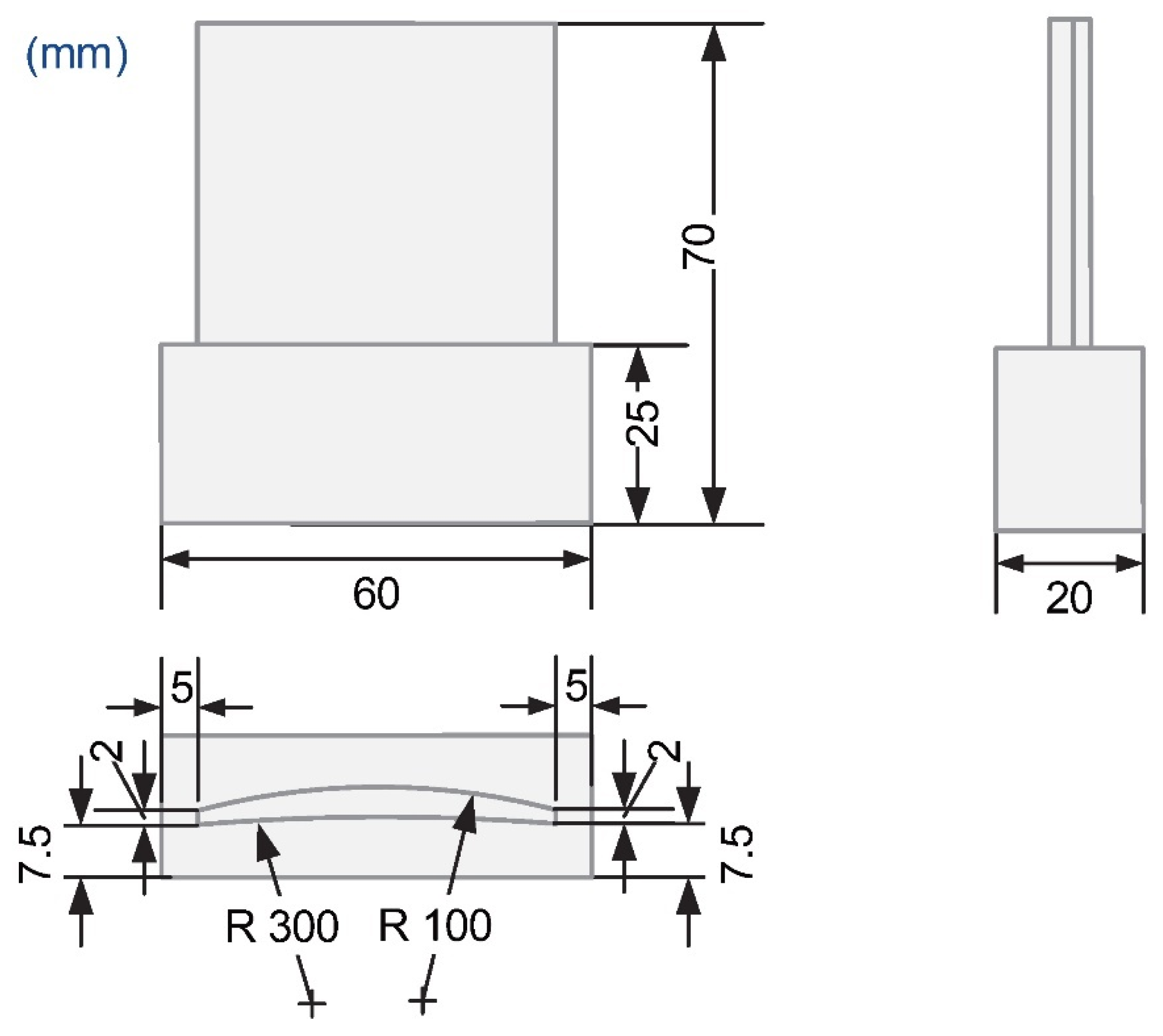
4.1. Finite Element Model Calculation and Test Verification

The titanium alloy TC4 test piece, with a density of 4500 kg/m³, a modulus of elasticity of 104 Gpa, and a Poisson’s ratio of 0.305, has its design dimensions shown in Figure 7.

After the mass and stiffness matrices of the FEM model have been obtained, the natural frequencies and the mode shapes of the workpiece can be calculated. However, degrees of freedom (DOF) of the FEM model affect the calculation speed of the characteristic equation. For reducing the number of DOF of the model on the premise of guaranteeing the calculation accuracy, a convergence analysis is performed. Meanwhile, the number of DOF of the model that is built by shell element and the model that is built by 3D cube element, which are used in the reference [15], are compared when the calculated natural frequencies achieve convergence. As the base of the blade is clamped by a fixture during machining, only the blade profile is modeled in the FEM modeling process in order to reduce the number of DOF of the model.

Matlab (R2014a) is used to build the FEM model of the blade based on the shell elements. To facilitate the following experimental verification, one element is set in the thickness direction, and five elements are set in the y-direction. The convergence of the natural frequencies is studied by increasing the number of elements (NOEs) in the x-direction from 6 to 9. Abaqus (6.14) is used to calculate the natural frequencies when the 3D cube elements with the type of C3D20R are used to model the blade. When the blade is meshed, two and five elements are set in the thickness direction and y-direction, respectively. The convergence of the natural frequencies is studied by increasing the NOEs in the x-direction from 4 to 8. As the high-order natural frequencies of the blade are difficult to be excited during machining, only the first three frequencies are studied in this paper. The convergence processes of the frequencies are shown in Figure 8. The values in parentheses show the variations the frequencies obtained by the present model and the previous model. It is supposed that when the variations are less than 0.1%, the natural frequencies reach convergence.

As shown in Figure 8a, when the NOES increases from 35 to 40, the maximum variation in the first three natural frequencies is 0.06%. Therefore, when the number of shell elements in the y-direction and x-direction are five and eight, respectively, the calculated frequencies reach convergence. At that point, the number of DOF of the shell model is 735, and when the clamped-free boundary conditions are imposed on the model, the number of DOF is 680. Meanwhile, Figure 8b shows that when the NOEs increases from 60 to 70, the maximum variation is 0.07%. At that point, the number of DOF of the cube model is 2916, and when the clamped-free boundary conditions are applied, the number of DOF is 2646. One can see the number of DOF of the FEM model established by the 3D cube elements is 3.89 times the size of the model established by the shell elements. This leads to about the nine times faster computation of the eigenvalues when the shell elements are used. When the value obtained by the 3D cube elements is regarded as a standard, the maximum error of the first three frequencies calculated by the shell elements is 0.38% and the average error is 0.237%. Therefore, under the premise of guaranteeing the calculation accuracy, the shell elements can reduce the number of DOF of the FEM model and thus reduce the time for calculating the dynamics of the blade. In the following point, the shell model is used to calculate the workpiece dynamics. Furthermore, one element is set in the thickness direction, five elements are set in the y-direction, and nine elements are set in the x-direction.

To verify the accuracy of the method proposed herein, the milling and modal testing of the thin-walled parts are performed on a five-axis machining center JD GR200-A10SH with a maximum spindle speed of 28,000 rpm, as shown in Figure 9. In the experiment, double-sided milling is used to simulate the actual machining condition of the blade. A four-tooth ball-end milling cutter with a diameter of 8 mm, a spindle speed of 3000 rpm, a feed rate of 300 mm/min, an axial depth of cut of 5 mm, and a radial depth of cut of 0.2 mm are used. The parameters of machining are shown in

Table 1. The parameters used in the test.

Spindle Speed (rpm)	Feed Rate (mm/min)	Axial Depth of Cut (mm)	Radial Depth of Cut (mm)
3000	300	5	0.2

.

The force hammer model is the Dytran Model 5800B (Marilla, CA, USA), the acceleration sensor model is Dytran 3224A1 (Marilla, CA, USA), and the data acquisition system is ECON-AVANT-8008 (Plymouth, MN, USA). This modal analysis software developed by Econ Company (North York, ON, USA) is used to extract the kinetic parameters of the workpiece. To ensure the validity of the test and shorten the test time, the modal test was conducted on the workpiece in six cutting stages. Step 0 represents the initial workpiece state when no cutting is performed and steps 1 to 5 each represents the material with a depth of 5 mm, 10 mm, 15 mm, 20 mm, and 25 mm along the direction of the removal. The moving force hammer test method with a fixed sensor is adopted herein, and the sticking position of the sensor and the hammering test points are shown in Figure 9, where point 3 is the response point of all the tests, namely the reference point. According to the structural characteristics of the blade, hammering is carried out at each test point along the direction of the blade.

The mode shapes extracted from the RFRs obtained through the tests and the FEM are compared, as shown in Figure 10, and the figures on the left show the results of the tests. It can be seen that the FEM results are consistent with the test results, and the mode shapes of modes 1 to 3 are the first bending mode, first torsional mode, and second bending mode, respectively.

After comparing and analyzing the nature frequency of the workpiece calculated using the finite element model with that of the workpiece obtained from the test during the milling process, the relative error is expressed as follows:

$${\eta }_1=\frac{f_{FEM}-f_{Test}}{f_{Test}}\times 100\%$$

(35)

where $f_{FEM}$ and $f_{Test}$ denote the frequencies of the workpiece obtained from the shell cell finite element model and the modal test, respectively. The calculated results are shown in

Table 2. Comparison of blade intrinsic frequencies (Hz) for the different cutting steps obtained from the shell cell finite element model and hammering test.

Steps	Modes	1	2	3
0	Tests	1535	3290	8152
	FEM	1574	3265	8293
	${\eta }_1$ (%)	(2.51)	(−0.76)	(1.72)
1	Tests	1552	3313	8094
	FEM	1591	3289	8233
	${\eta }_1$ (%)	(2.53)	(−0.73)	(1.71)
2	Tests	1551	3312	8101
	FEM	1604	3302	8299
	${\eta }_1$ (%)	(3.42)	(−0.32)	(2.45)
3	Tests	1548	3268	7972
	FEM	1611	3301	8244
	${\eta }_1$ (%)	(4.04)	(1.02)	(3.41)
4	Tests	1551	3239	7965
	FEM	1613	3286	8174
	${\eta }_1$ (%)	(4.01)	(1.44)	(2.62)
5	Tests	1550	3210	7867
	FEM	1609	3259	8112
	${\eta }_1$ (%)	(3.81)	(1.52)	(3.11)

, and the maximum errors of the results obtained from the shell cell finite element model are 2.51%, 2.53%, 3.42%, 4.04%, 4.01%, and 3.81%, respectively, compared with the test results. The experiment analysis shows that the shell finite element modeling method can effectively predict the time-varying dynamic parameters of the blade during the milling process.

4.2. Neural Network Model Predictive Analysis

For the thin-walled parts shown in Figure 7, the unit structure is discretized, and when the thickness $t$ of the nodes is taken as a fixed value, the first three orders of the nature frequency of the workpiece are calculated through the shell cell finite element model established herein, which is treated as a sample point. A total of 154 samples are obtained from the calculations herein of which 123 samples are taken as training samples. The model training learning rate is set to 0.01, the training data is disrupted, and the batch size is set to 30. The model is trained before the nature frequency of the workpiece is normalized to the first-order frequency because the nature frequency of the workpiece is higher relative to the thickness of the workpiece’s discrete unit node, and all the samples in the same batch will have the same predicted value when the model is being trained as per the example as follows:

$$f_N^1=\frac{f^1-f_{\min }^1}{f_{\max }^1-f_{\min }^1}$$

(36)

where $f^1$ represents the first-order frequency, $f_{\min }^1$ and $f_{\max }^1$ represent the minimum and maximum values of the first-order frequency of all the samples, respectively, and $f_N^1$ represents the normalized first-order frequency.

With the increase in the number of model training rounds, the convergence of the workpiece’s first three orders of nature frequency is displayed in Figure 11, where one can see that the predicted value reaches convergence when the epoch = 300, and the epoch = 300 is adopted herein for calculation. The comparison of the nature frequency of the workpiece at various cutting stages, which is calculated using the neural network model and the shell cell finite element model, is shown in

Table 3. Comparison of blade intrinsic frequencies (Hz) during the cutting calculated using the neural network model (NN) and shell cell finite element model (FEM).

State	Modes	1	2	3	State	Modes	1	2	3
1	FEM	1536	3002	7538	7	FEM	1589	3032	7370
	NN	1534	3004.5	7545.1		NN	1584	3037.1	7368.6
	$\eta$ (%)	(−0.12)	(0.082)	(0.095)		$\eta$ (%)	(−0.31)	(0.168)	(−0.019)
2	FEM	1512	2965	7523	8	FEM	1557	2957	7322
	NN	1510	2967	7526.4		NN	1556	2964.6	7333.7
	$\eta$ (%)	(−0.11)	(0.067)	(0.046)		$\eta$ (%)	(−0.03)	(0.255)	(0.16)
3	FEM	1553	3099	7806	9	FEM	1505	2881	7289
	NN	1549	3098	7821.4		NN	1509	2889.6	7296.3
	$\eta$ (%)	(−0.29)	(−0.001)	(0.197)		$\eta$ (%)	(0.25)	(0.298)	(0.099)
4	FEM	1581	3131	7748	10	FEM	1496	2954	7487
	NN	1576	3131.9	7766.3		NN	1500	2960.9	7517.1
	$\eta$ (%)	(−0.30)	(0.0027)	(0.236)		$\eta$ (%)	(0.28)	(0.233)	(0.401)
5	FEM	1598	3131	7624	11	FEM	1511	2970	7459
	NN	1593	3132.5	7628.7		NN	1514	2977.3	7489.5
	$\eta$ (%)	(−0.31)	(0.047)	(0.062)		$\eta$ (%)	(0.20)	(0.247)	(0.409)
6	FEM	1602	3095	7479	12	FEM	1519	2969	7400
	NN	1598	3094.3	7486.3		NN	1522	2977.6	7420.7
	$\eta$ (%)	(−0.23)	(−0.023)	(0.098)		$\eta$ (%)	(0.23)	(0.291)	(0.28)

. When the results of the shell cell finite element model are treated as the benchmark, the maximum error of the first three orders of nature frequency calculated using the three-layer neural network model reaches 0.409%. Therefore, the kinetic parameters of the workpiece during the cutting process can be efficiently predicted by training the three-layer neural network model.

Next, the computational efficiency of the shell cell finite element model is compared with the three-layer neural network model. The stiffness matrix and mass matrix of the shell unit finite element model of the thin-walled parts herein have 765 degrees of freedom, and the characteristic equation is solved by using Matlab software to calculate the nature frequency of the workpiece. For one sample, the solution time reaches 11.771 s. When epoch = 300 and batch size = 30, the CPU is used for computation, and the training time of the three-layer neural network model is shown in Figure 12a, which is about 9 s. After obtaining the neural network computational model from the training data, the kinetic parameters of the workpiece at different cutting stages can be batch-computed using the model. The time spent predicting the kinetic parameters of the workpiece through the neural network model is shown in Figure 12b. The loading time of the neural network model and its input data loading time amount to 1.6611 s. The prediction time is only 0.00315 s for the 150-numbered samples. The model training time is only 4 s when the GPU is used for the computation.

The modal testing results showed that the maximum prediction error of the FEM was 4.04%. In comparison with the calculations using the FEM, the neural network model exhibited a maximum prediction error of 0.409%, thereby suggesting that the neural network model’s maximum prediction error is approximately 4% when compared with the modal testing results. The abovementioned analysis shows that compared with the shell cell finite element model, the computation efficiency can be significantly improved by utilizing the batch computation function of the neural network while guaranteeing prediction accuracy.

5. Conclusions

In this paper, the neural network model is introduced into the prediction of the dynamic parameters of thin-walled parts to achieve the real-time and rapid prediction of workpiece dynamics during the milling of thin-walled parts. Firstly, the FEM based on shell elements was built. After the node coordinates, workpiece thickness, and normal vector of the intermediate surface of the initial workpiece and the machined workpiece were obtained, the established shell FEM was used to calculate the time-varying dynamic parameters of the workpiece during the milling process. To improve the computational efficiency, a three-layer neural network model was constructed to predict the time-varying dynamic parameters for milling the thin-walled parts. Then, the dataset obtained using the shell FEM was used as the training samples to train the neural network model. Finally, the effectiveness of the model was verified through modal testing experiments. The following conclusions can be drawn.

(1)

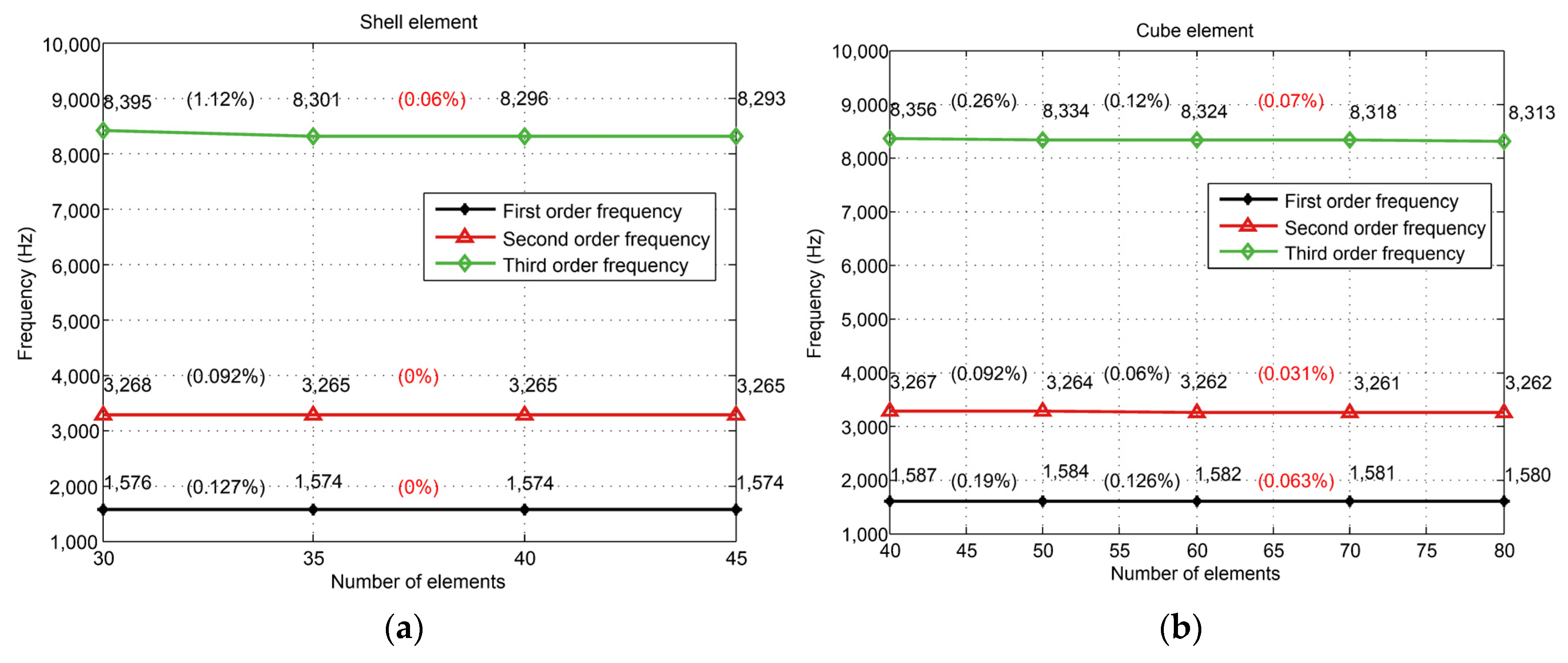
The proposed method only needs to mesh the initial workpiece and the machined workpiece once, and it only needs to calculate the geometric parameters of the initial workpiece and the machined workpiece. It does not need to re-mesh the thin-walled parts at each cutting position and to repeatedly calculate the geometric parameters of the workpiece during the cutting process. Meanwhile, in comparison with the three-dimensional cube elements, the shell elements can reduce the number of degrees of freedom of the FEM model by 74%, which leads to about nine times faster computation of the characteristic equation.

(2)

Modal test results show that the maximum prediction error of the workpiece nature frequency of the built shell FEM is about 4%.

(3)

Compared with the calculation results of the FEM, the maximum prediction error of the neural network model is 0.409%. It can be inferred that compared with the modal test results, the maximum prediction error of the neural network model is about 4%.

(4)

When the training samples are 132, the epoch is 300, the batch size is 30, and the CPU is used for calculation, the training time is about 9 s. When using the model to batch-calculate the dynamic parameters of a thin-wall part at different cutting stages, the loading time of the neural network model and the model input data is about 1.6611 s. When the number of predicted cutting states is 150, the prediction time is only 0.00315 s. Therefore, the three-layer neural network model can highly improve calculation efficiency while ensuring calculation accuracy.

Meanwhile, the present study has certain limitations. As compared with modal testing, the prediction error of the FEM is about 4%, and this results in an approximate 4% prediction error in the neural network model. In the future, a dataset of workpiece thickness and natural frequencies will be constructed based on modal testing experiments. Then, the prediction accuracy of the neural network model will be enhanced.

References

1. Zhao, G.L.; Zhao, B.; Ding, W.F.; Xin, L.J.; Nian, Z.W.; Peng, J.H.; He, N.; Xu, J.H. Nontraditional energy-assisted mechanical machining of difficult-to-cut materials and components in aerospace community: A comparative analysis. Int. J. Extreme Manufacturing 2023, 6, 022007. [Google Scholar] [CrossRef]
2. Bravo, U.; Altuzarra, O.; De Lacalle, L.N.L.; Sánchez, J.A.; Campa, F.J. Stability limits of milling considering the flexibility of the workpiece and the machine. Int. J. Mach. Tools Manuf. 2005, 45, 1669–1680. [Google Scholar]
3. Seguy, S.; Campa, F.J.; De Lacalle, L.N.L.; Arnaud, L.; Dessein, G.; Aramendi, G. Toolpath dependent stability lobes for the milling of thin-walled parts. Int. J. Mach. Mach. Mater. 2008, 4, 377. [Google Scholar] [CrossRef]
4. Arnaud, L.; Gonzalo, O.; Seguy, S.; Jauregi, H.; Peigné, G. Simulation of low rigidity part machining applied to thin-walled structures. Int. J. Adv. Manuf. Technol. 2011, 54, 479–488. [Google Scholar] [CrossRef]
5. Thevenot, V.; Arnaud, L.; Dessein, G.; Cazenave-Larrocheet, G. Influence of material removal on the dynamic behavior of thin-walled structures in peripheral milling. Mach. Sci. Technol. 2006, 10, 275–287. [Google Scholar] [CrossRef]
6. Song, Q.H.; Ai, X.; Tang, W.X. Prediction of simultaneous dynamic stability limit of time–variable parameters system in thin-walled workpiece high-speed milling processes. Int. J. Adv. Manuf. Technol. 2011, 55, 883–889. [Google Scholar] [CrossRef]
7. Meshreki, M.; Attia, H.; Kövecses, J. Development of a new model for the varying dynamics of flexible pocket-structures during machining. J. Manuf. Sci. Eng. Am. Soc. Mech. Eng. 2011, 133, 41002. [Google Scholar] [CrossRef]
8. Song, Q.H.; Liu, Z.Q.; Wan, Y.; Ju, G.G.; Shi, J.H. Application of Sherman-Morrison-Woodbury formulas in instantaneous dynamic of peripheral milling for thin-walled component. Int. J. Mech. Sci. 2015, 96, 79–90. [Google Scholar] [CrossRef]
9. Song, Q.H.; Shi, J.H.; Liu, Z.Q.; Wan, Y. A time-space discretization method in milling stability prediction of thin-walled component. Int. J. Adv. Manuf. Technol. 2017, 89, 2675–2689. [Google Scholar] [CrossRef]
10. Ahmadi, K. Finite strip modeling of the varying dynamics of thin-walled pocket structures during machining. Int. J. Adv. Manuf. Technol. 2017, 89, 2691–2699. [Google Scholar] [CrossRef]
11. Tuysuz, O.; Altintas, Y. Frequency domain updating of thin-walled workpiece dynamics using reduced order substructuring method in machining. J. Manuf. Sci. Eng. Am. Soc. Mech. Eng. 2017, 139, 71013. [Google Scholar] [CrossRef]
12. Yang, Y.; Zhang, W.H.; Ma, Y.C.; Wan, M. Chatter prediction for the peripheral milling of thin-walled workpiece with curved surfaces. Int. J. Mach. Tools Manuf. 2016, 109, 36–48. [Google Scholar] [CrossRef]
13. Yang, Y.; Zhang, W.H.; Ma, Y.C.; Wan, M.; Dang, X.B. An efficient decomposition-condensation method for chatter prediction in milling large-scale thin-walled structures. Mech. Syst. Signal Process. 2019, 121, 58–76. [Google Scholar] [CrossRef]
14. Dang, X.B.; Wan, M.; Yang, Y.; Zhang, W.H. Efficient prediction of varying dynamic characteristics in thin-wall milling using freedom and mode reduction methods. Int. J. Mech. Sci. 2019, 150, 202–216. [Google Scholar] [CrossRef]
15. Budak, E.; Tun, L.T.; Alan, S.; Nevzat-Özgüvenet, H. Prediction of workpiece dynamics and its effects on chatter stability in milling. CIRP Ann. 2012, 61, 339–342. [Google Scholar] [CrossRef]
16. Zhang, X.; Zhu, L.; Ding, H. Matrix perturbation method for predicting dynamic modal shapes of the workpiece in high-speed machining. Proc. Inst. Mech. Eng. Part B J. Eng. Manuf. 2010, 224, 177–183. [Google Scholar] [CrossRef]
17. Luo, M.; Zhang, D.H.; Wu, B.H.; Tang, M. Modeling and analysis effects of material removal on machining dynamics in milling of thin-walled workpiece. Adv. Mater. Res. 2011, 223, 671–678. [Google Scholar] [CrossRef]
18. Tian, W.J.; Ren, J.X.; Zhou, J.H.; Wang, D.Z. Dynamic modal prediction and experimental study of thin-walled workpiece removal based on perturbation method. Int. J. Adv. Manuf. Technol. 2018, 94, 2099–2113. [Google Scholar] [CrossRef]
19. Ju, G.G. Research on Instability Characteristics of Thin-walled Parts with Complex Curved Surface and Variable Thickness during Multi-Axis Milling. Master’s Thesis, Shandong University, Jinan, China, 2016. [Google Scholar]
20. Tuysuz, O.; Altintas, Y. Time-domain modeling of varying dynamic characteristics in thin-wall machining using perturbation and reduced-order substructuring methods. J. Manuf. Sci. Eng. 2018, 140, 011015. [Google Scholar] [CrossRef]
21. Liu, Y.L. Analysis of Milling Dynamics and Chatter Detection and Control Methods for Thin-Walled Workpiece. Ph.D. Thesis, Northwestern Polytechnical University, Xi’an, China, 2017. [Google Scholar]
22. Kim, D.H.; Kim, T.Y.; Wang, X.L.; Kim, M.; Quan, Y.J.; Oh, J.W.; Min, S.H.; Kim, H.J.; Bhandari, B.; Yang, I.; et al. Smart Machining Process Using Machine Learning: A Review and Perspective on Machining Industry. Int. J. Precis. Eng. Manuf.-Green Technol. 2018, 5, 555–568. [Google Scholar] [CrossRef]
23. Yeganefar, A.; Niknam, S.A.; Asadi, R. The use of support vector machine, neural network, and regression analysis to predict and optimize surface roughness and cutting forces in milling. Int. J. Adv. Manuf. Technol. 2019, 105, 951–965. [Google Scholar] [CrossRef]
24. Pavlenko, I.; Saga, M.; Kuric, I.; Kotliar, A.; Basova, Y.; Trojanowska, J.; Ivanov, V. Parameter identification of cutting forces in crankshaft grinding using artificial neural networks. Materials 2020, 13, 5357. [Google Scholar] [CrossRef]
25. SK, T.; Shankar, S.; T, M.; K, D. Tool wear prediction in hard turning of EN8 steel using cutting force and surface roughness with artificial neural network. Proc. Inst. Mech. Eng. Part C J. Mech. Eng. Sci. 2020, 234, 329–342. [Google Scholar] [CrossRef]
26. Vasanth, X.A.; Paul, P.S.; Varadarajan, A.S. A neural network model to predict surface roughness during turning of hardened SS410 steel. Int. J. Syst. Assur. Eng. Manag. 2020, 11, 704–715. [Google Scholar] [CrossRef]
27. Wang, J.; Zou, B.; Liu, M.; Li, Y.; Ding, H.; Xue, K. Milling force prediction model based on transfer learning and neural network. J. Intell. Manuf. 2021, 32, 947–956. [Google Scholar] [CrossRef]
28. Heitz, T.; He, N.; Ait-Mlouk, A.; Bachrathy, D.; Chen, N.; Zhao, G.; Li, L. Investigation on eXtreme Gradient Boosting for cutting force prediction in milling. J. Intell. Manuf. 2023. [Google Scholar] [CrossRef]
29. Zhu, B.F. ; The Finite Element Method Theory and Applications; China Institute of Water Resources and Hydropower Research: Beijing, China, 2018. [Google Scholar]
30. Logan, D.L. A First Course in the Finite Element Method; Cengage Learning: Boston, MA, USA, 2011. [Google Scholar]
31. Agarap, A.F. Deep learning using rectified linear units (relu). arXiv 2018, arXiv:1803.08375. [Google Scholar]
32. Goodfellow, I.; Bengio, Y.; Courville, A. Deep Learning; MIT Press: Cambridge, MA, USA, 2016. [Google Scholar]
Figure 1. Simplification and discretization of the blade process model.
Jmmp 08 00043 g001
Figure 2. The eight-node thick shell cell.
Jmmp 08 00043 g002
Figure 3. Flow of the workpiece stiffness matrix calculation during the thin-walled blade cutting process.
Jmmp 08 00043 g003
Figure 4. Flow of calculating the geometrical parameters of the discrete unit nodes on the curved surfaces of thin-walled blades.
Jmmp 08 00043 g004
Figure 5. The process of calculating the parameters of the workpiece dynamics during the cutting process.
Jmmp 08 00043 g005
Figure 6. Neural network structure diagram.
Jmmp 08 00043 g006
Figure 7. Structural design dimensions of thin-walled parts.
Jmmp 08 00043 g007
Figure 8. Convergence process of the natural frequencies (Hz) (a) obtained by shell element and (b) obtained by cube element.
Jmmp 08 00043 g008
Figure 9. Milling modal test experiment for the thin-walled parts of a blade.
Jmmp 08 00043 g009
Figure 10. Mode shapes obtained through tests and the FEM as follows: (a) mode 1, (b) mode 2, and (c) mode 3.
Jmmp 08 00043 g010aJmmp 08 00043 g010b
Figure 11. Convergence analysis of the neural network model’s predictive values. (a) First-order nature frequency, (b) second-order nature frequency, (c) third-order nature frequency.
Jmmp 08 00043 g011
Figure 12. Design neural network model training and prediction time. (a) Neural network model training time, (b) neural network batch prediction time for the milling dynamic parameters of the thin-walled parts.
Jmmp 08 00043 g012