Article

Implications from Legacy Device Environments on the Conceptional Design of Machine Learning Models in Manufacturing

1
Institute of Digital Engineering, Technical University of Applied Sciences Wuerzburg-Schweinfurt, Ignaz-Schön-Strasse 11, 97421 Schweinfurt, Germany
2
Cybus GmbH, Osterstraße 124, 20255 Hamburg, Germany
*
Author to whom correspondence should be addressed.
J. Manuf. Mater. Process. 2024, 8(1), 15; https://doi.org/10.3390/jmmp8010015
Submission received: 6 December 2023 / Revised: 7 January 2024 / Accepted: 15 January 2024 / Published: 17 January 2024

Abstract

:
While new production areas (greenfields) have state-of-the-art technologies for implementing digitalization, existing production areas (brownfields) and devices must first be upgraded with technologies before digitalization can be implemented. The aim of this research work is to use a case study to identify the differences in the implementation of machine learning (ML) projects in brownfields and greenfields. For this purpose, an ML application for the detection of changeover times on milling machines is implemented and analyzed in the brownfield and greenfield scenarios as well as a combined scenario. Particular attention is paid to the selection of sensors and features. It was found that the abundant availability of features in the greenfield scenario poses pitfalls when creating ML projects if the underlying sensors cannot be checked for their suitability. For the changeover detector use case, the best model quality was achieved for the combined scenario, followed by the greenfield scenario.

1. Introduction

Digitization can support manufacturing companies in their efforts to improve efficiency in their processes. The research project Optimization of Processes and Machine Tools through Provision, Analysis and Target/Actual Comparison of Production Data (OBerA) was founded with the aim of supporting companies from Bavaria in the application of digitization techniques and investigating the possibilities and challenges of the approaches. The OBerA project consortium consisted of five production-oriented companies from the small and medium-sized enterprise (SME) sector [1], Siemens as the technology partner, and the Technical University of Applied Sciences Würzburg-Schweinfurt as the research partner.
Throughout the research project, digitization techniques were implemented in collaboration with the project partners. Based on these techniques, various optimization projects were carried out, employing machine learning (ML) concepts in machine changeover, production planning, tool management, and factory automation. Significant variations in the results were noted between older machine environments (brownfield) and areas featuring modern infrastructure (greenfield). Therefore, the question arose as to whether different procedures are required for optimization projects with ML or whether existing procedures need to be adapted.
In Section 1.1, first, the terms greenfield and brownfield are clarified and characterized in the field of ML projects based on current research articles. The importance of data acquisition and, in particular, sensor and feature selection is then emphasized. The differences between a greenfield and a brownfield approach are elaborated, which have not yet been addressed in current research work. A research gap and research questions are derived from these findings. In Section 1.2, the research approach based on a use case evaluation is described. In Section 1.3, the structure of the article is presented.

1.1. Problem Statement

In the transition to a smart factory, the integration of sensors and data processing becomes crucial for both logistical and production processes. Usually, the planning of factories or production lines involves incorporating current technology from the ground up. This approach is called the greenfield approach. According to [2], greenfield planning can be conducted on “a new production site or a new production system within an existing site”.
While greenfield sites are emerging from a stable economic situation, brownfield environments are often economically regarded as marginally viable or even non-viable sites. Economically, these sites cannot compete with greenfield sites [3].
A legacy system, as part of a brownfield environment, contains machines from different manufacturing dates with different technology levels. Process control is conducted manually, including “observing, sensing, estimating, and adjusting the machine parameters” [4].
In terms of digitization, several challenges exist for upgrading brownfield environments to the comparable capabilities of greenfield environments. The term retrofitting is often used to describe the upgrade of brownfield environments with Industry 4.0 capabilities [5], including “the hardware of machinery and the production method, operator, and management” [4]. In particular, machines from brownfield sites need to be equipped with sensors and connectivity [6]. For up-to-date machines in greenfield sites, machine states are made available for ML applications via software architectures that are typically manufacturer-dependent. In this context, selecting features from the machine’s almost inexhaustible choice of features presents a challenge in creating ML models. But, despite the advantages of greenfield sites, it is technically or economically not always possible to replace brownfield machinery [5].
Brownfield machines, on the other hand, lack sensors and connectivity. Here, the selection, application, and connection of sensors are challenges. The number of features is more limited in comparison to the greenfield case. Often, sensors are specifically chosen according to operational needs or the technical optimization target related to process or quality parameters [4]. Integrating many different sensor types also depends on the available budget for sensors and the efforts to integrate them into a common data platform [7].
The different availability of features in brownfield and greenfield scenarios has consequences for the creation of ML models. In the case of the brownfield scenario, the quality of the model created depends on selecting a suitable set of sensors. In the case of the greenfield scenario, the quality of the created model depends on a so-called feature selection process.
While feature selection is a common task in ML [8], selecting suitable sensors should also be supported methodically. In [9], from expert interviews, the authors state that feature selection in ML software projects is focused on “accessibility, accuracy, authoritativeness, freshness, latency, structuredness, ontological typing, connectedness, and semantic joinability”. The selection of sensors, which has to be conducted before the accessibility of data can be considered, was not mentioned by the respondents. Conclusively, the authors declare that “engineers have to find … data for use in model training and tuning”, though they do not provide specific directions on how this search shall be conducted. The lack of a methodological approach for practitioners of ML projects can be considered a research gap. In [10], the authors point out that approaches for the development of technical systems for greenfield and brownfield situations have different characteristics. A methodological approach, therefore, should take greenfield and brownfield characteristics into account. The corresponding first research question for this article is “Which methods are suitable for brownfields (and, subsequently, greenfields) to support the sensor selection process for ML projects?”
In their article about data science projects on industrial data in brownfields [11], the authors point out the importance of thorough planning of data acquisition. They also emphasize that findings from greenfield approaches need to be checked for generalizability before applying them to brownfield approaches, and vice versa. Overall, if the initial data acquisition approach between greenfield and brownfield optimization approaches differs, the following question arises: what will be the impact on the result of the optimization? The second research question, therefore, examines the effect of a methodically supported sensor selection process on the quality of the ML model created: “What differences can be seen between the performance metrics of ML models from a brownfield, greenfield, and a combined approach?”

1.2. Research Approach

The first research question aims to identify existing methods for sensor selection and analyze these methods for their suitability for use in ML projects in brownfield and greenfield environments. Existing methods are often used as part of procedures. Overall, the research question has an exploratory objective. The available data describe the methods and procedures and can, therefore, be described as qualitative. Due to the exploratory objective and the qualitative data, case study research is used as a research strategy ([12], p. 15).
In order to broaden this empirical research approach, information from three different scenarios is considered (data source triangulation, [12], p. 16). The three scenarios are related to a greenfield, brownfield, and mixed environment (here: combined). For all these scenarios, the exemplary use case of changeover detection based on manufacturing data is used to create ML models. On the one hand, this seems to be a specific application, but on the other hand, many different production machines are usually set up to change from one variant to another (changeover); previous research work has shown that the detection of changeovers requires many different uses of data sources [13]. This specific use case of changeover is implemented for the three scenarios for five-axis milling, which is a general and widely used manufacturing technology.
Sensor selection is part of the implementation process for ML models. The exemplary procedure proposed by [4] for a holistic digitization concept is applied here:
  • Sensors (and actuators) for process interaction;
  • Connectivity for communication and automation;
  • Data management for data accumulation and abstraction;
  • Operational integration for business decisions.
Even though the focus of the research work is on the sensor selection step, all steps (but not the actuator interaction) are carried out in this article. At the end of the creation of the ML model, the model quality is also included in the discussion as additional information with which to evaluate the suitability for operational integration. Strictly speaking, the model metric as a measure of the model quality is a quantitative characteristic that will be taken into account to discuss the overall success of the methodology.
The applied ML algorithms are from the family of supervised learning algorithms that rely on labeled data as ground truth [9]. Methods of unsupervised learning, reinforcement learning, or others are not considered in this article [14,15,16].

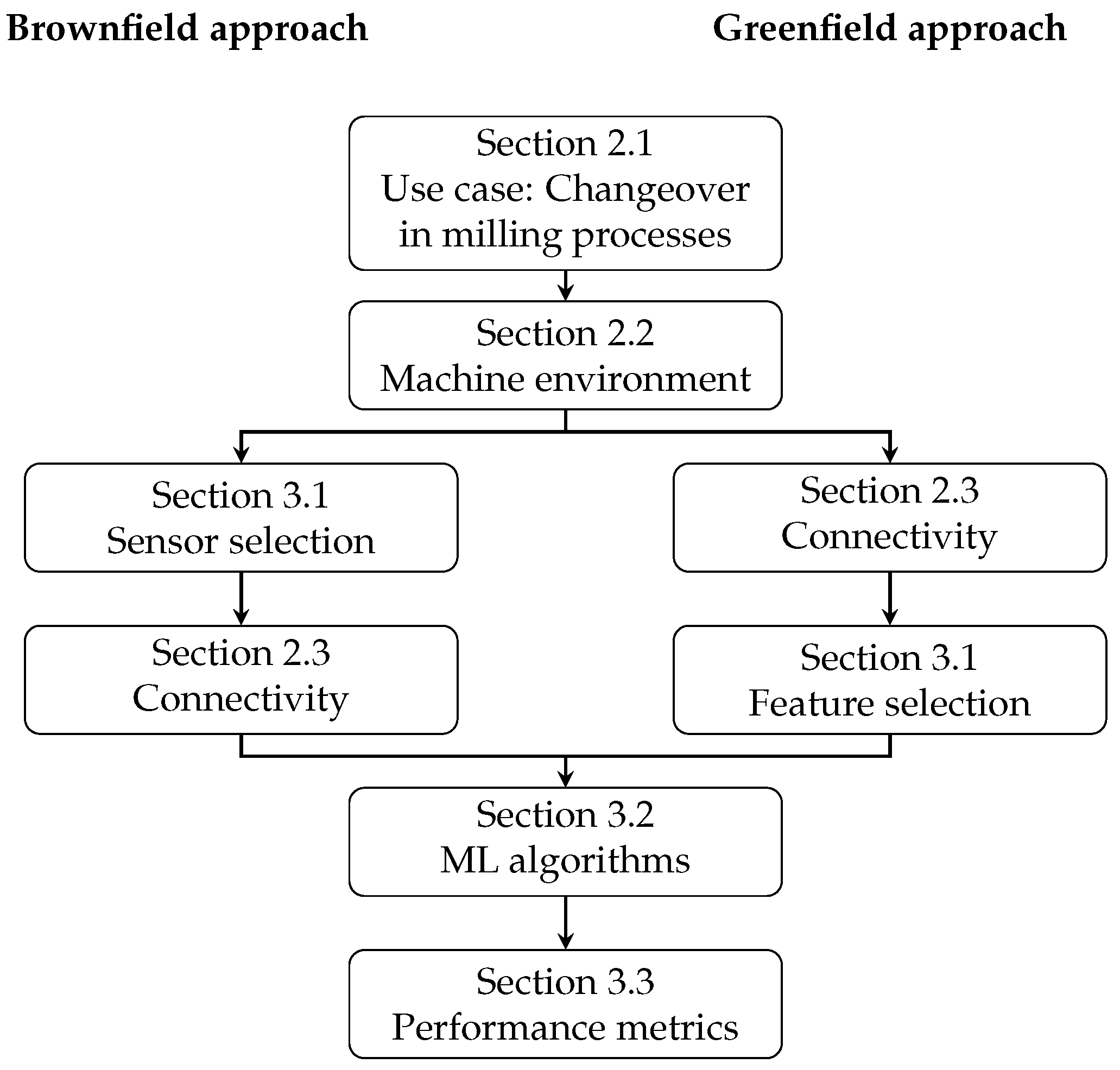
1.3. Article Structure

The article is structured in a classical way, starting with a materials section (Section 2). Section 2.1 explains the use case of a changeover detector for manufacturing machines. The very heterogeneous machine environment of the project consortium used to realize this use case is analyzed, the most frequent numerical control (NC) manufacturers are roughly portrayed, and the specifically used machines are presented (Section 2.2). Section 2.3 describes the connectivity setups for the different scenarios (brownfield, greenfield, and combined approach).
Then, the supporting methods are presented in the methods section (Section 3). Here, the focus is set on feature and sensor selection methods for the different approaches (Section 3.1). The selected ML algorithms to model the use case are explained (Section 3.2), as are the performance metrics used for the ML models (Section 3.3).
In the results section (Section 4), the implementation of the changeover detector is analyzed for the different scenarios as well as the performance metrics for the selected ML algorithms. The results are discussed in Section 5.
Finally, conclusions are derived in Section 6.1, and directions for further research are elaborated (Section 6.2).

2. Materials

The materials section introduces the use case of a changeover detector for manufacturing machines (Section 2.1) and explains the machine environment of the project consortium (Section 2.2). Moreover, an analysis of the most frequent numerical control (NC) manufacturers used in the consortium is presented. Section 2.3 explains the resulting connectivity challenges for the brownfield, greenfield, and combined approaches.

2.1. Use Case Description

In prior research, a machine learning (ML) approach for milling machines was developed to distinguish between changeover and production phases. Changeover refers to the period during which a production machine is prepared for the next product variant. This changeover detector uses data from external sensors and the machine’s operational states to evaluate whether a production machine is in changeover or production mode. The ML task involves classifying the current sensor readings and machine status information into two distinct manufacturing phases (No. 1, “Changeover”: changeover, including intermittent idle time; No. 2, “Production”: the production phase). Although the original ML approach incorporated additional changeover phases, this article focuses on comparing the different approaches within these two phases.
Based on the changeover detector use case, three scenarios were defined to evaluate the different effects of creating ML models in brownfield, greenfield, and mixed environments (here: combined):
For the brownfield scenario, the ML model was based on a setup of external sensors, which were applied to an existing antiquated milling machine (DMG 100 U duoBLOCK, see also Section 2.2.4). These sensors were not connected to the numerical control (NC) of the machines (“NC-external”). This brownfield approach did not require an up-to-date NC to connect specific sensors (see Table 1, left). However, as was shown in [17], all the different sensors had to be connected using their specific hardware interface (i.e., IO-Link, digital I/O, internal programmable logic controller (PLC)) and the data needed to be collected (over message queuing telemetry transport (MQTT)) and aggregated in a common structured query language (SQL) database.
For the combined approach, the external sensor setup was further enhanced by data that were available directly from the NC (see Table 1, middle). Data were collected from internal sensors, which were made available externally by the NC or were the internal statuses or computed values of the NC (“NC-provided”). This approach was defined as the combined approach (see Table 1, middle). The additional NC-provided sensors aggravated the sensor selection problem, which was identified for the brownfield approach. Furthermore, the same information can be available in different variables in an NC. This underlined the necessity of feature selection, which is a common activity of ML projects ([18], p. 27). When using information directly from an NC, there are proprietary interfaces provided by the NC manufacturers that have specific architectures (see Section 2.2). In order to connect new sensors to the NC and enable them in software interfaces, maintenance personnel need to be trained and available. For example, a door switch is already connected to the NC, but the internal variable of the door switch has to be identified in the wiring plans and made available for the data interface by a maintenance technician. This article shows that, aside from these necessary efforts, the quality of the model can be improved by additional NC-provided data (see Section 4).
The greenfield approach (see Table 1, right) relies solely on NC-provided variables and sensors. In comparison to the brownfield and the combined approach, the greenfield approach offers standardized access to the NC (e.g., switch cabinet techniques and standardized NC programming) and reduces the number of sensor interfaces that have to be connected.

2.2. Machine Environments

The machine control landscape in the OBerA consortium is very heterogeneous. Figure 1 shows an overview of the different machine controls that exist in the different companies of the consortium. The controls from Siemens, FANUC, and HEIDENHAIN are the most frequently used in the consortium. However, it needs to be pointed out that the number of Siemens controls exceeds that of the other manufacturers, as one of the companies of the consortium is a Siemens production site.
Every NC manufacturer has its own interface approach to making machine data available. The different concepts of the manufacturers (Siemens, FANUC, and HEIDENHAIN) for retrieving NC data are described in the following sections. A new approach called universal machine technology interface (umati) provides a framework for standardized communication. It is based on the Open Platform Communications Unified Architecture (OPC UA) protocol but is still under development and not commonly available [19]. Therefore, it is not considered in this article.
Table 2 shows exemplary reported usages for machine control interfaces from Siemens, FANUC, and HEIDENHAIN in scientific research articles. For all NC manufacturers, the machining operation for milling is reported. For FANUC and Siemens, turning is also mentioned in some articles. Additionally, drilling and laser cutting use cases were reported for Siemens.

2.2.1. Siemens

Siemens mainly uses its platform (Mindsphere) to collect and store NC data. It supports various communication protocols, such as MQTT, OPC UA, FANUC FOCAS, Modbus, etc. [31]. Additional hardware can be used to transfer data to the Mindsphere, and existing hardware can be connected through a supplementary software library [32]. Siemens distinguishes between high- and low-frequency data. The SINUMERIK Edge concept allows up to 100 high-frequency variables (1 kHz), which are taken directly from the NC kernel with data from interpolation or position control. Low-frequency data can be distributed by the BTSS concept that gives access, e.g., to PLC, static, or system NC variables.

2.2.2. FANUC

FANUC has its own software solution to collect data from machines, robots, and other devices called MT-LINKi. It can connect to FANUC machines by using the FOCAS library, machines from other manufacturers, PLCs, and sensors, as long as they are in a network supporting OPC UA or MTConnect [33]. By using the FOCAS library, “own functions” can be developed [34]. The FANUC OPC server can be used to convert the communication protocols between OPC and FOCAS [35].

2.2.3. HEIDENHAIN

In order to obtain data from HEIDENHAIN machines, the HEIDENHAIN DNC interface can be used. These data can be exchanged with numerous systems like enterprise resource planning (ERP), CAD, or simulation software [36]. HEIDENHAIN has its own platform for collecting, interpreting, and visualizing machine data. It can collect data from its own distributed numerical control (DNC), OPC UA, MTConnect, and Modbus/TCP [37]. Problems can arise if the NC is too old to communicate with the interface. Machine controls manufactured before the year 2006 cannot communicate via the HEIDENHAIN DNC [38].

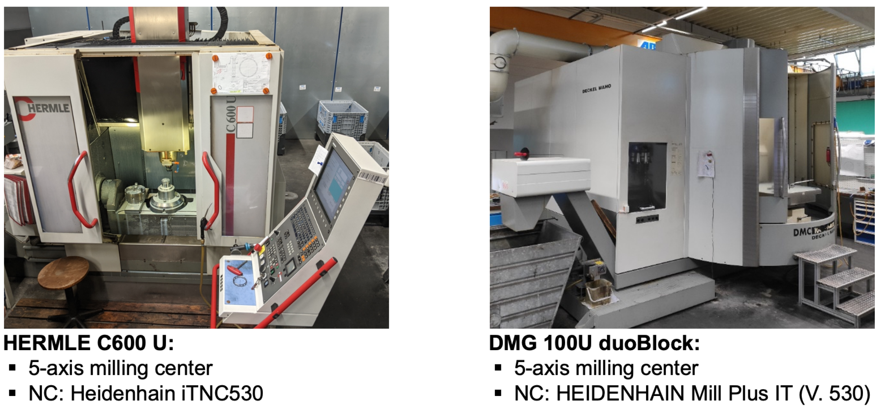
2.2.4. Used Machine Tools
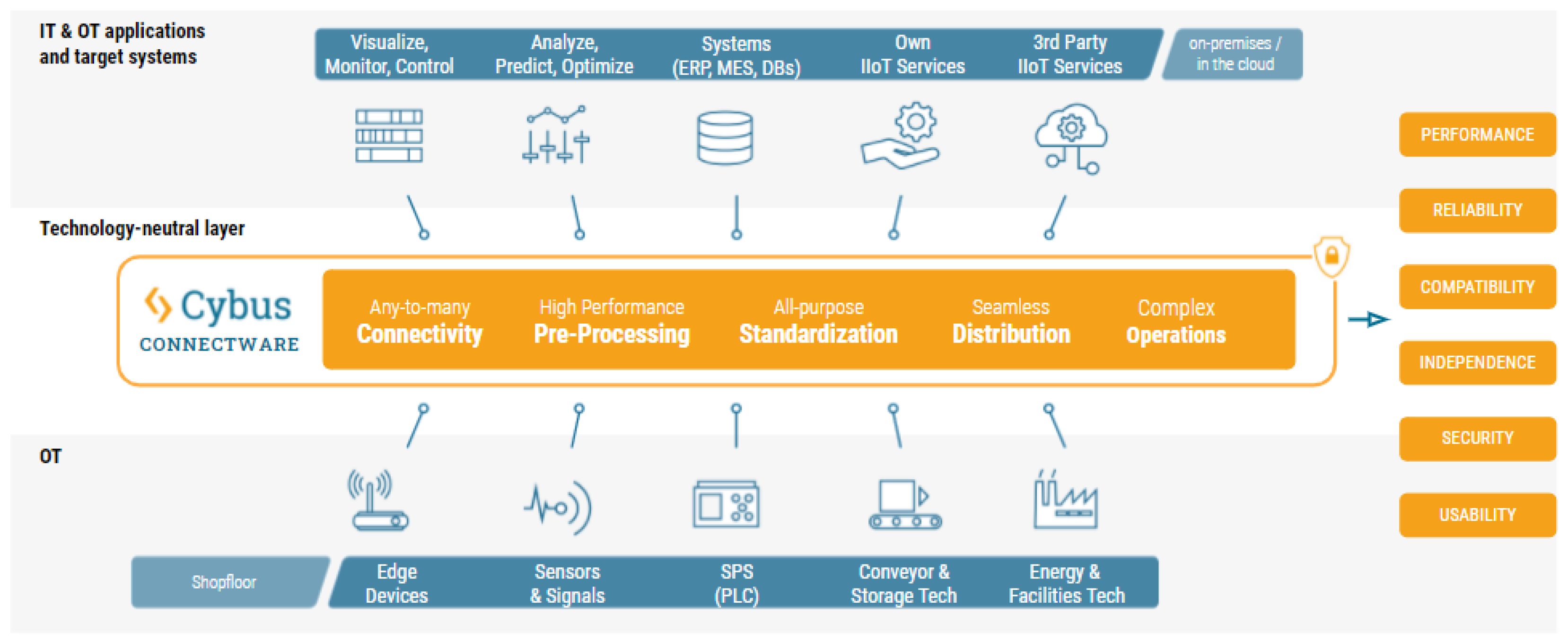
For the brownfield scenario, a five-axis milling center (DMG 100 U duoBLOCK) was used [13]. The machine was equipped with a rotating pallet changer to allow changeover preparations in parallel to the production time (Figure 2, right). In order to implement the combined approach, establishing a connection to access data from the NC HEIDENHAIN Mill Plus IT (Version 530) was essential. Unfortunately, it was not realizable on this machine, as the Mill Plus IT NC is not supported by the HEIDENHAIN DNC interface [39]. Consequently, for both the combined and greenfield scenarios, it became necessary to identify an alternative machine with comparable features. The objective was to ensure comparability with previous research, leading to the search for a milling machine equipped with five-axis kinematics and support for the HEIDENHAIN DNC interface.
Figure 2 (left) shows the HERMLE C600 U milling machine selected for both the combined and greenfield scenarios. The machine also has five-axis kinematics and is equipped with an NC HEIDENHAIN iTNC 530, which is compatible with the HEIDENHAIN DNC interface. Compared to the previously used DMG 100 U duoBLOCK, the HERMLE machine has no rotating pallet changer.
The mentioned machine tools were located on the shopfloor of Pabst Komponentenfertigung GmbH from the OBerA project consortium. These production machines operate on multi-shift schedules to process regular customer orders.

2.3. Connectivity

Section 1.1 described the fact that the connectivity approach for a brownfield environment must enable the simple integration of many different sensors and their heterogeneous interfaces. For the greenfield scenario, devices, such as machine controls, are already equipped with hardware and software to make their machine states available for other applications. In the following sections, the chosen setups for brownfield (Section 2.3.1), greenfield (Section 2.3.2), and the combined approach (Section 2.3.3) are explained.

2.3.1. Brownfield Setup

For the brownfield setup, it was necessary to establish a flexible platform to integrate very different sensor types and interfaces. The aim was to establish a stand-alone solution for the external sensor setup and not to connect sensors to the machine’s NC. For this purpose, a Simatic IoT2040 gateway from Siemens for installation in a switch cabinet was chosen. It offers low-level sensor interfaces, such as RS232 and RS485 ports, as well as GPIO, including I2C and SPI support. An integrated web service allows for the transmission of data, e.g., via the MQTT protocol (integrated Node-RED software (Latest version: v3.1.3 (npm))).
Additionally, an IO-Link master AL1350 from IFM was selected. IO-Link is a standardized interface to connect sensors and actuators. It realizes bidirectional communication between the sensor/actuator and PLC/NC control and enables the identification and transmission of parameters, processes, events, and diagnostic data ([40], p. 27). A large selection of industry-grade sensors is available for IO-Link. The IO-Link-master can be connected to field buses. In the case of the chosen IFM IO-Link master, a web service is also integrated into the device, allowing it to transmit data using the MQTT protocol.
The data are aggregated on an Intel Next Unit of Computing (NUC) mini PC using the software Node-RED. Then, the data are transmitted to an SQL database via a long-term evolution (LTE) router.
Overall, this solution covers a wide range of different sensors and is not dependent on the used machine or its NC.

2.3.2. Greenfield Setup

A generalized software interface for the data acquisition process was used instead of using the proprietary software interfaces from the NC manufacturer HEIDENHAIN. For this research, Cybus Connectware was chosen for the connection of the NC (see also Section 2.2.4). It offers the possibility to acquire data from a broad range of NCs from the OBerA consortium.
Cybus Connectware is a manufacturing data platform that bridges the gap between operation technology (OT) on the shop floor and information technology (IT) by building a universal data architecture. This enables widespread and secure data flow between industrial hardware and IT systems and services [41]. Within this environment, Cybus Connectware acts as a technology-neutral layer between the IT and OT levels in the automation stack (see Figure 3).
This enables connectivity between various devices on the shop floor, such as sensors, signals, edge devices, and PLCs. At a controller level, Cybus Connectware can transmit data bidirectionally via the typical industrial communication protocols, such as OPC UA, Modbus/TCP, Siemens S7, Ethernet/IP, FANUC FOCAS, HEIDENHAIN DNC, and many more [41,43]. Furthermore, Cybus Connectware has the ability to connect to IT applications and systems, such as ERP, a manufacturing execution system (MES), and databases, and custom and third-party industrial Internet of Things (IIoT) services. This setup allows any-to-any communication and data flow for shop floor devices towards enterprise IT systems and vice versa. Using Cybus Connectware as a manufacturing data platform allows for a factory-wide data architecture that receives live data from the shop floor and manages access control as well as the distribution of data to users or applications in the cloud or on-premises. With DevOps capabilities, such as Ansible [44] and Kubernetes [45], Connectware enables the realization of complex use cases and data operations regarding the possibilities of Industry 4.0. Within Cybus Connectware, the hardware parameters are addressed via industry protocol schemes and are mapped into configurable hierarchical names that reflect individual accessible topics on an MQTT-based message broker [41]. Data access is secured on a user-based level by an authentication and authorization system that handles data access per accessed parameter. An entire set of industry protocols, parameter mappings, the corresponding access authentication and authorization schemes, and optional plugin-like applications for local pre- or post-processing can be bundled into so-called Services [41]. Once created, Services can be deployed to the host running Cybus Connectware via configurable text-based Yet Another Markup Language (YAML) files [46], allowing for easy and highly automatable installation. Cybus Connectware is equipped with a browser-based web interface for administering and configuring data endpoints, installing and managing services to implement various use cases, and harvesting the production data [41]. The application of Cybus Connectware is not limited to manufacturing use cases (e.g., [47]). It can also be applied to increase sustainability, e.g., to reduce accidents and waste and increase energy efficiency [48].
For the practical setup of this research work, a Cybus agent software collected the NC data over the HEIDENHAIN DNC interface and transported it to the Azure cloud using the MQTT protocol (see Figure 4). The installation of the Cybus Connectware was located in the Azure cloud. There, the integrated software Node-RED was used to transmit the data to an SQL database for storage. The requirements for the Azure cloud are a 64-bit CPU, 4 GB RAM, and 32 GB hard drive [49].

2.3.3. Combined Setup

The interfaces outlined in Section 2.3.1 and Section 2.3.2 were used concurrently in the combined setup. Regarding the implementation effort, this scenario is presumed to be the most complex. However, this situation may frequently occur in real-world environments, particularly when old machines are replaced and a brownfield application is still operating while being enhanced with the capabilities of a new machine.

3. Methods

In this section, the focus is set on sensor selection methods for the different approaches (Section 3.1). Then, the selection of the ML algorithms to model the use case of a changeover detector is discussed (Section 3.2), and the used performance metrics for the ML models (Section 3.3) are described.

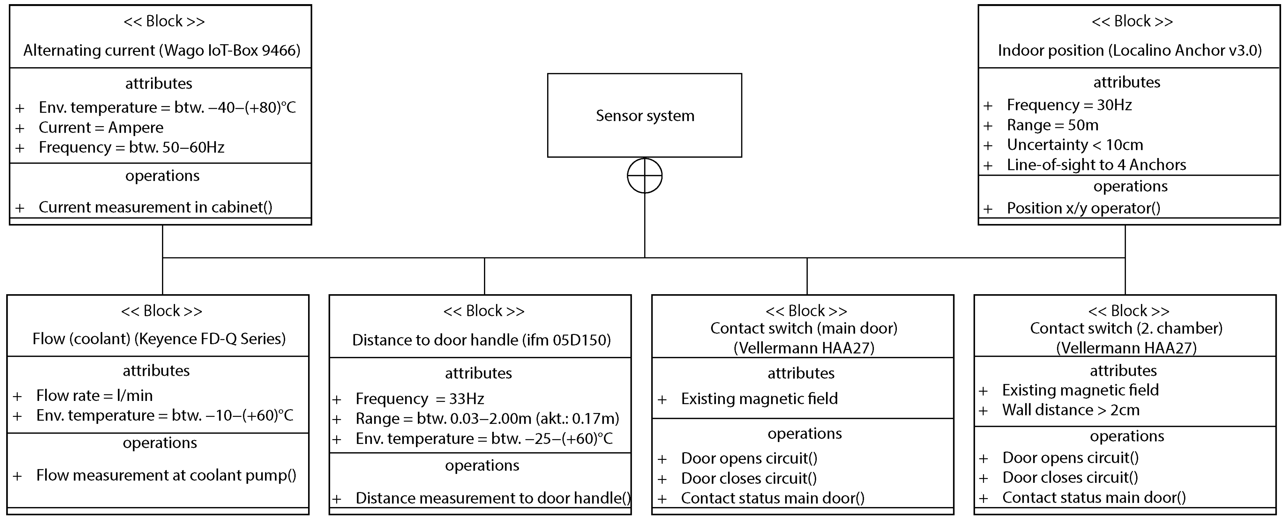
3.1. Sensor Selection Methods

The selection of the right data sources for optimization tasks can be challenging, but this problem is basically understood, e.g., from the Six Sigma approach, where data collection plans are generated [50]. A prerequisite for creating data collection plans is an understanding of the output and input variables for optimization. The output variables are the target of the optimization and are influenced by the input variable. During the optimization process, suited settings for the input variables are determined to generate the optimal output.
In Six Sigma, a general understanding of input and output variables is collected by a detailed description and definition of the process that is about to be optimized (supplier, input, process, output, customer diagram (SIPOC), and process map) [51]. Then, an understanding of the input and output variables can be generated by a cause-and-effect matrix (CE-Matrix) or cause and effect diagrams (Fishbone or Ishikawa diagram) ([52], p. 112ff).
On this basis, prioritization of the inputs can be made. Often, a data acquisition plan is created for this purpose. From the highest-rated inputs, hypotheses about the effectiveness of the inputs can be formulated. These hypotheses must then be accepted or rejected via analyses and interpretation of the results. These hypotheses’ test decisions then determine whether the corresponding inputs are included in the selection ([52], p. 136ff).
From the point of view of the measurement, the input variable, so far, is not equal to a specific sensor. It can be considered a measurand. A measurement is, therefore, a sequence of operations to determine a value for the measurand. A result of a measurement also includes information about the uncertainty of measurement [53]. The measurement uncertainty is a key selection criterion when choosing a specific sensor. There are several metrics available to quantify the uncertainty of a sensor, e.g., measurement system analysis (MSA) [54]. A rule of thumb is “the golden rule of metrology”: the measurement uncertainty of a sensor should be one-tenth of the tolerance to be measured [55].
The methodical approach for selecting a sensor can be summarized with the following steps:
1.
Achieve an understanding of the optimization task (e.g., SIPOC, process map);
2.
Understand the relations between the input and output variables (e.g., CE-Matrix, Ishikawa);
3.
Prioritize the input variables (e.g., CE-Matrix);
4.
Find a set of suited sensors for the measurand from these input variables (e.g., lists with measurement principles and sensor manuals);
5.
Evaluate the sensors (e.g., MSA and uncertainty budget);
6.
Conduct hypothesis tests for the most important inputs (e.g., data acquisition plan and statistical tests).
An ML task usually has a target variable, Y, which depends on several independent variables, x i . The dependent variables correspond to the output variables described above, and the independent variables correspond to the input variables. The independent variables need to be measured to deliver data for the training of the ML model. For supervised ML, the target variable needs to be measured. The selection of possible sensors for the independent variables, x i , should be supported by the expert knowledge of data scientists and domain experts, as described for the classical Six Sigma approach above.
Existing data sources are referred to as passive sources in Six Sigma, while the data sources resulting from experiments or hypothesis tests are referred to as active sources ([52], p. 44). One advantage of passive sources is their availability, as these sources already exist in the operational context. However, these sources have the disadvantage that these variables are pre-selected under a certain context and may also be post-processed and filtered. Active sources require more effort to determine but are geared toward the optimization task and, therefore, offer more accuracy. This distinction between active and passive sources becomes important when discussing the sensor selection approach for the brownfield (Section 3.1.1) and greenfield approaches (Section 3.1.2).
In the following text, the terms “target variable” for Y and “independent variable” for x i are used. For the use case of a changeover detector, the target variable Y is a decision variable, containing the two elements “Changeover”, if a changeover is detected, or “Production” (see Section 2.1). The variable Y is assigned to the measurements of x i in a so-called labeling process. The labels for variable Y were assigned while recording and supervising practical changeover processes on the shop floor. In the following sections, the sensor selection for the variables for x i for each approach is explained.

3.1.1. Brownfield Selection Methods

Section 1.1 describes how the necessary sensors are not yet integrated and need to be selected in a brownfield scenario. Considering the above-described terminology, they can be considered active sources, which require effort for selection but offer a good adaption to the optimization task.
For the use case of a changeover detector (see Section 2.1), the described steps from above can be considered in the sensor selection process: At first, a general understanding needs to be achieved, and sensors to acquire data for the independent variables, x i , need to be chosen (see Section 3.1).
In order to gain insight into the process, an alternative tool to those mentioned in Section 3.1 is utilized: the so-called systems modeling language (SysML). The SysML, which is used in system engineering in particular, provides support for the formal description of structures, behaviors, and requirements ([56], p. 30). Within the SysML framework, multiple diagram types are defined. In order to achieve an understanding of the optimization task (Step 1, see Section 3.1), the requirement diagram, use case diagram, activity diagram, and block definition diagram were used. The exemplary activity (Figure 5) and block definition diagrams are shown in Figure 6. While the activity diagram can serve the purpose of a process map, the block definition diagram can offer an added value for the selection of specific sensors; for each selected sensor, the measurand, as well as information on the measurement operation, were described (Step 4).
In order to understand the input and output variables (Step 2), as well as the prioritization of variables (Step 3), a CE-Matrix was also created (see Table 3). The steps of the changeover process were taken from the activity diagram, and the possible measurands from the block definition diagram were assigned. Then, this was discussed with domain experts to see if the specific changeover step can be detected by the underlying sensor. From these discussions, the set of suited sensors was derived (see Table 4).
The selected external sensors have the disadvantage of being affected by environmental conditions, such as heat, humidity, and vibrations. When externally mounted and visible, they can also be regarded as surveillance devices by the workforce. This is especially important for the tracking of the operator position. Here, it must be assured that sensor recordings are anonymized and comply with data security standards.
For the evaluation step of the sensors (Step 5), standardized testing methods exist. Moreover, sensors with binary testing decisions, such as “on/off”, can be checked. For the sake of readability, these methods are not described in detail here. For the indoor positioning system (PS), a measurement uncertainty analysis was carried out [57]. As the hypothesis tests (Step 6) were correlation tests, principal component analysis (PCA) and t-distributed stochastic neighbor embedding (t-SNE) analysis were conducted [13].

3.1.2. Greenfield Selection Methods

The HERMLE C600 U milling machine with its HEIDENHAIN iTNC 530 NC offers more than 400 potential features over the Cybus Connectware for ML models as input or dependent variables xi. Revisiting the concept of active and passive sources, the Cybus Connectware can be regarded as a passive source. The choice of 400 potential features can be regarded as pre-selection (see Section 3.1) in the context of the milling machine, as the interface exports all available machine variables. Data for these variables can originate from NC-provided sensors, which are physically connected to the NC. Additionally, NC-provided variables, such as the current DNC mode, are exported.
With the switch from the DMG milling machine to the HERMLE machine for the greenfield approach, it was necessary to revisit the process steps of the changeover phases and slightly adapt the documents from Step 1 (understanding the optimization task) and Step 2 (relations between the inputs and output) of brownfield selection; the new machine cannot swivel the palette changer; therefore, the step description was changed to ”putting/retrieving tools directly into/from the spindle”. Additionally, two final steps were added for general quality control and work-piece quality control. For Step 3, a team of domain experts then selected 19 from the available 400 features, sorting out any duplicates and focusing on the process variables that could be related to the use case of machine changeover (see Table 5).
This list of nineteen pre-selected features was reduced to eight (Step 4); at first, a basic statistical analysis was carried out to evaluate the minimum/maximum values and the standard deviation of the feature. CabinDoorLockSide, SpindleApproval, and OverrideSpindle showed no changes in their values over the observation period and were excluded. Then, a correlation analysis and a calculation of the importance of individual features (permutation feature importance (PFI)) were conducted (Step 6). The remaining features were DoorStatus Tooling, DriveStatus, FeedRate, OverrideFeed, PocketTable, ProgramStatus, SpindleSpeed, and ToolNumber. Most of these features are related to the milling process of the HERMLE machine. For the selection of sensors in the greenfield scenario, it can be summarized that by using only the interface of the NC, a pre-selection concerning the context of the milling machine was made. This pre-selection was further adjusted by domain experts, and a fine selection was made using feature selection approaches.
For the evaluation of the sensors (Step 5), the following was found:
1.
DoorStatus is a binary testing decision and can be checked with standardized methods;
2.
DriveStatus, PocketTable, ProgramStatus, and OverrideFeed represent status information from the NC and are difficult to check;
3.
FeedRate and SpindleSpeed are NC parameters for the milling process and can be checked with additional testing efforts (external testing equipment is necessary).
Though it is possible, from a theoretical point of view, to verify the status information and the milling process parameters from the NC, this is often not conducted by the practitioners. Using data from these sensors poses a risk to the quality of the ML model because the uncertainty of the measurement remains unknown and can impact the quality metrics of the ML model (see Section 3.3 and Section 4). In order to evaluate these consequences for the practitioners later on (see Section 5), no further investigations were carried out here. At this point, it can be summarized that model inaccuracies that can arise due to the pre-selection problem of passive sources can be aggravated by a missing evaluation of sensor suitability.

3.1.3. Combined Approach Selection Methods

The combined approach consists, initially, of the selected sensors from the brownfield (see Section 2.3.1) and greenfield (see Section 2.3.2) approaches. The external sensors for coolant flow and the door contacts were left out because they were available from the NC (see Table 6, NC-provided, replacing, initial selection). The indoor PS and the sensor for the power consumption remained in the selection for the NC-external sensors. Newly added NC-provided sensors to the initial selection were the same sensors as those described for the greenfield approach (see Table 5, initial selection). After refining the sensor selection, as described above, the final selection of the sensors for the combined approach consists of the indoor PS and the sensors from the final selection of the greenfield approach (see Table 5, final selection). The feature PowerConsumption was left out as it was directly correlated to SpindleSpeed and DriveStatus.

3.2. Chosen Machine Learning Algorithms

In [13], it was confirmed by the authors that random forest algorithms are well suited for the described machine learning (ML) classification task. For further research work, extra trees were also selected for the training of the ML models. Extremely randomized trees (ERTs) or extra trees are similar to random forests but have advantages, i.e., faster computation time and reduced variance [58]. In [59], it was stated that when random forest algorithms perform well, gradient boosting can also be taken into consideration. These algorithms show advantages in terms of training speed and generalization. Therefore, CatBoost, LightGBM, and XGBoost were also selected for the training.
For the ML algorithms random forest, CatBoost, and XGBoost, hyperparameter optimization was conducted. For LightGBM and extra trees, hyperparameter optimization showed no improvements, and therefore, standard parameters were used. For details, please consult the provided source code (see Data Availability Statement) and Appendix A.

3.3. Performance Metrics

Several metrics exist for the evaluation of ML models. A popular metric is the F1 score. The value of the F1 score ranges between 0 and 1. For a classification task, a value of 0 indicates that none of the data points were correctly assigned to the right class. A value of 1 indicates that all data points were classified correctly ([60], p. 430).
For imbalanced datasets, the F1 score is regarded as problematic. In this case, the Matthews correlation coefficient (MCC) is preferred instead ([61], p. 10, and [62]). Like the F1 score, the MCC ranges from 0 to 1.
Data points are considered imbalanced when the quantity of data points is differently distributed in the groups that are to be classified. Figure 7 shows the occurrences of the two phases, “Production” and “Changeover”. It can be seen that the “Production” phase is slightly more frequent in the data than the “Changeover” phase. Therefore, in this paper, the F1 score and the MCC were used together to compare the quality of the ML models. For improved readability, the ranges of the F1 score and the MCC were converted into percentage values (0 as 0% and 1 as 100%).

4. Results

This section evaluates the results from the implemented scenarios from the use case. First, the qualitative findings from the implementation are summarized in Section 4.1. Then, the performance metric results for the ML models are presented in Section 4.2.

4.1. General Findings from Implementation

In Section 1.2, an implementation process for ML models proposed by [4] was introduced. Regarding this implementation workflow, there were noticeable differences between the greenfield and brownfield approaches (see Figure 8). For the brownfield approach, usually, the workflow starts with the definition of the optimization goal and the derivation of a corresponding target or output variable. Afterward, the independent or input variables, which are expressed in combination with the output variable, are elaborated. Then, a relationship between the input and output variables can be determined (here, by ML models) (see also Section 3.1).
There already exists a selection of input variables for the greenfield approach, which are available through up-to-date machine interfaces. This selection needs to be refined during feature selection. Using a selection of machine interface variables also incorporates an implicit assumption that this selection can somehow express the output variable of the optimization.
In the following subsections, the methodical approach for selecting sensors/features from Section 3.1 is discussed individually for all three scenarios.

4.1.1. Brownfield Findings

For the brownfield scenario, the understanding of the optimization task was generated through the generation of SysML diagrams (Step 1). Here, the block definition diagram has already helped find a set of suitable sensors for the input variables (Step 4). The relationship between the input and output variables, as well as the prioritization of variables, was achieved by the application of a CE-Matrix (Step 2 + 3). For the evaluation of sensors (Step 5), standardized testing methods were applied, and hypothesis tests were conducted (Step 6).
Overall, it was possible to follow the planned methodological procedure in full. With regard to the sequence of steps, the use of SysML as a support tool meant that Step 4 could be conducted earlier.

4.1.2. Greenfield Findings

For the greenfield scenario, a process for understanding the optimization task (Step 1) and the relations between the input and output variables (Step 2) was conducted. As Cybus Connectware offered more than 400 potential features, the prioritization of the input variables (Step 3) was important for the greenfield scenario. This prioritization started with the pre-selection of 19 features by domain experts (Step 3). The further reduction in the features to a final set of eight was carried out using feature selection techniques (Step 4).
In the greenfield scenario, the machine interfaces provide data regardless of if the underlying sensor is suited in terms of measurement uncertainty, which is checked only during Step 5. The features that are related to unsuited sensors need to be omitted. The situation of omitting features may cause conflicts with Step 4; during this step, the technique of permutation feature importance (PFI) was used to reduce the number of features. This technique generates preliminary models with specific combinations of features and derives feature importance. If a sensor in Step 5 is omitted, in this case, Step 4 needs to also be revisited without this feature. Depending on the importance of the feature, the entire remaining set of features might change. While conducting Step 5, it also turned out that the features that belong to the internal sensors of the machine are difficult to check. The practitioner might be tempted, in this case, to skip this step. During Step 6, correlation tests, PCA and t-SNE, were conducted to analyze whether the entire feature set is suitable for modeling.
To summarize, the high quantity of available features in the greenfield scenario underlines the importance of Steps 3 and 4 to reduce their number. Regarding Step 5, problems can arise as a pre-selection of features already exists, which, thus, defines the underlying sensor selection. However, the sensor suitability check only takes place after the pre-selection and may be skipped by the practitioner due to convenience.

4.1.3. Combined Approach Findings

The feature set of the combined scenario consisted of the x/y position from the indoor PS and features from the Cybus Connectware interface. The external sensors from the brownfield scenario were regarded as being the same as the features from the Connectware interface. Therefore, no more specific findings from the implementation process were noticed.

4.2. Performance Metrics Results

In this subsection, we present the metrics for the different ML algorithms, which were trained with the recorded data for the brownfield (Section 4.2.1), combined (Section 4.2.2), and greenfield (Section 4.2.3) approaches. Each algorithm is evaluated by using the F1 score and MCC metric.

4.2.1. Brownfield Results

In Figure 9, the results for the brownfield approach are shown. The highest F1 scores were achieved for the extra trees (97.4%) and the random forest algorithms (97.25). The CatBoost algorithm shows the lowest F1 score, with 95.37%. In comparison to the F1 score, the MCC value always shows lower percentages. The difference between F1 score and MCC ranges from 2.57% (extra trees) to 4.57% for the CatBoost algorithms. Overall, the performance metrics of all algorithms are moderate, showing F1 scores over 95.37% but an MCC of only 90.8%.

4.2.2. Combined Approach Results

Figure 10 shows the results of the combined approaches. The highest F1 scores were achieved by the extra trees, random forest, and XGBoost algorithms (99.63). The lowest F1 scores were achieved by the CatBoost (99.57%) and the LightGBM (99.52%) algorithms. In comparison to the F1 score, the MCC value also shows lower percentages. However, compared to the brownfield approach, the gap between the F1 score and MCC is much smaller and ranges from 0.57% (extra trees, random forest, and XGBoost) to 0.44% for CatBoost and 0.48% for LightGBM. Overall, the performance metrics of all algorithms are excellent, showing F1 scores over 99.52% and over 99.04% for the MCC.

4.2.3. Greenfield Results

In Figure 11, the results for the greenfield approach are shown. The highest F1 score was achieved by the XGBoost algorithm (98.83%). The lowest F1 scores were obtained by the extra trees (98.58%) and the random forest (98.65%) algorithms. In comparison to the F1 score, the MCC value also shows lower percentages, but like the combined approach, the gap between the F1 score and MCC is much smaller than in the brownfield approach and ranges from 1.2% for LightGBM to 1.41% for extra trees. Overall, the performance metrics of all algorithms are very good, showing F1 scores over 98.58% and over 97.17% for the MCC.

5. Discussion

In Figure 12, the F1 scores from the previous chapters are summarized. For the brownfield approach, the F1 scores range from a minimum of 95.37% to a maximum of 97.4%. From all scenarios, the brownfield scenario has the lowest F1 scores with an absolute range of 2.03%.
When the sensor/feature selection from the combined approach is applied to training the ML models, the F1 scores become almost optimal, with values from 99.52% to 99.63% and a very small range of 0.11%. The difference between the sensor/feature set of the brownfield approach is that the process parameters, such as the feed rate of the milling process, were also taken into account. Additional machine parameters, like the status of door switches, were directly recorded through NC variables. The external Rogowsky sensors for power consumption were substituted by correlating NC variables. For the classification task between changeover and production, better results were generated by also considering the process parameters of the milling process. As an external sensor, just the indoor PS, measuring the x/y position of the operator, remained as part of the ML model.
The F1 scores for the greenfield approach are slightly lower when compared to the combined approach: the F1 scores have a minimum of 98.58% and a maximum of 98.83%. The range of 0.25% between these values is twice as high as that of the combined approach but around a factor of 10 better than that of the brownfield approach. When comparing the best model from the combined approach (extra trees, random forest, and XGBoost: 99.62%) to the best model from the greenfield approach (XGBoost: 98.83%), the external indoor PS sensor in the combined approach seems to be responsible for a performance difference of 0.79%.
As this underlying data set is slightly imbalanced, different methods could be considered to improve the classification results, for example, over- or undersampling the classes to minimize the imbalance [63]. Additionally, a genetic algorithm could be utilized to create more data points [64]. These methods were not used, as the dataset is not strongly imbalanced.
All approaches need experts to select the sensors/features. For the combined and greenfield approach, this selection could be automated. For example, using all available variables and conducting a PFI to identify the most important features. The PFI can be combined with all ML algorithms, such as neural networks or random forests. Another approach would be to use AutoML to select features [65]. These methods can only be used when there are recorded data. For the brownfield approach, this is only applicable if there are many external sensors installed.

6. Conclusions and Further Research

In this section, the conclusions are derived (Section 6.1), and an outlook for further research is given (Section 6.1).

6.1. Conclusions

The brownfield approach differs from the combined approach primarily in that none of the parameters of the milling process that are available in the NC were included in the classification task. In Step 13 of the description of the changeover process (see Table 3), the NC program and the parameters of the milling process are optimized. Because only external sensors were explicitly used in the brownfield approach, the activities concerning the NC can only be recorded indirectly, e.g., via the operator position in front of the NC. Overall, the ML models of the brownfield approach show the worst performance compared to the other approaches. Nevertheless, random forest and extra trees can achieve good results above 97%. This also confirms that extra trees are suitable when random forest algorithms show good results. However, the range in the performances of all the ML algorithms indicates that the selected input variables and, thus, external sensors do not yet cover the changeover process sufficiently well. This is also implied by the biggest differences between the F1 scores and MCC values of all approaches.
If the combined approach is compared with the greenfield approach, the position detection of the employee by the external indoor PS is omitted. The loss of this information slightly degrades the excellent results of the combined approach. Although the influence of the employee’s position on the setup is, therefore, evident, it can be partially compensated by the information from the milling-related parameters. For the modeling of a setup detector, however, the use of process parameters from an NC seems, overall, to be advisable.
For production and technology-related optimization tasks, such as the setup detector, a brownfield approach based only on external sensors appears to be too inaccurate overall. However, in this case, the application of the changeover detector decides whether a 97% F1 score is sufficient. The greenfield approach, based solely on input variables from the controller, delivers better results here. However, the choice of possible variables is much larger here, and the quality of sensor readings can often not be verified or can be only with great effort. In addition to the lack of position information from the operator, these two reasons may have contributed to the greenfield approach performing slightly worse than the combined approach. The good results for the combined approach imply that it might be beneficial to incorporate features that are only indirectly related to the optimization task, like the position of the operator. For other machining operations, e.g., injection plastic molding, the movement of the molds might be considered as a feature.
The presented methodical approach for selecting sensors shows applicability for all approaches (first research question). The end users of this approach are either manufacturing engineers who typically conduct data-driven improvement projects (Six Sigma) or data scientists who conduct digitization projects. The heterogeneity of the interfaces in the brownfield approach poses challenges for both groups, as customization efforts have to be made. In the greenfield approach, software suites, such as Cybus Connectware, make it easier to roll out ML applications based on shopfloor data. Automatized feature selection methods can be used efficiently here. The approach described can ensure, in this case, that the selection of suitable data sources is reliable. In the greenfield approach, the suitability of the internal sensors should be ensured as far as possible as part of regular measurement device monitoring in order to be able to provide reliable data via interfaces.
Though the results for the brownfield approach were worse than for the greenfield and combined approaches, the described methodical approach can help to avoid ML models with low quality, e.g., below 90% MCC (second research question).
In the case of the brownfield approach, the domain experts made the assumption that the selected sensor set was suited for the ML task. This assumption became questionable after additional features from the NC were entered into the combined and greenfield approaches and showed better results. Despite the efforts for the creation of the ML models, the model creation and validation itself can be interpreted as a hypothesis test in terms of the methodical approach for selecting sensors (Step 6). For the greenfield approach, it can be concluded that domain experts might also assume that the rich availability of features from an NC guarantees the best performance results for ML models. Moreover, for this approach, the model creation and validation can serve as a hypothesis test. However, the changeover use case also shows that 400 features should be pre-selected instead of spending computing resources on ML models with large feature sets. Overall, it can be pointed out that the decisions of the domain experts have an impact on the results. In the case of the brownfield approach, the selection process for sensors is strongly dependent on their creativity, problem-solving, and methodical competence. For the greenfield approach, feature selection algorithms might reduce their impact, as feature selection algorithms can support the sorting out of variables. The challenge here is for the domain experts to check whether the feature set contains enough information for the modeling despite a rich choice of features.

6.2. Further Research

It was shown that the integration of specific information, such as milling parameters, is particularly important if changeover detectors are to be created for other machining processes. In future research work, the modeling of other machining processes, such as turning, is to be pursued further. The investigation should also focus on a precise evaluation of the contribution of the specific process parameters in order to improve the transferability of the approach from milling to other machining processes.
In an operational context, employee tracking is problematic. Operators may feel controlled and adjust their operational activities accordingly. The results for the greenfield approach show that the indoor PS can be omitted, but this causes a slight decrease in the quality metrics of the ML models. However, further work is needed to check whether the accuracy of the greenfield models is still sufficient for specific applications, i.e., time data updates in ERP systems.

Author Contributions

B.E.: conceptualization, methodology, validation, formal analysis, investigation, resources, writing—original draft, writing—review and editing, visualization, supervision, project administration, and funding acquisition. A.-M.S.: conceptualization, methodology, software, validation, formal analysis, data curation, writing—original draft, writing—review and editing, and visualization. L.T.: writing—original draft and writing—review and editing. J.S.: formal analysis and writing—review and editing. All authors have read and agreed to the published version of the manuscript.

Funding

This research was funded by the state of Bavaria (Bayerisches Staatsministerium für Wirtschaft, Landesentwicklung und Energie, grant number IUK 530/10).

Data Availability Statement

The research data and source code is available on Git Hub: https://github.com/SuperAms/machine_learning_models_in_manufacturing.

Acknowledgments

The authors gratefully thank Pabst Komponentenfertigung GmbH and Cybus GmbH for their contribution to the research.

Conflicts of Interest

Author Lukas Theilacker was employed by the company Cybus GmbH. The remaining authors declare that the research was conducted in the absence of any commercial or financial relationships that could be construed as a potential conflict of interest.

Abbreviations

The following abbreviations are used in this manuscript:
CE-Matrixcause-and-effect matrix
DNCdistributed numerical control
ERPenterprise resource planning
PSpositioning system
IIoTindustrial Internet of Things
ITinformation technology
LTElong-term evolution
MCCMatthews correlation coefficient
MESmanufacturing execution system
MLmachine learning
MQTTmessage queuing telemetry transport
MSAmeasurement system analysis
NCnumerical control
NUCNext Unit of Computing
OBerAOptimization of Processes and Machine Tools through Provision, Analysis and
Target/Actual Comparison of Production Data
OToperation technology
PCAprincipal component analysis
PFIpermutation feature importance
PLCprogrammable logic controller
OPC UAOpen Platform Communications Unified Architecture
SIPOCsupplier, input, process, output, customer diagram
SMEsmall and medium-sized enterprise
SQLstructured query language
SysMLsystems modeling language
t-SNEt-distributed stochastic neighbor embedding
umatiuniversal machine technology interface
VMvirtual machine
YAMLYet Another Markup Language

Appendix A. Hyperparameters of Algorithms

For the brownfield approach, the hyperparameters were tuned in previous research using a grid search; therefore, the parameters for the random forest algorithm were used [13]. They are the following:
  • Number of estimators (trees): 30;
  • Bootstrap: False;
  • Max. depth of tree: 30;
  • Min. samples at leaf: 1;
  • Min. samples to split: 2.
For the other algorithms, the tuned hyperparameters of the combined approach were used, as they provided better results. A separate grid search was not conducted. The standard parameters of the Python scikit-learn and lightgbm packages were used for the extra trees and LightGBM algorithms for all three approaches. For the combined and greenfield approach, the standard parameters for random forest were also used. Table A1 shows the hyperparameters for the CatBoost and XGBoost algorithms.
Table A1. CatBoost and XGBoost hyperparameters for the combined and greenfield approaches.
CatBoostXGBoost
iterations: 260objective: binary:logistic
depth: 9colsample_bytree: 0.7
loss_function: Loglosslearning_rate: 0.4
random_strength: 0.7max_depth: 9
eta: 0.3n_estimators: 170
sampling_frequency: PerTreereg_alpha: 0.005
scale_pos_weight: 3.3
subsample: 0.9

References

  1. Europäische Kommission—Empfehlung der Kommission vom 6. Mai 2003 Betreffend die Definition der Kleinstunternehmen Sowie der Kleinen und Mittleren Unternehmen. 2003. Available online: https://eur-lex.europa.eu/legal-content/DE/TXT/PDF/?uri=CELEX:32003H0361&fro=DE (accessed on 29 July 2021).
  2. Säfsten, K.; Harlin, U.; Johansen, K.; Larsson, L.; Vult von Steyern, C.; Öhrwall Rönnbäck, A. Towards Resilient and Sustainable Production Systems: A Research Agenda. In SPS2022; IOS Press: Amsterdam, The Netherlands, 2022; pp. 768–780. [Google Scholar]
  3. Thornton, G.; Franz, M.; Edwards, D.; Pahlen, G.; Nathanail, P. The challenge of sustainability: Incentives for brownfield regeneration in Europe. Environ. Sci. Policy 2007, 10, 116–134. [Google Scholar] [CrossRef]
  4. Tran, T.A.; Ruppert, T.; Eigner, G.; Abonyi, J. Retrofitting-based development of brownfield industry 4.0 and industry 5.0 solutions. IEEE Access 2022, 10, 64348–64374. [Google Scholar] [CrossRef]
  5. Etz, D.; Brantner, H.; Kastner, W. Smart manufacturing retrofit for Brownfield systems. Procedia Manuf. 2020, 42, 327–332. [Google Scholar] [CrossRef]
  6. Strauß, P.; Schmitz, M.; Wöstmann, R.; Deuse, J. Enabling of predictive maintenance in the brownfield through low-cost sensors, an IIoT-architecture and machine learning. In Proceedings of the 2018 IEEE International Conference on Big Data (Big Data), Seattle, WA, USA, 10–13 December 2018; pp. 1474–1483. [Google Scholar]
  7. O’Donovan, P.; Gallagher, C.; Leahy, K.; O’Sullivan, D.T. A comparison of fog and cloud computing cyber-physical interfaces for Industry 4.0 real-time embedded machine learning engineering applications. Comput. Ind. 2019, 110, 12–35. [Google Scholar] [CrossRef]
  8. Miao, J.; Niu, L. A Survey on Feature Selection. Procedia Comput. Sci. 2016, 91, 919–926. [Google Scholar] [CrossRef]
  9. Amershi, S.; Begel, A.; Bird, C.; DeLine, R.; Gall, H.; Kamar, E.; Nagappan, N.; Nushi, B.; Zimmermann, T. Software Engineering for Machine Learning: A Case Study. In Proceedings of the 2019 IEEE/ACM 41st International Conference on Software Engineering: Software Engineering in Practice (ICSE-SEIP), Montreal, QC, Canada, 25–31 May 2019; pp. 291–300. [Google Scholar] [CrossRef]
  10. Axehill, J.W.; Herzog, E.; Tingström, J.; Bengtsson, M. From Brownfield to Greenfield Development – Understanding and Managing the Transition. INCOSE Int. Symp. 2021, 31, 832–847. [Google Scholar] [CrossRef]
  11. Klaeger, T.; Gottschall, S.; Oehm, L. Data Science on Industrial Data—Today’s Challenges in Brown Field Applications. Challenges 2021, 12, 2. [Google Scholar] [CrossRef]
  12. Runeson, P.; Host, M.; Rainer, A.; Regnell, B. Case Study Research in Software Engineering: Guidelines and Examples; Wiley: Hoboken, NJ, USA, 2012. [Google Scholar]
  13. Miller, E.; Borysenko, V.; Heusinger, M.; Niedner, N.; Engelmann, B.; Schmitt, J. Enhanced Changeover Detection in Industry 4.0 Environments with Machine Learning. Sensors 2021, 21, 5896. [Google Scholar] [CrossRef]
  14. Hu, Z.; Gong, W.; Pedrycz, W.; Li, Y. Deep reinforcement learning assisted co-evolutionary differential evolution for constrained optimization. Swarm Evol. Comput. 2023, 83, 101387. [Google Scholar] [CrossRef]
  15. Zhao, F.; Zhang, H.; Wang, L. A pareto-based discrete jaya algorithm for multiobjective carbon-efficient distributed blocking flow shop scheduling problem. IEEE Trans. Ind. Inform. 2022, 19, 8588–8599. [Google Scholar] [CrossRef]
  16. Han, Y.; Peng, H.; Mei, C.; Cao, L.; Deng, C.; Wang, H.; Wu, Z. Multi-strategy multi-objective differential evolutionary algorithm with reinforcement learning. Knowl.-Based Syst. 2023, 277, 110801. [Google Scholar] [CrossRef]
  17. Engelmann, B.; Schmitt, S.; Miller, E.; Bräutigam, V.; Schmitt, J. Advances in Machine Learning Detecting Changeover Processes in Cyber Physical Production Systems. J. Manuf. Mater. Process. 2020, 4, 108. [Google Scholar] [CrossRef]
  18. Géron, A. Hands-on Machine Learning with Scikit-Learn, Keras, and TensorFlow: Concepts, Tools, and Techniques to Build Intelligent Systems; O’Reilly Media, Inc.: Sebastopol, CA, USA, 2019. [Google Scholar]
  19. Sauer, C.; Eichelberger, H.; Ahmadian, A.S.; Dewes, A.; Jürjens, J. Current Industry 4.0 Platforms—An Overview. IIP-Ecosphere Whitepaper, Leibniz Universität Hannover, Forschungszentrum L3S, Appelstraße 9a, 30167 Hannover, Germany, 2021. Available online: https://zenodo.org/records/4485756 (accessed on 14 January 2024).
  20. Martins, A.; Lucas, J.; Costelha, H.; Neves, C. CNC Machines Integration in Smart Factories using OPC UA. J. Ind. Inf. Integr. 2023, 34, 100482. [Google Scholar] [CrossRef]
  21. Balduzzi, M.; Sortino, F.; Castello, F.; Pierguidi, L. An Empirical Evaluation of CNC Machines in Industry 4.0 (Short Paper). In Proceedings of the International Conference on Critical Information Infrastructures Security, Munich, Germany, 14–16 September 2022; Springer: Cham, Switzerland, 2022; pp. 56–62. [Google Scholar]
  22. Martins, A.; Lucas, J.; Costelha, H.; Neves, C. Developing an OPC UA server for CNC machines. Procedia Comput. Sci. 2021, 180, 561–570. [Google Scholar] [CrossRef]
  23. Ižol, P.; Grešová, Z.; Vrabel’, M.; Brindza, J.; Demko, M. The influence of tool path strategies for 3-and 5-axis milling on the accuracy and roughness of shaped surfaces. Mach. Technol. Mater. 2022, 16, 234–237. [Google Scholar]
  24. Wang, W.T.; Chang, C.H.; Sheng, R.N. The Study on the Implementation of Multi-Axis Cutting & Cyber-Physical System on Unity 3D Platform. In Proceedings of the 2019 IEEE 6th International Conference on Industrial Engineering and Applications (ICIEA), Tokyo, Japan, 12–15 April 2019; pp. 77–80. [Google Scholar]
  25. Trabesinger, S.; Butzerin, A.; Schall, D.; Pichler, R. Analysis of high frequency data of a machine tool via edge computing. Procedia Manuf. 2020, 45, 343–348. [Google Scholar] [CrossRef]
  26. Beşirova, C.; Akhtar, W.; Shahzad, A.; Üresin, U.; Çelikel, S.; İrican, M. Analysis of Machining Process with Data Collection Using Industrial Edge Computing. In Proceedings of the 11th International Congress on Machining, Istanbul, Turkey, 9–11 December 2021. [Google Scholar]
  27. Lutz, B.; Howell, P.; Regulin, D.; Engelmann, B.; Franke, J. Towards Material-Batch-Aware Tool Condition Monitoring. J. Manuf. Mater. Process. 2021, 5, 103. [Google Scholar] [CrossRef]
  28. Lima, F.; Massote, A.A.; Maia, R.F. IoT energy retrofit and the connection of legacy machines inside the industry 4.0 concept. In Proceedings of the IECON 2019—45th Annual Conference of the IEEE Industrial Electronics Society, Lisbon, Portugal, 14–17 October 2019; Volume 1, pp. 5499–5504. [Google Scholar]
  29. Schmid, J.; Vallant, D.; Butzerin, A.; Brillinger, M.; Suschnigg, J.; Pichler, R.; Haas, F. Acquisition of machine tool data via the open source implementation open62541 for OPC-UA. Procedia CIRP 2021, 102, 303–307. [Google Scholar] [CrossRef]
  30. Martínez Ruedas, C.; Adame-Rodríguez, F.J.; Díaz-Cabrera, J.M. A Low-Cost’plug and Play’connectivity and Integration System for SINUMERIK CNC Machines to Join INDUSTRY 4.0. Available online: https://papers.ssrn.com/sol3/papers.cfm?abstract_id=4334474 (accessed on 14 January 2024).
  31. Siemens. Connecting Brownfield Facilities with Siemens MindSphere: Making any Factory a Smart Factory—Learn How to Get It Done. 2022. Available online: https://www.plm.automation.siemens.com/media/global/en/Brownfield%20Connectivity%20with%20MindSphere_tcm27-100928.pdf (accessed on 22 February 2022).
  32. Siemens. MindSphere Architecture. 2021. Available online: https://developer.mindsphere.io/concepts/concept-architecture.html (accessed on 6 December 2021).
  33. FANUC. MT-LINKi: The Easy Way to Monitor Your Production. 2021. Available online: https://www.fanuc.eu/~/media/files/pdf/products/cnc/flyers/mfl-02993-fa-mt-linki/mt-linki-flyer-en.pdf?la=de (accessed on 6 December 2021).
  34. FANUC. FANUC FOCAS Library for Easy Customisation of CNC’s. Available online: https://www.fanuc.eu/de/de/cnc/development-software/focas-development-libraries (accessed on 14 January 2022).
  35. FANUC. FANUC OPC Server. Available online: https://www.fanuc.eu/de/de/cnc/connectivity/opc-server (accessed on 14 January 2022).
  36. DR. JOHANNES HEIDENHAIN GmbH. Connected Machining. 2022. Available online: https://www.heidenhain.de/produkte/digitale-werkstatt/connected-machining (accessed on 13 January 2022).
  37. DR. JOHANNES HEIDENHAIN GmbH. Softwarelösungen. 2022. Available online: https://www.heidenhain.de/produkte/digitale-werkstatt/softwareloesungen (accessed on 13 January 2022).
  38. DR. JOHANNES HEIDENHAIN GmbH. Digitale Werkstatt. 2020. Available online: https://www.heidenhain.de/fileadmin/pdf/de/01_Produkte/Broschueren/BR_Digitale_Werkstatt_ID1329161_de_01.pdf (accessed on 14 January 2022).
  39. DR. JOHANNES HEIDENHAIN GmbH. Connected Machining—Individuelle Lösungen für das Digitale Auftragsmanagement in der Fertigung; Dr.-Johannes-Heidenhain-Straße: Traunreut, Germany, 2017. [Google Scholar]
  40. Uffelmann, J.; Wienzek, P.; Jahn, M. IO-Link—Band 1: Anwendung: Schlüsseltechnologie für Industrie 4.0; Number Bd. 1; Vulkan Verlag: Essen, Germany, 2020. [Google Scholar]
  41. Cybus. Overview. Available online: https://docs.cybus.io/latest/user/overview.html (accessed on 28 January 2022).
  42. Cybus. Cybus Journey. 2022. Available online: https://www.cybus.io/cybus-journey-de/ (accessed on 28 January 2022).
  43. Cybus. Connectivity Portfolio. 2022. Available online: https://www.cybus.io/connectivity-portfolio/ (accessed on 28 January 2022).
  44. Erichsen, J. Connectware Orchestration Using Ansible. 2022. Available online: https://www.cybus.io/learn/connectware-orchestration-using-ansible/ (accessed on 28 January 2022).
  45. Pittig, K. Installing Cybus Connectware on Kubernetes Clusters. 2022. Available online: https://www.cybus.io/learn/installing-cybus-connectware-on-kubernetes-clusters/ (accessed on 28 January 2022).
  46. Evans, J.; Schmeding, D. Service Basics. 2020. Available online: https://www.cybus.io/learn/service-basics/ (accessed on 28 January 2022).
  47. Gudenkauf, S.; Franke, J.; Behrens, J. Features of Event-Driven Message Queuing Architectures in Manufacturing: A Reference Model for Comparison; Gesellschaft für Informatik e.V.: Bonn, Germany, 2023. [Google Scholar]
  48. Reis, J.S.d.M.; Espuny, M.; Nunhes, T.V.; Sampaio, N.A.d.S.; Isaksson, R.; Campos, F.C.d.; Oliveira, O.J.d. Striding towards sustainability: A framework to overcome challenges and explore opportunities through industry 4.0. Sustainability 2021, 13, 5232. [Google Scholar] [CrossRef]
  49. Cybus. System Requirements. 2021. Available online: https://docs.cybus.io/latest/user/requirements.html (accessed on 29 December 2023).
  50. Kwak, Y.H.; Anbari, F.T. Benefits, obstacles, and future of six sigma approach. Technovation 2006, 26, 708–715. [Google Scholar] [CrossRef]
  51. Hassan, R.; Marimuthu, M.; Mahinderjit-Singh, M. Application of Six-Sigma for Process Improvement in Manufacturing Industries: A Case Study. Int. Bus. Manag. 2016, 10, 676–691. [Google Scholar]
  52. Melzer, A. Six Sigma—Kompakt und Praxisnah: Prozessverbesserung Effizient und Erfolgreich Implementieren; Springer Fachmedien Wiesbaden: Wiesbaden, Germany, 2015. [Google Scholar]
  53. Joint Committee for Guides in Metrology. Evaluation of Measurement Data—Guide to the Expression of Uncertainty in Measurement. 2008. Available online: https://www.bipm.org/documents/20126/2071204/JCGM_100_2008_E.pdf/cb0ef43f-baa5-11cf-3f85-4dcd86f77bd6?version=1.10&t=1659082531978&download=true (accessed on 14 October 2022).
  54. Linß, G.; Zinner, C.; Dornig, S.; Sommer, S. Vergleich auf Praxistauglichkeit: QS-9000 (MSA), GUM UND VDA5: Prüfprozesse überprüft. QZ. Qualität und Zuverlässigkeit 2005, 50, 43–47. [Google Scholar]
  55. Knapp, W. Tolerance and uncertainty. WIT Trans. Eng. Sci. 1970, 34. [Google Scholar] [CrossRef]
  56. Alt, O. Modellbasierte Systementwicklung Mit SysML; Carl Hanser Verlag GmbH Co KG: Munich, Germany, 2012. [Google Scholar]
  57. Neuber, T.; Schmitt, A.M.; Engelmann, B.; Schmitt, J. Evaluation of the Influence of Machine Tools on the Accuracy of Indoor Positioning Systems. Sensors 2022, 22, 10015. [Google Scholar] [CrossRef] [PubMed]
  58. Geurts, P.; Ernst, D.; Wehenkel, L. Extremely randomized trees. Mach. Learn. 2006, 63, 3–42. [Google Scholar] [CrossRef]
  59. Bentéjac, C.; Csörgő, A.; Martínez-Muñoz, G. A comparative analysis of gradient boosting algorithms. Artif. Intell. Rev. 2021, 54, 1937–1967. [Google Scholar] [CrossRef]
  60. Sokolova, M.; Japkowicz, N.; Szpakowicz, S. Beyond accuracy, F-score and ROC: A family of discriminant measures for performance evaluation. In Proceedings of the Australasian Joint Conference on Artificial Intelligence, Hobart, TAS, Australia, 4–8 December 2006; Springer: Berlin/Heidelberg, Germany, 2006; pp. 1015–1021. [Google Scholar]
  61. Chicco, D.; Jurman, G. The advantages of the Matthews correlation coefficient (MCC) over F1 score and accuracy in binary classification evaluation. BMC Genom. 2020, 21, 6. [Google Scholar] [CrossRef]
  62. Akosa, J. Predictive accuracy: A misleading performance measure for highly imbalanced data. In Proceedings of the SAS Global Forum, Orlando, FL, USA, 2–5 April 2017; SAS Institute Inc.: Cary, NC, USA, 2017; Volume 12. [Google Scholar]
  63. He, H.; Garcia, E.A. Learning from imbalanced data. IEEE Trans. Knowl. Data Eng. 2009, 21, 1263–1284. [Google Scholar] [CrossRef]
  64. Cervantes, J.; Li, X.; Yu, W. Using genetic algorithm to improve classification accuracy on imbalanced data. In Proceedings of the 2013 IEEE International Conference on Systems, Man, and Cybernetics, Manchester, UK, 13–16 October 2013; pp. 2659–2664. [Google Scholar] [CrossRef]
  65. Cerrada, M.; Trujillo, L.; Hernández, D.E.; Correa Zevallos, H.A.; Macancela, J.C.; Cabrera, D.; Vinicio Sánchez, R. AutoML for Feature Selection and Model Tuning Applied to Fault Severity Diagnosis in Spur Gearboxes. Math. Comput. Appl. 2022, 27, 6. [Google Scholar] [CrossRef]
Figure 1. Distribution of different numerical control (NC) manufacturers in the OBerA consortium.
Jmmp 08 00015 g001
Figure 2. Milling machines from the company Pabst: HERMLE C600 U (left) and DMG 100U duoBlock (right).
Jmmp 08 00015 g002
Figure 3. Cybus Connectware as the technology-neutral data layer between the shopfloor and information technology (IT), adapted with permission from [42].
Jmmp 08 00015 g003
Figure 4. Architecture for combined and greenfield data acquisition.
Jmmp 08 00015 g004
Figure 5. Activity diagram.
Jmmp 08 00015 g005
Figure 6. Block definition diagram.
Jmmp 08 00015 g006
Figure 7. Occurrences in two phases.
Jmmp 08 00015 g007
Figure 8. Flowchart of the brownfield and greenfield approaches.
Jmmp 08 00015 g008
Figure 9. Comparison of F1 scores and MCC values for the brownfield approach.
Jmmp 08 00015 g009
Figure 10. Comparison of F1 scores and MCC values for the combined approach.
Jmmp 08 00015 g010
Figure 11. Comparison of F1 scores and MCC values for the greenfield approach.
Jmmp 08 00015 g011
Figure 12. Comparison of F1 scores for the different approaches.
Jmmp 08 00015 g012
Table 1. Different approaches in the OBerA project.
Brownfield ApproachCombined ApproachGreenfield Approach
SensorsNC-external sensorsNC-external sensors
NC-provided sensors
NC-provided sensors
ChallengesHeterogeneous data interface
Sensor selection
Perceived surveillance
Exposure to environment
Heterogeneous data interface
Sensor feature selection
Perceived surveillance
Exposure to environment
NC manufacturer dependency
Additional sensor data provisioning
NC manufacturer dependency
Feature selection
Additional sensor data provisioning
BenefitsAvailability of sensors
Application flexibility
Availability of sensors and features
Application flexibility
Homogeneous data interface
Availability of features
Table 2. Examples for interface usages in machining applications in research.
NC ManufacturerReported Interface ApplicationReferences
FANUC Three-axis milling
Five-axis micromachining, turning
[20]
[21]
HEIDENHAINThree-axis milling
Five-axis milling
[22,23]
[17,21,23,24]
SiemensDrilling
Milling
Milling, turning, laser cutting
[25,26]
[26,27,28,29]
[30]
Table 3. CE-Matrix of changeover process with sensors.
StepsDescriptionFactory TerminalDistance to Door Handle (Tool Holder Cabinet)Contact Switch (Second Chamber)Contact Switch (Main Door)Alternating CurrentFlow (Coolant)Indoor PS (x/y)
1Reporting changeover
start at the terminal
(1) (9)
2Machine table cleaning (2) (9)
3Remove fixture
from the machine table
(2) (9)
4Component fastening
to fixture
(9)
5Move fixture
to the machine table
(2) (9)
6Attach fixture
to the machine table
(2) (9)
7NC program loading (9)
8Tool presetting (9)
9Tool magazine filling
and tool control
(3) (9)
10Enter tool dimensions (9)
11Rotate pallet changer (4)(4)(6) (9)
12Zero point setting (5)(5)(7)
13NC program optimizing
and running
(5)(5)(7)(8)
14Rotate pallet changer (4)(4)(6)
15Component cleaning (9)
16Component dismantling (9)
17Component deburring (9)
18Component remeasuring (9)
19Upoad the optimized
NC program
(9)
20Reporting changeover
stop at the terminal
(1) (9)
(1) Logging in and out of the set-up order results in an entry in the factory terminal. (2) Removing and feeding the fixture to the machine table and cleaning it requires the workpiece holder to be opened. (3) Filling the tool magazine requires the workpiece holder to be opened. (4) To rotate the pallet changer, the doors of the workpiece holder and machine access must be closed. (5) During zero point setting and NC program execution, the doors of the workpiece holder and machine access must be closed. (6) Rotating the pallet changer leads to a power peak. (7) Setting the zero point and running the NC program results in higher power consumption compared to the idle mode. (8) Running the NC program results in a higher coolant flow than in the idle mode. (9) The position of the system operator changes during almost the entire setup process, except when using the control panel.
Table 4. Sensor selection for the brownfield approach.
SensorMeasurand
DistanceDistance to door handle (tool holder cabinet)
FlowFlow (coolant)
Door statusContact switch (main door)
Door statusContact switch (second chamber)
Power consumptionAlternating current
Operator positionIndoor GPS position (x/y)
Table 5. Sensor and data channel selection for the greenfield approach.
Initial SelectionFinal Selection
CabinDoorLocks (Side, Front)-
ChipCleaningGunStatus-
CoolantFlow status-
DNCMode-
DoorStatuses (Main, Tooling)DoorStatus (Tooling)
DriveStatusDriveStatus
FeedRateFeedRate
OverrideFeedOverrideFeed
OverrideSpindle-
PocketTablePocketTable
ProgramChange-
ProgramDetailProgramStatus
RapidTraverseKey-
SpindleApproval-
SpindleCleaning-
SpindleSpeedSpindle Speed
ToolNumberToolNumber
Table 6. Sensor and data channel selection for the combined approach.
Sensors Brownfield ApproachCombined Approach
Initial SelectionFinal Selection
NC-external Coolant flow--
Door contacts--
Door handle distance--
Indoor GPS (x, y)Indoor GPS (x, y)Indoor GPS (x, y)
Power consumptionPower consumption-
NC-providedReplacing-DoorStatusesDoorStatus (Tooling)
(Main, Tooling)
CoolantFlowStatus-
New-CabinDoorLocks-
(Side, Front)
ChipCleaning-
GunStatus
DNCMode-
DriveStatusDriveStatus
FeedRateFeedRate
OverrideFeedOverrideFeed
OverrideSpindle-
PocketTablePocketTable
ProgramChangeProgramStatus
ProgramDetail-
RapidTraverseKey-
SpindleApproval-
SpindleCleaning-
SpindleSpeedSpindleSpeed
ToolNumberToolNumber
Disclaimer/Publisher’s Note: The statements, opinions and data contained in all publications are solely those of the individual author(s) and contributor(s) and not of MDPI and/or the editor(s). MDPI and/or the editor(s) disclaim responsibility for any injury to people or property resulting from any ideas, methods, instructions or products referred to in the content.

