Article

Machine Learning Algorithm to Predict CO2 Using a Cement Manufacturing Historic Production Variables Dataset: A Case Study at Union Bridge Plant, Heidelberg Materials, Maryland

1
Department of Systems Engineering, Colorado State University, Fort Collins, CO 80525, USA
2
Heidelberg Materials Inc., Irving, TX 75062, USA
*
Author to whom correspondence should be addressed.
J. Manuf. Mater. Process. 2023, 7(6), 199; https://doi.org/10.3390/jmmp7060199
Submission received: 13 September 2023 / Revised: 2 November 2023 / Accepted: 5 November 2023 / Published: 8 November 2023
(This article belongs to the Special Issue Sustainable Manufacturing for a Better Future)

Abstract

:
This study uses machine learning methods to model different stages of the calcination process in cement, with the goal of improving knowledge of the generation of CO2 during cement manufacturing. Calcination is necessary to determine the clinker quality, energy needs, and CO2 emissions in a cement-producing facility. Due to the intricacy of the calcination process, it has historically been challenging to precisely anticipate the CO2 produced. The purpose of this study is to determine a direct association between CO2 generation from the manufacture of raw materials and the process factors. In this paper, six machine learning techniques are investigated to explore two output variables: (1) the apparent degree of oxidation, and (2) the apparent degree of calcination. CO2 molecular composition (dry basis) sensitivity analysis uses over 6000 historical manufacturing health data points as input variables, and the results are used to train the algorithms. The Root Mean Squared Error (RMSE) of various regression models is examined, and the models are then run to ascertain which independent variables in cement manufacturing had the largest impact on the dependent variables. To establish which independent variable has the biggest impact on CO2 emissions, the significance of the other factors is also assessed.

1. Introduction

Global warming is largely acknowledged as the most serious environmental and economic hazard of our time. According to research conducted by Mahlia [1] and Zhang [2], global warming is produced by greenhouse gas (GHG) emissions linked to human activities, which have catastrophic effects if not managed and mitigated. Cement manufacturing plays a key role in modern society and civilization. Without cement, it would be challenging to envision modern living. Cement, which is necessary for economic development, must be used to build infrastructure and homes. Cement consumption and economic growth are strongly related since rapid infrastructure development is a goal of many developing economies. Cement manufacturing is, consequently, increasing quickly [3]. By generating direct employment and other benefits for allied industries, the industry considerably improves living conditions around the world. The cement industry must deal with the impact on GHS and long-term sustainability notwithstanding its acceptance and success [3]. Technological advances have made it possible to make greater volumes of cement than in the past. On the other hand, several environmental issues have typically been attributed to higher production levels as the root cause [4]. Cement manufacturing is linked to significant raw material extraction, which has an impact on the environment, high fossil energy usage, and large emissions of CO2. The calcination process received increasing attention from both the government and the public in recent years since this is the primary source of CO2 in the cement industry [5]. Calcination is a complicated industrial phenomenon that occurs during the production of cement and involves mass movement, heat transmission, and chemical and physical interactions. The chemical and physical characteristics of materials can be changed by heating them to high temperatures. The calcination of limestone produces 60% of the CO2 emissions, with 0.5 tons of CO2 emitted per ton of clinker produced [6]. Significant amounts of CO2 are created by the cement industry (about 0.59 tCO2 per ton of cement produced in 2020) [7] and it is one of the industries that, in the context of current climate policy, presents the greatest challenges for quantifying CO2 emissions and eventual decarbonization [8]. As mentioned by Czigler et al. [9], the cement industry alone produces the most CO2 emissions per dollar of revenue and is responsible for nearly a quarter of all industry CO2 emissions. In addition, Benhelal et al. [5] noted that the cement industry has traditionally been one of the biggest producers of CO2 emissions. Around 8% of the CO2 emissions in the world come from cement factories, and each ton of cement produced results in the release of 900 kg of CO2 into the environment. In their investigation, they looked at global initiatives and potential remedies for lowering cement’s CO2 emissions. In recent times, others have been looking at innovative ways to lower the CO2 footprint in the cement industry during manufacturing.
To better manage CO2, the cement manufacturing industry must better understand the source of the CO2 in the manufacturing process and how to quantify it. Over the years, many different methodologies have been developed to help the cement manufacturing industry find a way to calculate CO2 emitted due to the calcination process. A well-known method is the one which was developed by the Intergovernmental Panel on Climate Change (IPCC). Unfortunately, the IPCC technique adopted by the cement industry to calculate CO2 emission depends on the accurate measurement of the tonnage of raw material, the thermal heat for the calcination process source, and the tonnage of the type of source of thermal energy used. The IPCC methodology also uses a very complex empirical formula to calculate the quantity of CO2 per ton of clinker produced, making it difficult to depend on the accuracy of values generated. In view of this, most cement plants undergo rigorous audits many times each year to evaluate if the data reported to regulatory agencies are accurate or not. This demands time and financial burden on the companies. As mentioned, the empirical technique only takes into consideration the quantity of materials used for the manufacturing. The IPCC technique does not look at other process variables like airflow speed, material flow, speed of motor drives, fuel flow, etc., which could also influence CO2 emissions. These variables were not considered in the IPCC technique because of the complexity of considering all these factors in an empirical formula. Based on this, it is important that other novel techniques be considered and developed for the cement industry.
In recent times, complex systems have become better understood using machine learning and AI tools. Predictive modeling can easily be adopted even for complex systems like the cement manufacturing process. Even though machine learning and AI have been well accepted in many areas, the cement industry has not adopted it fully. Over years of process performance, historical data have been stored by most cement plants. This makes it a great candidate for machine learning. This paper focuses on using machine learning and AI, as an approach to estimating CO2 in the cement manufacturing calcination process. This paper looks at understanding the impact of manufacturing independent variables that influence CO2 generation in the calcination process of cement manufacturing by conducting sensitivity analytics using machine learning and AI tools. Based on the most impactful variables generated from sensitivity analytics, a predictive analytic training model was generated for future possible outcomes of dependent variables. This will allow a high degree of probability to predict the future dependent variables using various independent input sets of variables mostly measured during the manufacturing operation. By proving that manufacturing variables can be used for the predictive analytics relevant to CO2 and quantify estimates, changes can be made to the critical independent input set of variables during manufacturing to help achieve the required CO2 output to both improve the manufacturing processes and reduce CO2 generation.
In this paper, Section 2 outlines the various steps in the manufacturing of cement, the chemical reactions during the calcination process, and the various methodologies used in calculating CO2 emissions in cement manufacturing. Section 3 of this paper details the methods of machine learning and AI adopted for this study and the mathematical equation concepts behind it. Section 4 presents the results achieved from the analysis of historical data on cement manufacturing used for the modeling and training of the models. Section 5 discusses the results and presents some of the trends in the cement industry contributing to CO2 reduction. Section 6 summarizes the context of the study. It is important to note that this study applies solely to Heidelberg Materials Inc. Irving, TX, USA cement plant at Union Bridge, Maryland. The findings from this study can be adopted for the industry.

2. Cement Manufacturing

Cement is a crucial component of buildings and is frequently utilized in civil construction, water conservation, national security, and other endeavors. Since limestone quarries and other sources of raw carbonate minerals are the main raw materials required in the process, cement is produced in large, expensive plants that are often situated close to these sources [10]. The production of cement has consistently been included as one of the major industrial activities contributing to carbon emissions. Two sources dominate the production of carbon dioxide throughout this process: large-scale combustion of primarily fossil fuels and the initial chemical reaction of CaCO3 breakdown to CaO and CO2 [5]. In Section 2.3, the specific sources of CO2 emissions in cement plants will be covered. Raw material preparation, clinker production (pyro-processing), and clinker grinding, and mixing are the three production processes that go into making cement. Making cement is a challenging and energy-consuming process. Figure 1 shows the schematic layout of a cement plant from the raw material source to the final product which is cement [11].

2.1. Raw Material

Cement production begins with quarry operations. The most common method of obtaining limestone is through open-face quarries, but underground mining is also an alternative [10]. To save on the cost of transporting raw materials, most cement mills are close to quarries. Limestone forms most of the raw material needed to manufacture cement. In most cases, limestone is about 80–95% of the raw material feed for cement manufacturing [10]. To acquire raw minerals, subsurface exploration employs drilling. Software is used to create geological models that determine the concentration of limestone in each area. The overburden, or useless material, that must be removed and squandered along with the limestone, is also evaluated with the aid of the model. The mining of the limestone is completed using large mechanical machines like loaders and haul trucks. All additional raw material needed is mostly outsourced. The combined raw materials used for cement manufacturing are mostly made up of iron oxide, silica, alumina, magnesium carbonate, and limestone. The combined material is first crushed, grinded, and then mixed as blended raw meal feed. The grain size of the powdered feed is typically 50 mm (Mujumdar et al. [12]) and the desired composition. The blended raw material is fed to the preheat tower and then into the kiln for pyro-processing. The typical composition of the feed is shown in Table 1.
The basic cement industry modules, lime saturation factor (LSF), silica modulus (SM), and alumina modulus (AM) are used to calculate the raw meal recipe. LSF, which is commonly expressed as a weight percentage, is the proportion of limestone to other ingredients in a recipe.
LSF = 100∙CaO/(2.8·SiO2 +1.18·Al2O3 + 0.65∙Fe2O3)
The percentage of the principal strength-giving calcium silicate alite is at its maximum when the cement clinker has an LSF value of 100. Industrial clinker typically has LSF values between 94 and 98 weight percent. The energy needs of the kiln and cement clinker quality are impacted by SM and AM [11].
SM = SiO2/(Al2O3 + Fe2O3)
AM = Al2O3/Fe2O3

2.2. Clinker Production (Pyro-Processing)

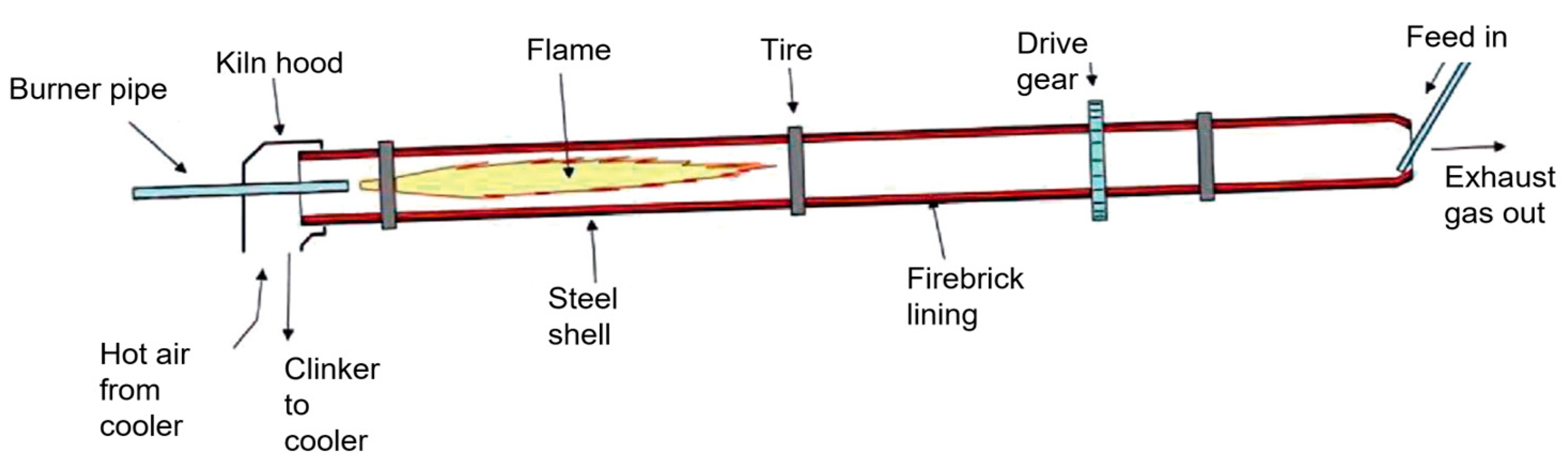
In a rotating kiln, clinker is produced and used for Portland cement [17]. This device basically consists of a large cylinder that spins once every one to two minutes around its axis. The lower end of this axis, which is inclined, is where the burner is situated. Following precalcination, the kiln is fed with the raw material. As it rotates, the feed is fed at the top of a preheat tower which flows slowly down as hot gases flow upward and then enter the kiln. Figure 2 depicts a revolving kiln’s general design [18].
Powdered feed is transported to the preheater as the first step of the pyro-processing unit once it has reached the desired composition and size. Here, a sequence of countercurrent flue gases from the calciner are used to preheat the raw materials. When the temperature reaches around 550 °C during preheating, limestone, and magnesium carbonate decompose, releasing CaCO3, MgO, and CO2. This is when the precalcination process is initiated in the preheat tower. Limestone’s (CaCO3) chemical breakdown into lime (CaO) and carbon dioxide (CaCO3 ⇌ CaO + CO2) begins in the precalciner. Table 2 is a list of the physical and chemical reactions involved in making cement. The preheat tower unit calcines about 90% of the raw feed. The precalciner system uses solid-gas heat exchange to produce direct combustion and spread and suspend raw grain cement in an airflow. The already-heated materials move to raise the temperature using the calciner even further before entering the kiln. In the revolving kiln, the precalcined meal undergoes the remaining calcination. Before being completed at 960 °C in the kiln, these processes continue in the calciner [
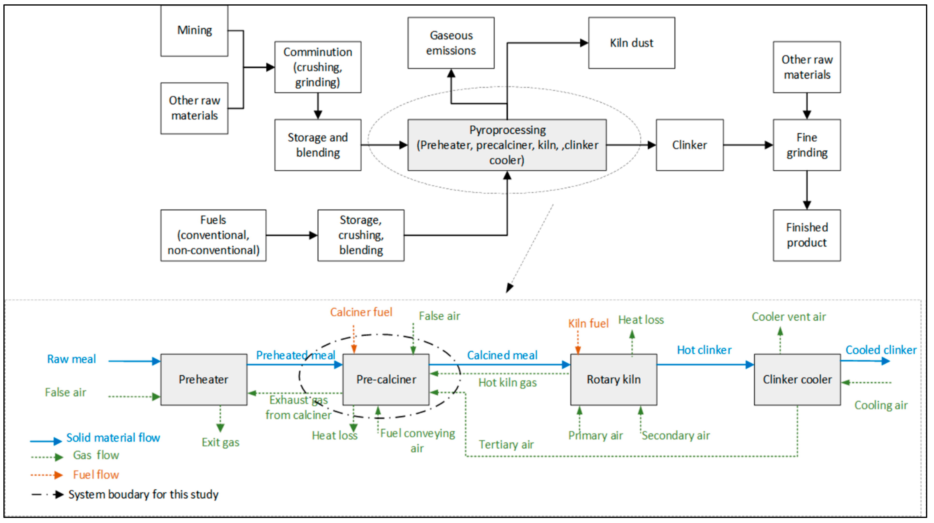
19]. The kiln facilitates numerous other physical and chemical processes in addition to generating cement. An illustration of a typical dry-based cement production facility is shown in Figure 3. There is typically a precalciner system in place between the rotary kiln and the preheater in modern cement-producing facilities. The final product from the kiln is called clinker. Clinker is a term used in the cement industry to refer to the hard, nodular material that is produced after cooling of the product generated from the kiln. C2S, one of the clinker’s constituents produced between 900 and 1200 °C, and other components including C3S, C3A, and C4AF are created between 1200 and 1280 °C in the kiln during the different phases of reactions [14]. Solid clinker finally melts at temperatures above 1280 °C to create a well-mixed and nodular clinker [19].
After cooling the clinker over the cooler stage with outside air from 1450 °C to 100 °C, the clinker is then transferred to the final unit for grinding and mixing. The warm air from the coolers is used in the calciner and the kiln, and the extra air is vented into the atmosphere. The heated air stream provides some of the kiln’s required heat energy as well as acting as an air source for the combustion process. The calciner is then supplied with the hot air stream from the coolers and kiln exhaust. Both of these streams act as a heat source for the breakdown of limestone and magnesium carbonate as well as a source of air for the combustion process [20]. The use of calciner exhaust to preheat input materials in the preheater step is the process’ main source of heat loss. According to [21], the preheater, calciner, kiln, and cooler processes, generally known as the pyro-processing unit, are considered the core of the cement manufacturing process and account for around 90% of the total energy required for cement production.
In the precalciner, the exothermic activity of fuel burning coexists with the endothermic process of the uncooked meal’s carbonate breakdown. When the precalciner is working at its best, energy is conserved and rotary kiln and precalciner emissions are reduced. The temperature inside the calciner, the amount of time the raw meal is allowed to remain in the system, solid gas separation, the impact of dust circulation, and the kinetic behavior of the raw materials are some of the factors that affect the precalciner’s efficiency [22]. The stability and effectiveness of the calcination process directly affect the final clinker quality, smooth operation in the subsequent rotary kiln operation, and the energy consumption of the pyro-processing unit.
Figure 3. Flow stream input/output information is shown in a schematic representation of a typical cement production facility for the pyro-processing phase [23].
Jmmp 07 00199 g003

2.3. Clinker Grinding into Final Product

Electrical fans are used to cool the hot clinker before it is transported to the grinding and blending mills. The last step in the process of manufacturing cement is clinker grinding. In this case, the clinker is powdered and mixed with additives. Depending on the availability of the additives, cement standards, and the cement market, specific amounts, types, and compositions of additives are added to the powdered clinker. From a technical and commercial perspective, the clinker factor (CF), or the proportion of clinker in cement, is an essential element.

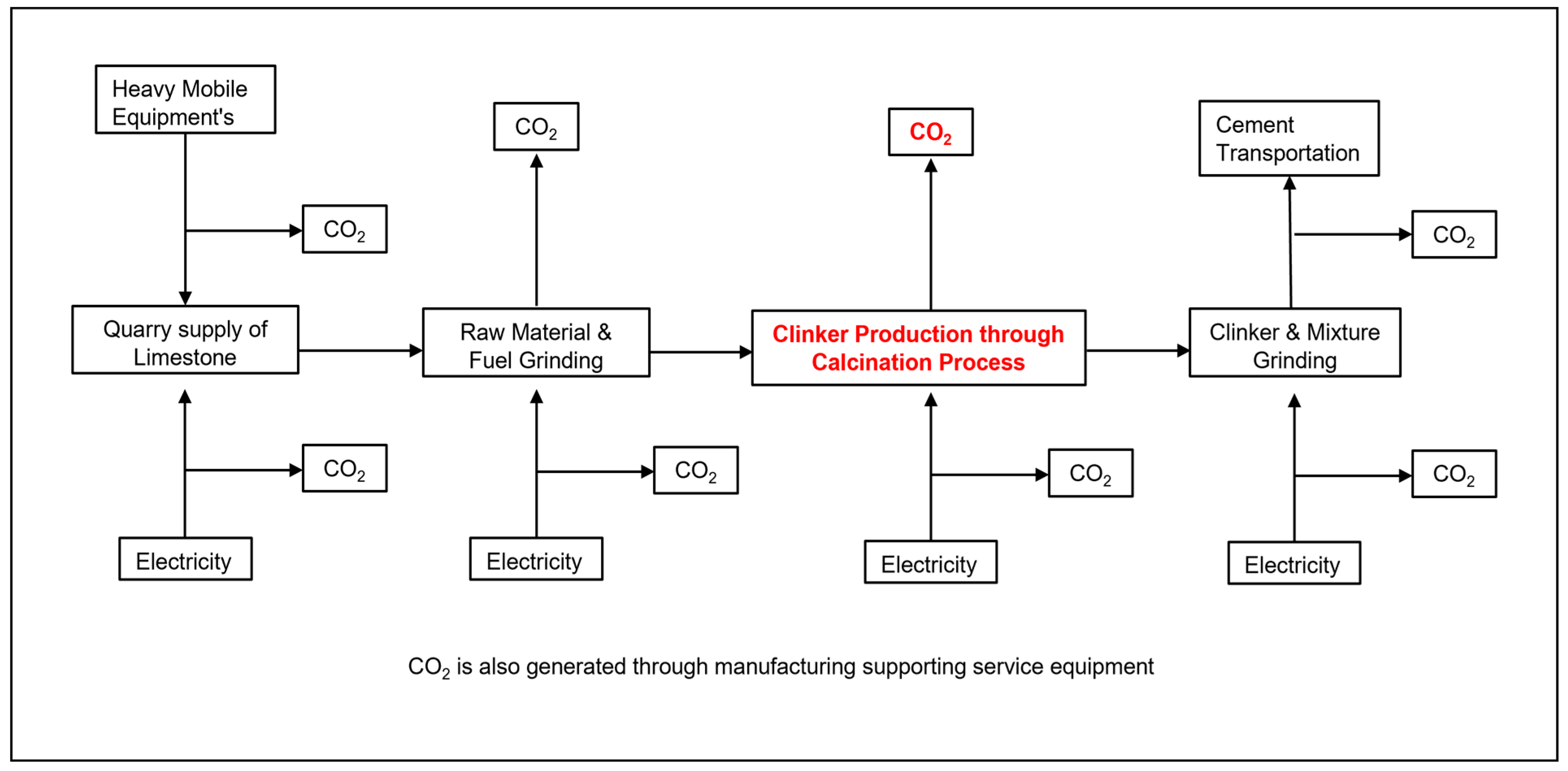
2.4. Calcination Process and CO2 Emission

Calcination is the heat process of driving off a volatile fraction that modifies the chemical makeup of mineral ore. Unlike pyrolysis, this process does not require the absence of oxygen [24]. Four sources contribute to the CO2 emissions during cement production: Transportation of raw materials accounts for 10% of total emissions, fossil fuel combustion during the calcination process generates 40%, CaCO3 and MgCO3 decomposition generates 50% of CO2 emissions, CaO and MgO are produced as the result of elementary chemical reactions, and electricity generated for electrical motors and facilities is responsible for another 10% [25]. Numerous large and minor technical and management concerns in the plant can affect plant performance and result in an increase in fuel and energy usage in addition to the intensive fuel utilization, power consumption, and basic chemical reactions mentioned above. These higher consumptions may result in substantial thermal waste and, as a result, extraordinary additional CO2 emissions. Figure 4 shows the various sources of CO2 in the cement manufacturing plant. As shown in Figure 4, our study focuses on CO2 generated through clinker production through the calcination process.
Carbonates decompose in a highly endothermic process [26]. A limestone particle must go through several phases of calcination, and each stage’s rate-determining factor is affected by the calcination circumstances. These processes involve heat transmission from the bulk gas to the particle’s exterior surface and from the external surface to the reaction interface, in addition to the chemical reaction that takes place at the reaction interface, and involve the mass transfer of carbon dioxide from the reaction interface to the bulk gas [27]. However, the rate of heat and mass transmission will frequently be high if the particles are small, and the bulk gas temperature is high. The process that determines the rate for the conditions in cement manufacturing is the chemical reaction [26,
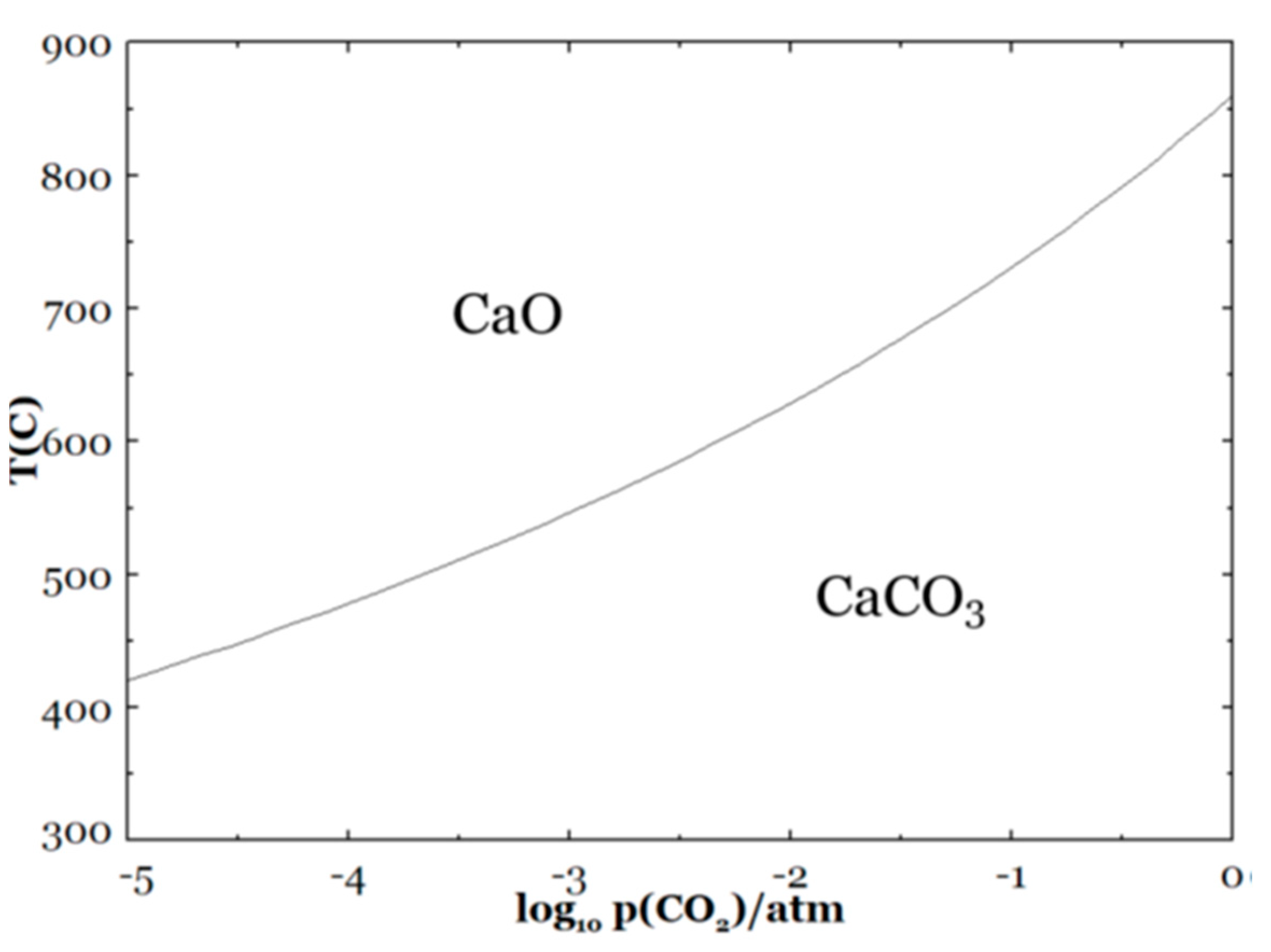
28]. By electrifying the calcination process, atmospheric carbon dioxide concentrations would increase from about 25 mol% to over 100 mol%. This could have an impact on a variety of elements as well as the process’ chemistry, heating of the raw materials, calcination, production of clinker, and final cooling. The rate of calcination will be slower due to the increasing partial pressure of carbon dioxide [29,30,31,32,33] and the increase in the required calcination temperature, as can be seen in Figure 5. Tokheim et al. [34] investigated the viability of an electrified calcination step and concluded that electrical heating-based calcination looks feasible and would offer comparable process parameters with no detrimental effects on product quality. A minor variation in the quality of the product was seen in laboratory testing on Oxyfuel combustion that modified the gas phase’s carbon dioxide content [35].
The kinetics and chemical mechanisms relating to the calcination of carbonates have been extensively discussed in other publications over the past few decades [37,38]; particularly, the calcination of CaCO3 (Takkinen et al. [39]), due to its technological significance. According to Garcia-Labiano et al. [40], there are several aspects of the reaction that are unclear. Considering the lack of agreement over the process, Reactions (4) through (6) have all been put forth.
CaCO3 (s) → CaO (s) + CO2 (g), ∆HR = +168 kJ/mol
CaCO3 (s) ↔ CaO* (s) + CO2 (g) ↔ CaO (𝑠) +CO2 (g)
CaCO3 (s) ↔ CaO (g) + CO2 (g) ↔ CaO (𝑠) + CO2 (g)
According to Hyatt et al. [38], CaO has a metastable structure. The active CaO, denoted by CaO* in Reaction (5), is thought to serve as a bridge between the newly formed CaO crystal and the unreacted CaCO3. Another strategy put up by L’vov et al. [41] is for CaCO3 to decompose into gaseous CaO and CO2 species while also condensing low-volatility CaO, as seen in Reaction (6) [41]. Regardless of the underlying source, calcination may be broken down into three stages: heating the particle surface and transferring heat there; chemical processes taking place at the reaction front; and the transfer of CO2 from the reaction front to the surrounding atmosphere. According to Stanmore and Gilot [37], the chemical makeup of the limestone, the size of its particles, the makeup of the surrounding gas, and the ambient temperature all have an impact on the reaction. This raises the level of uncertainty in the kinetic field.

2.5. Literature Review of Cement CO2 Emission Calculation and Prediction for the Cement Industry

For the sake of simplicity, a few imprecise approaches are widely recognized and frequently used to calculate CO2 emissions. There have been numerous estimates of CO2 emissions made in earlier studies. Calculating CO2 emissions requires several key metrics, including the carbon footprint. The term “carbon footprint”, also called “carbon profile”, is derived from the term “ecological footprint”, which was used to describe the total amount of carbon dioxide and other greenhouse gas emissions related to products, along their supply chains, and occasionally including their use, end-of-life recovery, and disposal [42,43,44]. In 1996, the IPCC published its first CO2 emissions factors related to cement manufacture, including a heat-processed lime-stone breakdown factor [45]. In addition, IPCC [8] provided the techniques and information required to calculate stationary combustion emissions in 2006. Three tiers of methodologies are provided for the sectoral approach based on data on fuel combustion from national energy statistics and fault emission factors, as well as data on fuel statistics and applied combustion technologies, as well as technology-specific emission factors. The default value recommended by the IPCC may either overestimate or underestimate the overall emissions of the Chinese cement sector, so it is crucial to properly estimate the process-related emission factor for clinker production together with accounting procedures. This emission factor can be determined based on the stoichiometric compositions of the reaction using the principal chemical processes in calcination, CaCO3CaO + CO2 and MgCO3MgO + CO2, as shown in Equation (7).
EFclinker =ContentCaO × 44/56 + ContentMgO × 40
where ContentCaO and ContentMgO indicate, based on plant-level assessments, the CaO and MgO contents of clinker that should be computed. In 2012, Shen et al. [46] examined the 289 production lines’ raw materials, raw meals, clinker, cement, and fuel throughout China’s 18 provinces. They calculated the process emission factors for each type of kiln, which are 1.4–3.4% lower than the IPCC Guidelines’ default values. Based on detailed information from 1574 cement companies in 2013, Cai et al. [47] without mentioning the particular amounts of CaO and MgO, estimated that the total process emission factor was set at 0.504 t CO2/t clinker. In 1994 and 2005, the UNFCCC and NDRC estimated the process-related emissions to be 157.8 Mt CO2 and 411.7 Mt CO2, respectively [48,49]. High variances and uncertainty in energy consumption are other problems, as the amounts of coal used to heat the kiln were calculated by varying stated coal intensities rather than those immediately available in the official figures [50]. Lui et al. [50] demonstrated another equation used to calculate CO2 emission in cement manufacturing plants. This unit-level process and fuel-based CO2 emissions are estimated using the following Equation (1):
Ei = Pi × Rk,i × EFprocess,k + Fi × EFcombustion,k
where, respectively, i and k stand for the unit and the nation; P stands for cement production (t), R for the clinker-to-cement ratio, F for fuel consumption (kJ), EFprocess for process-based emission factors (g/kg), and EFcombustion for combustion-based emission factors (g/J). E stands for unit-based emissions (kg); P for cement production (t); R for clinker-to-cement ratio; and F for fuel consumption (kJ). It should be emphasized that this study only measures the emissions that directly result from the manufacturing of cement; indirect emissions, such as those from the use of gasoline in power plants to generate electricity and the fuel used by vehicles to transport materials, are not considered [50].
It is noticeable that IoT, Artificial Intelligence (AI), machine learning (ML), real-time monitoring, and optimization techniques are considered some of the emerging practices that are reshaping the world and how research is performed. As mentioned, most of the methodologies mentioned herein are based on the calculation of CO2 emission quantity by empirical methods, but Van Gio et al. [51] performed an extensive investigation on leveraging machine learning techniques for high-precision predictive modeling of CO2 emissions. They show that predictive analytics utilizing machine learning algorithms play a pivotal role in various domains, including the profiling of carbon dioxide (CO2) emissions in innovating ways to understand CO2 emission. The study shows how these algorithms are useful for quantifying emissions, evaluating energy sources, improving prediction accuracy, and accurately estimating CO2 emissions. In particular, deep learning, artificial neural networks (ANN), and support vector machines (SVM) demonstrate effectiveness in a range of industries, and the Modified Regularized Fast Orthogonal-Extreme Learning Machine (MRFO-ELM) algorithm optimizes predictions pertaining to coal chemical emissions.
Many articles have discussed the use of cutting-edge technologies, such as artificial intelligence (AI) and machine learning (ML), to reduce carbon emissions [52,53]. Using the ARIMA technique, Yang and O’Connell [54] provided an emission projection for the fuel consumption in air travel over a five-year period for the Chinese aviation industry. Niu et al. [55] provided a case study on how to use machine learning algorithms in conjunction with an algorithm combination approach to predict carbon emissions by 2030. Using data from 2015 to 2019, Javadi et al. [56] conducted a study whereby they utilized the RBF network model to predict the amount of greenhouse gas emissions in the Iranian vehicle sector by 2030. Olanrewaju et al. [57] also used the ANN algorithm to predict emissions in their study on the management of emissions in Canada’s industrial sectors, specifically for the year 2035. Several machine learning (ML) algorithms, including RF, LSTM, SVM, and others, were used to forecast N2O emissions in agriculture in a different study by Hamrani et al. [58], and the results were assessed for predictive accuracy. Additionally, the LSTM, CNN, and KNN algorithms were used both singly and in combination to predict air pollution in order to control and lessen its adverse effects [59]. It should be mentioned that although the research used ANN, SVM, and deep learning algorithms to estimate Flu-Gas emission [60], five predictive accuracy criteria were used to assess the methods’ accuracy.
Even though many studies cited herein show how the adoption of machine learning and AI is being used to successfully predict CO2, this is not the same for the cement manufacturing industry. Boakye et al. [61] show why machine learning and AI are not well adopted in the cement, aggregate, and concrete industries. Literature searches find only a single study that describes using machine learning to predict CO2 based on calcination. Unfortunately, the study does not use manufacturing performance data but is based on laboratory experimental data. Lei et al. [62] reported other empirical methodologies used to estimate the amount of CO2 emission from cement in addition to these well-known ones, but this study employs machine learning to forecast CO2 emissions using laboratory data. The paper noted that testing the models used by selected process data that represent extreme and typical plant operation conditions is recommended. This will lead to the development of more realistic models based on the actual plant data. This current paper employs machine learning and AI concepts using historical cement manufacturing real plant performance monitoring data gathered through instrumentation to predict CO2. This will establish the need to adopt innovative technologies in the cement manufacturing industries to help better understand CO2 emission and prediction.

3. Materials and Methods

Examining certain circumstances or events in detail is necessary to produce reliable projections. Even while the number of datasets available will increase as sensing capabilities advance, offering unmatched insights into process conditions, this makes the development of specialized big data analytics tools necessary to maximize the value from such data. The quantity and features of input elements that manufacturing organizations transform into output factors can be used to distinguish them from one another. When dealing with such intricate non-linear systems, modeling is helpful. Several academics have attempted to identify correlations between the variables in the precalciner process using the soft and hard modeling technique. Mass and energy balance (MEB) is a key technique for determining correlation and selecting the required process output. When the input parameters for the MEB computation are uncertain or impossible to measure directly, an iterative procedure is used. An alternative MEB approach is illustrated by machine learning techniques, which omit this iterative phase. Recently, data mining and machine learning methods have been extensively applied in predictive analytics. However, they are comparatively underutilized in prescriptive analytics. According to our research, only one study fully utilizes machine learning and data mining techniques to forecast CO2; however, the model’s data are entirely derived from experimental data rather than actual process manufacturing data [63]. Because most cement production companies have very strong data protection laws that forbid the public from processing historical data, it is necessary to rely on lab data. Since the primary author works in the cement sector and has access to this dataset, this study is a unique instance. The approach used for this study is described below, and it is crucial to highlight that this work is exclusive to this cement factory. The goal is to demonstrate that machine learning technologies may be used to anticipate the amount of CO2 emissions and to offer recommendations for how this discovery is essential to long-term sustainability solutions for the cement industry.
In modeling/nonlinear industrial processes that deal with noisy, constrained, and nonintegrated data, machine learning (ML) has demonstrated promising outcomes. Artificial neural networks (ANN) and support vector machines (SVM) are two examples of machine learning techniques that have demonstrated their efficacy in this area. For calculating the apparent degree of calcination, Gang and Hui [64] created a model utilizing a least Squares support vector radial basis function (RBF) kerneled machine (LSSVM). The temperature and pressure of the furnace, the calciner’s outlet temperature and pressure, the temperature of the tertiary air, and the quantity of cement raw that was laid off were all inputs into the model. To stabilize the precalcination process while achieving the necessary amount of precalcination of the raw food, low carbon monoxide, and considering the precalciner system’s multivariable dependency Griparis et al. [65] developed adaptive, resilient, and fuzzy control. Using five factor, coal flow to the kiln, coal flow to the precalciner, raw meal flow, the kiln’s rotating speed, and the negative pressure at the preheater exit, we may estimate the kiln’s temperature and oxygen content. Yang et al. [66] developed a back-propagation neural network (BPNN) and radial basis function neural network (RBFNN). The effectiveness of the machine-learning algorithms is strongly influenced by the quality of the input data. Gathering and preparing the training dataset is, therefore, an essential step in the modeling process. Simulated data, data from actual processes, and data from tailored experiments are all acceptable forms of training data. Simulated data is produced by theoretical models, including statistical models and computer simulations. Many industrial organizations have historical data in their systems, and the real process data are raw process data that were randomly selected. This study looks at using industrial historical data. A Taguchi or Design of Experiment (DOE) approach can be used to obtain designed experimental data. This study aims to improve the understanding of the generation of CO2 during cement manufacturing by dissection of the manufacturing processes using thousands of plant health data points from various installed measurement instrumentations. Modeling the calcination process in cement using machine learning algorithms with historical manufacturing process data will be new. This will be a novel attempt to find commonality in these large datasets with separately calculated CO2 emissions.
The step-by-step system structure for the research work of machine learning (ML) predictive analytics of the calcination CO2 generation is shown in the process flow model (Figure 6). Sensitivity analysis uses historical manufacturing health data from over ten thousand input variables, and the results are used to train the algorithms.
Like linear regression models, the method of maximum likelihood or the least squares approach is widely used to calculate a nonlinear regression model’s parameter. The parameter estimates from both estimating procedures are equivalent when the error components have a normal distribution and a constant variance. Nonlinear regression models usually never offer mathematical formulations for the maximum likelihood and least squares estimators, in contrast to linear regression models. These calculations are frequently only accessible through linear regression. Both estimation methodologies, however, necessitate the use of time-consuming numerical search techniques. Therefore, it is usual practice to evaluate nonlinear regression models using standard computer software tools. The utilized nonlinear regression model is shown in Equation (9).
F C t = α 1 exp ( b 1 N P c C ) + α 2 exp ( b 2 S F C ) + α 1 exp ( b 3 N P s C )
Various regression models are analyzed and based on these findings; the models are used to identify which cement manufacturing independent variables had the biggest impact on the dependent variables; that is, which will yield the lowest root mean squared error (RMSE). The suggested models’ accuracy was assessed using the following metrics: something which determines coefficient (R2) (Equation (10)), RMSE, Equation (11), the Durbin–Watson test (Equation (12)), the F-test, and the t-test.
R 2 = 1 ( r e s i d u a l s ) 2 ( P r e d i c t e d V a l u e s ) 2
R M S E = 1 m i = 1 m ( y i y ^ i ) 2
N is the number of datasets, and y and y are the laboratory measurements and their corresponding estimated values using the suggested model. A model with a lower RMSE would, if applied, have a lower overall error rate and more predictive power. To determine whether multi-collinearity is present, the Durbin-Watson statistic is utilized. The Durbin-Watson distribution’s magnitude values range from 0 to 4, and the number 2 in the middle denotes the absence of any correlation between the variables entered [67]. A number between 1.5 and 2.5 is sufficient to produce multicollinearity-free models. The Durbin-Watson, or DW, statistics (Dahish et al. [68]) are calculated using Equation (12) herein after.
D W = t = 2 T ( e t e t 1 ) t = 1 T e t 2
Users of mathematical and simulation models can analyze how each model input affects the outcome using sensitivity analysis to understand how the model output is dependent on the input. Python coding analysis was selected for this work. To identify which independent variable has the biggest impact on CO2 emissions, the significance of the independent variables will also be assessed. The Artificial Neural Network (ANN) model’s hidden layers and number of neurons were chosen at random. The design of an ANN network representing inputs and outputs is shown in Figure 6. An artificial neural network makes up the neural network. These skills are made possible by the circuit’s inclusion of elements that take cues from the biological similarities of the neurons to enable the learned neurons’ ability to detect solutions, formulate predictions, characterize data, and even foresee future events. As a result, numerous applications were found in the modeling of numerous forecasts for concrete strength blends as well as the simulation of extremely complicated interactions. A network of this type, however, typically consists of several layers with different sequential ordering, each of which includes a group of neurons connected to the neurons in the layer(s) above it in a similar way. We use actual input and output data for the first and last layers, which are the input and output variables. The hidden layers are typically thought of as multi-layered structures that use the input data to modify the hidden data. Using learning principles and neural networks, neuron weights can be adjusted to improve network emulation or task performance until a system satisfies the requirements for emulation or accomplishes its objectives. The input-to-output transformation of each neuron is applied to the data in the case of neuron transfer functions, which are now referred to as mathematical functions. The back-propagation method is particularly useful when using the log-sigmoid transfer function, which is extensively used in hidden layer neurons. In order to translate inputs into their corresponding outputs, the hidden (transitional) and output layers must go through two separate phases. A constant factor is multiplied by the sum of a neuron’s input and weight to determine its net input. Creating the product from the net input is the second step. The new multi-layer feedforward neural network design shown in Figure 7 consists of one output neuron, eight input neurons, six hidden neurons in the first layer, and four hidden neurons in the second layer. A fundamental type of neural network called the multi-layered perceptron (MLP) comprises three layers of neurons: input, hidden, and output, as well as forward information flows (Figure 7). Feedforward backpropagation (FFBP), the resulting network, involves applying the steepest or gradient descent approach to reduce the error value between realized and desired outputs. In other words, the weight correction (W) is proportional to the rate of global error change (E) with respect to that weight, according to Equation (13).
Δ w a E w
After examining various network topologies, FFBP will advise the number of hidden layers and the overall number of nodes in the input and hidden layers. There are several ways to prevent overfitting in ANNs. Giustolisi and Laucelli [69] summarize these strategies.

Source of Data in Cement Manufacturing

Understanding the performance of all assets and processes at a cement plant requires that digitization is adopted. Sensors and instrumentation should ideally be installed along assets to measure performance by converting analog to digital. These digital data can then be stored to track real-time performance trends that decisions can be based on. Figure 8 shows a typical digitization workflow process for cement manufacturing plants including Programmable Logic Controllers (PLC).
The data were chosen for 3 years of measurements from various sensors placed throughout the manufacturing facility. These sensors were chosen based upon their likelihood to contribute more significantly to CO2 generation than others. Days that produced null measurements where measurements were expected were removed from the dataset. The dataset was then normalized for better comparison.

4. Results

Feature correlation heat maps were first used to narrow the scope of our research by establishing potential correlation and eliminating those variables with little to no relevance in terms of CO2 generation (dimensionality reduction). Predictive models were then generated using the string potential correlation input variables. Presented herein are the results obtained for the different sections of the production line as mentioned in Section 2 of this paper. In addition, predictive model results are also presented herein. More than 60 independent input variables containing over 50,000 data points were used for sensitivity analysis. The dataset was divided 80/20 to train and test the quality of the model used. One limitation to the model was that key manufacturing sensors were used and compared to CO2 calculations for each day. The model is only comparing manufacturing processes that had sensors, so it is possible that other non-measured sources could contribute to the CO2 generation. Additionally, while largely reliable, sensor readings could also introduce some level of error in measurements. But in general, they result in a high level of reliability of the dataset. The independent variables in cement manufacturing were selected because they are all the performance tracking instrumentation sensors associated with the calcination process phases with the preheat tower and kiln that most likely contributed to CO2 generation. Figure 9 shows the workflow of proposed ML techniques used for analysis.

4.1. Preheat Tower Data Analysis

To better understand how the process variables impact the emission of the CO2, predictive tools were adopted. Results for the Python analysis are reported herein. Thirty-one independent preheating input variables containing over 31,465 data points were used for sensitivity analysis against CO2. The data for this analysis covers the operations from 1 January 2020, through 23 October 2022. Table 3 shows the statistical analysis of the dataset analysis. Figure 10 shows a typical Python code used for the heat map model.
Feature correlation heat maps were first used to narrow the scope of our research by establishing potential correlation and eliminating those variables with little to no relevance in terms of CO2 generation. The datasets run showed the strongest correlations among the two cement manufacturing processes. Figure 11 shows the heat map of the sensitivity analysis performed. Similar Python coding was used for the analysis. The heat map is the local sensitivity analysis results for the final model using manufacturing real-time instrumentation process historic data of the preheat tower system as input variables against output data of CO2. It presents the sensitivity indices of cement manufacturing process metrics for the most sensitive parameters across the preheater system. Sensitivity indices represent the relative change in the metric that results from changing parameter values. The intensity of the color in each panel correlates with the magnitude of the parameter sensitivity, with deep blue representing a positive correlation between the parameter and lighter blue representing a negative correlation. Table 4 shows the variables’ description of the heat map.
Examine quantitative survey data to find significant patterns, trends, or linkages between the variables. The correlation is shown in Figure 12. Figure 12 shows the PREHEAT.STG.3 CYCLONE GAS OUTLET TEMP. [0–900 [°C]] as the variable which has the highest correlation R2 with the CO2.
The dataset was used to train five categories of regression models. The model with the lowest RMSE for each category was chosen to forecast the three outcome variables of apparent calcination degree and CO2 molar fraction. Also displayed are the ANNmodel outcomes. To demonstrate how the conventional linear regression method differs from other approaches, it also displays the results of the linear regression classical model. Figure 13 below shows the predictive modeling of the dataset using multiple regression analysis. The results are represented herein.
Root mean square error (RMSE), commonly referred to as root mean square deviation, is one of the most widely used techniques for evaluating the precision of forecasts. It demonstrates the Euclidean separation between forecasts and observed true values. The RMSE indicator shows how closely the obtained data are clustered around the predicted values, indicating how dispersed these residuals are. The RMSE decreases as the data points get nearer to the regression line because the model has less error. The RMSE for the linear, ridge, decision, and random regression are all equal to or below 0.05. The Lasso regression analysis is 0.24. Predictions made by a model with lower error are more accurate. RMSE values use the same units as the dependent (outcome) variable and have a range of zero to positive infinity. Figure 14 shows the RMSE with different algorithms for the predictive modeling.

4.2. Kiln Data Analysis

As mentioned in the context of this paper, the final stage of the calcination process happens in the kiln. The kiln dataset used for this analysis covers the kiln inlet through the kiln and the kiln outlet. The dataset comprises the rotary kiln inlet O2 of about 6.39% with oxygen 3106 PPMsw. The temperature ranges from 1100 °C at the kiln inlet to 1600 °C at the burning zone of the kiln. The gas flow rate inside the kiln determines how quickly fuel burns and how long solids stay there. In calciner systems with tertiary air flow, the calculated gas duration ranges from 1.4 to 1.7 s to 4 to 5 s in total or hybrid flow systems, depending on the size of the kiln. The kiln system has multiple instrumentations installed for monitoring the processes and controlling the processes which allow this dataset to be collected. These monitoring instruments measure variables such as gas temperatures, pressure drops, material temperatures, fuel flow, heat inputs, kiln feed rate, clinker production rate, drivers’ power, oxygen flow, etc., which are compiled as a dataset. This dataset is stored in the historical database and was extracted for this analysis. Note that the manufacturing process is managed using multiple control loops. A multivariable process called a kiln has intricate interactions between its various factors. It is more coupled, exhibits strong nonlinearities, and experiences frequent disturbances. The dataset of all the complex variables is extracted into Excel format and used for this analysis.
Note that this dataset does not include the cooler since there is no calcination process that takes place during the cooling. Twenty-one independent kiln input variables containing over 21,315 data points were used for sensitivity analysis against CO2. The data for this analysis covers the operations from 1 January 2020, through 23 October 2022. Results for the Python analysis are reported herein. Table 5 shows the statistical analysis of the dataset analysis.
The datasets run showed the strongest correlations among the cement manufacturing process. Figure 15 shows the heat map of the sensitivity analysis performed, providing data visualization of the correlation of these manufacturing processes to the calculated generation of CO2 for the process. Heat map of the local sensitivity analysis results for the final model using manufacturing real-time instrumentation process historic data of the kiln entire system as input variables against output data of CO2. As depicted by the feature correlation heat map below, V15 (Kiln Main Drive Control Speed) had the highest correlation with the amount of CO2 generated during the final stage of the calcination process. Table 6 shows the variables’ description of the heat map.
Examine the quantitative survey data to find notable patterns, trends, or linkages between the variables as shown in Figure 16. The KILN MAIN DRIVE SPEED CONTROL [0–100%] is the variable which has the highest correlation R2 with the CO2. The kiln main drive speed is normally about 4.50 RPM. This means that the kiln speed has influence on the calcination degree and can be used as a predictor of the amount of calcination degree through the cement manufacturing process.
The dataset was used to train five different regression model types. The model that provided the lowest RMSE for each category was chosen to forecast the output variables of apparent calcination degree and CO2 molar fraction. Figure 17 below shows the predictive modeling of the dataset using multiple regression analysis.
The RMSE for the linear, ridge, decision, and random regression are all equal to or below 0.05. The Lasso regression analysis is 0.24. Predictions made by a model with lower error are more accurate. RMSE values use the same units as the dependent (outcome) variable and have a range of zero to positive infinity. Figure 18 shows the RMSE with different algorithms for the predictive modeling.

4.3. Preheat Tower and Kiln Systems

The combined system which included the preheat tower and the kiln dataset was considered. Results for the Python analysis are reported herein. Table 7 shows the statistical analysis of the dataset analysis of the correlation coefficient between the two highest systems.
Feature correlation heat maps were first used to narrow the scope of our research by establishing potential correlation and eliminating those variables with little to no relevance in terms of CO2 generation. The datasets run showed the highest correlations among the cement manufacturing process. Heat map of the local sensitivity analysis results for the final model using manufacturing real-time instrumentation process historic data of the kiln entire system as input variables against output data of CO2 (Figure 19). Upon narrowing the results of both the preheat tower and the kiln systems, a Pearson correlation was performed to evaluate the linear relationships between each measurement and the corresponding CO2 calculated over the same time frames (Equation (14)).
r = ( x i x a v e r a g e ) ( y i y a v e r a g e ) ( x i x a v e r a g e ) 2 ( y i y a v e r a g e ) 2
The highest yielding outputs from both the previous kiln and preheat analyses were then compared to produce the highest overall correlation of the dimensionality-reduced set of features using multivariate regression. Figure 20 shows the KILN MAIN DRIVE SPEED CONTROL as the variable which has the highest correlation R2 with the CO2. The pressure daft at stage 5 is −19 mBar and at stage 1 are draft −81 mBar. In consideration of all the system data, the correlation shows that the draft pressure in the preheat tower at stage 1 is the most critical to the predictability of the calcination process and emission of the CO2.
Figure 20 below shows the feature of importance of the dataset using multiple regression analysis. V2 and V15 can be referenced to Table 4 and Table 6.

5. Discussion

One of the most significant environmental challenges that our civilization is currently facing is the threat posed by climate change. One of the main greenhouse gases is carbon dioxide (CO2). The objective of the current study is to identify the variables that have a greater overall impact on CO2 emissions during the cement production process. The two primary chemical processes in a Portland cement manufacturing facility are calcination and clinker reactions, which ordinarily take place in the cement calciner and rotary kiln, respectively. The most energy-consuming step in the cement manufacturing process, calcination, produces CO2 as a byproduct. An explanation of the analysis output follows.

5.1. Current Trend of Dealing with CO2 Emission in the Cement Industry

As stated in the article, around 8% of global carbon dioxide emission, is caused by the cement sector. The cement industry is now examining a wide range of options to lower the CO2 emissions footprint of cement production and help the global cement industry achieve the roadmap vision pathway. As mentioned in the International Energy Agency (2018) study, the cement manufacturing industry is adopting several strategies to help achieve NetZero CO2 emissions by the year 2050. It is significant to highlight that the paper’s findings play a crucial role in identifying these routes and suggest strategies for utilizing machine learning to advance this objective. Artificial intelligence and machine learning are now essential components of modern life, and they have helped to demonstrate the presence of humanity in several ways. Unfortunately, machine learning and artificial intelligence have not been fully utilized in the cement manufacturing industry to understand how things might be improved. Here are some of the ways the cement industry is attempting to reduce CO2 emissions and how this study’s innovative findings contribute to achieving the goal:
  • By incorporating cutting-edge technology into brand-new cement plants and upgrading existing facilities to achieve higher energy performance levels where practical from an economic standpoint, we can increase energy efficiency. According to the International Energy Agency, increasing energy efficiency in cement production will result in 0.26 GtCO2 or 3% less CO2 emissions globally in the 2DS compared to the RTS by 2050. This equates to 12% of the worldwide cement industry’s current direct CO2 emissions. The energy required to burn cement clinker (about 1700–1800 MJ/t) and the heat required for drying and preheating raw materials together makes up the potential amount of thermal energy required to generate cement clinker;
  • Coal is the fuel that is most frequently used, accounting for 70% of the thermal energy used globally to manufacture cement. Together, oil and natural gas make up 24% of the thermal energy required to produce cement globally, while biomass and waste (alternative fuels) make up a little over 5%. To balance the use of carbon-intensive fossil fuels by using biomass and waste materials as fuels in cement kilns in place of conventional fuels to reduce carbon emission biogenic and non-biogenic waste streams that would otherwise be inappropriately disposed of, burned, or transferred to landfills are referred to as “wastes” in this context and can be used as alternative fuels. By using alternative fuels instead of conventional fuels, we can reduce our carbon footprint; the world’s CO2 emissions will be reduced by 0.9 GtCO2, or 12%, by 2050 as compared to the RTS. This equates to 42% of the direct CO2 emissions that the worldwide cement sector now produces;
  • Increasing the use of blended ingredients substitutes and expands the market for blended cements, and will help to lower the quantity of clinker needed per ton of cement or every cubic meter of concrete produced. By 2050, lowering the clinker to cement ratio will cut world CO2 emissions by 2.9 GtCO2, or 37%. This is equivalent to 128% of current direct CO2 emissions of global cement production. Fly ash (Type C and Type F), slag cement, and to a lesser extent silica fume are the SCMs most frequently employed in concrete formulations. These materials are leftovers from several industries: Power stations burn coal with fly ash; iron ore is smelted with slag cement; and silicon or ferrosilicon is alloyed with silica fume. Recent years have seen a lot of research on alternative materials, like biochar, that can be utilized as SCM for carbon capture and sequestration in concrete;
  • Using emerging and innovative technologies that:
    By using energy storage and distribution systems like EHR technology to generate electricity from thermal energy that would otherwise be wasted, the cement industry may assist in the adoption of renewable-based power generation technologies like solar thermal power and contribute to the decarbonization of electricity generation. As a clean energy source, hydrogen has also been investigated.
    Carbon Capture systems in the cement-making process for long-term sequestration or storage are currently being explored. A new method called carbon capture, utilization, and storage (CCUS) has the potential to lower greenhouse gas emissions from the manufacture of cement. A reasonably pure stream of carbon dioxide from industrial sources is isolated, processed, and then delivered to a place for long-term storage as part of the carbon capture and storage process. The carbon dioxide stream that needs to be caught, for instance, may be produced by burning biomass or fossil fuels. Over the next ten years, advances in technology and legislation are expected to raise the quantity of CO2 gathered by 800 MT. Through 2050, 70–100 projects will be required annually to handle this scale-up. Rapid adoption of the ready-now technology will be required to get there.
The creation of low-energy cement with a smaller carbon footprint is another creative discovery to aid in the reduction of CO2 generation in the cement manufacturing process. Izadifar et al. [70] showed in their study that using cement clinkers predominantly constituted of belite (β-C2S as a model crystal), which replaces alite, is an environmentally beneficial strategy to minimize the high level of CO2 emissions in Portland cement production. Their research demonstrates that variations exist in the previously stated dissolution timeframes for both perfect and imperfect crystals, which are caused by the statistical properties of the KMC algorithm as determined by executing ten numerical realizations. The study finds that it is feasible to analyze the various dissolution behaviors of the individual facets of belite crystals by upscaling atomistic models, and that this could eventually result in the manufacturing of more reactive belites that could be used to make Portland cement clinker. Cement manufacturing efficiency can be crucial in understanding CO2 in production and in assisting with CO2 reduction efforts. To produce consistently high-quality products, which is the purpose of clinker manufacturing, several variables must be under control. Understanding the impact of these factors’ variation on the chemical reactions occurring during the process is necessary. The control of these variables can aid in reducing emissions if the amount of CO2 from the manufacturing stream can be predicted. The bulk of estimations for CO2 for cement plants, according to the literature analysis for this paper, are based on the quantity of clinker produced and the type of thermal energy source multiplied by a factor. Our study makes use of machine learning to identify the process variable that has the greatest impact on CO2 emission and to forecast CO2 emission utilizing these factors. This study’s results section demonstrates that two variables are essential to the pyro-system of the manufacturing process. The investigation took historical manufacturing data into account. First, PRE-HEAT.STG.3 CYCLONE GAS OUTLET TEMP. [0–900 [°C]] is one of the two variables, along (2) CONTROL FOR KILN MAIN DRIVE SPEED. These two factors are thoroughly explored here.

5.2. Preheat.STG.3 Cyclone Gas Outlet Temp. [0–900 [°C]]

The calcination of the limestone blend begins in the preheater cyclone stages, as was already described. This section justifies the reason why the preheat temperature makes sense with the correlation. In many situations, temperature can significantly affect CO2 emissions. Increased CO2 emissions may occur from more complete burning of fossil fuels at higher temperatures. These processes can proceed more quickly at higher temperatures, increasing emissions. At normal pressure, limestone decomposes at a temperature of 898 °C, and once the temperature exceeds 925 °C, it breaks down quickly. Only when the temperature rises above the temperature at which the carbonates in limestone dissociate, which is normally between 780 and 1340 degrees Celsius, does the reaction start. Agglomeration and shrinking increase with temperature.
The CO2 that is evolved during the process must be eliminated, and the temperature must be kept above the dissociation point. The CaCO3 eventually dissociates from the particle’s outer surface inward, leaving behind the desired CaO layer. As a result, the procedure is dependent on a sufficient fire temperature of at least 800 degrees Celsius to enable decomposition and a decent residence time or holding the lime or limestone at temperatures of 1000 to 1200 degrees Celsius for an acceptable amount of time to manage its reactivity. The elements that affect calcination are the limestone’s crystalline structure, internal strength, and the size of the crystals that form following calcination. Smaller crystals unite to form larger crystals during calcination, which causes the larger crystals to contract and lose volume.
Higher agglomeration and more shrinkage result from calcination at higher temperatures. In addition, the crystal structure of limestone is connected to its density. The void space between crystals is determined by the crystal form, which also affects the density of the limestone. Volume is reduced during calcination because larger voids make it easier for CO2 gases to pass through. Some limestones dissolve during the calcination process because of their crystalline structure. Limestone of this kind is not suitable for calcining. Another limestone exhibits the exact opposite behavior. This sort of limestone is calcined until it becomes so dense that CO2 cannot escape, and it becomes nonporous.
The substance’s reactivity is used to gauge how quickly lime responds in the presence of water. To find out how reactive ground lime is, a test process involves slaking it in water. Numerous procedures and factors relating to the raw materials have an impact on the reactivity of lime. These factors include (i) the burning temperature and duration, (ii) the crystal structure of the limestone, (iii) impurities, and (iv) the type of fuel and kiln. According to how reactive it is, lime is typically divided into four categories: (i) dead burned, (ii) hard, (iii) medium, and (iv) soft. Fewer reactions of lime is frequently described as being medium, hard, or dead burned. The limestone used as fuel and feedstock has an impact on the properties of lime as well. For instance, coke-fired shaft kilns often produce lime with a medium to low reactivity, but gas-fired parallel flow regenerative kilns frequently produce a high-reactivity lime. The primary factors influencing lime’s utilization are its chemistry and reactivity. In the instance of the Union Bridge Plant, the process raises the temperature in the preheat tower using coal as a thermal fuel source. The coal also has carbonate compounds, which are burned to produce the high temperature in the preheat tower and emit carbon dioxide (CO2).
Dolomite and dolomitic limestone deterioration is considerably more difficult. One, two, or even more distinct stages, as well as transitional ones, might be involved in decomposition. The reactions involved in these phases are CaCO3.MgCO3 + heat = CaCO3.MgO + CO2, CaCO3.MgO + heat = CaO.MgO + CO2, and CaCO3.MgCO3 + heat = CaO.MgO + 2CO2. Dolomite and dolomitic limestone require temperatures between 500 and 750 degrees Celsius to decompose. Technologies for reducing CO2 emissions from industrial processes, such as carbon capture and storage, can perform better or worse depending on the temperature. Overall, warmer temperatures have the potential to worsen the issue of CO2 emissions and contribute to global warming, which has a variety of effects on the environment and society. As explained here and shown in the results, the degree of temperature in the preheat tower is directly correlated with the degree of calcination resulting in the amount of CO2 emission (Figure 11). The degree of temperature is correlated with the amount of total heat consumption. This clearly supports the results obtained by conducting sensitivity analysis and predictive analytics using machine learning tools. This, therefore, shows why there is a strong correlation depicted in the result section of temperature on stage 3 with CO2 emission.

5.3. Kiln Main Drive Speed Control

The kiln main drive speed control variable has the highest correlation with CO2 based on the sensitivity analysis. A kiln’s main drive speed, which is frequently linked to the drum or shell’s spinning speed, can have a direct impact on CO2 emissions. However, the link is intricate and is reliant on circumstances and processes. Why is the kiln main speed control having such an impact on the calcination process? The following outlined reasons explain the impact. An electric motor with a frequency converter, a gearbox, couplings, and an auxiliary drive make up the drive. Diesel engines can be used as auxiliary drives. The continuous process of raising materials to a high temperature (calcination) is carried out in a rotary kiln, which typically rotates at a speed of 1 to 3 rpm but can occasionally reach 5 rpm. The amount of calcination and reaction that takes place depends on how long materials remain within the kiln, which is affected by the main drive speed. Shorter residence times brought on by higher main drive speeds may have an impact on kiln fuel economy and clinker quality. The main driving speed can affect energy use and, consequently, CO2 emissions. The efficiency of calcination, which in turn influences the amount of energy used and emissions produced by these processes, is also affected by the main drive speed. The firing process may be impacted by the main drive speed, which could have an impact on emissions and energy use. The link is not linear, though, and important roles are also played by other variables such kiln design, fuel type, feed material composition, and process optimization. Some contemporary kilns have cutting-edge energy-saving and emission-reduction technology, which can lessen the effect of main drive speed on CO2 emissions. In actuality, the calcining zone and the maximum temperature in the traveling bed must be positioned in such a way that the coal has a reasonably long travel time as it completes calcination to achieve the desired provision of stable kiln operation. Effective calcination can be accomplished with the least amount of feed and, ideally, without the use of any additional fuel (more than 75%, or perhaps 85% or more of the heat requirements are met by burning volatiles in any case). Of course, the maximum temperature value which is chosen or altered to fit the qualities of the coal is a key process variable. As the kiln’s rotation speed increases, the calcining zone and the position of maximum temperature go down toward the discharge end; conversely, as it slows, the opposite occurs.
As explained herein, we can clearly see the impact of the kiln main drive speed control on the calcination process. Therefore, the finding of the clear correlation of the kiln main drive speed control with CO2 confirms our analysis. This variable is extremely important in the understanding of CO2 emission in the cement manufacturing process and can be used to predict the CO2 emitted from cement plants.

6. Conclusions

Research efforts are being directed toward creating commercially feasible technology to reduce greenhouse gas emissions as people’s understanding of the necessity of preventing climate change grows. Examining the environmental and economic aspects of process improvements to produce cement is important due to the high energy consumption and carbon-intensive nature of cement manufacturing. Over the years, the understanding of the CO2 emission tonnage from the cement manufacturing process has always been determined by using empirical equations with some empirical numerical factors. Even though there are advancements in predicting CO2 with machine learning and AI tools in many areas, this is not common in the cement manufacturing world. The main objective of this study, conducted at the Heidelberg Material cement plant at Union Bridge, was to use a different approach with a machine learning technique to predict CO2 emission, therefore adding to the novelty of this research for the industry. Historical process data for the preheat tower and the kiln where calcination takes place resulting in CO2 emission were used to perform a sensitive analysis with multiple input variables against CO2 emission tonnage to see the correlation with the total emitted CO2. Predictive analytics models were also conducted using the data. Even though AI and machine learning are new to the cement industry, there is a clear indication that this method can be used by the cement industry to understand the total emitted CO2. The results show that the PRE-HEAT.STG 3 CYCLONE GAS OUTLET TEMP. [0–900 [°C]] is one of the two variables that correlated well with CO2 and (2) CONTROL FOR KILN MAIN DRIVE SPEED is the second which has the highest correlation with CO2. What are the advantages of using this new study methodology?
  • By proving that this methodology can be adopted, it can help eliminate the laborious method currently used in calculating the amount of CO2 emitted during cement production. It is important to note that the existing mythology requires multiple calibrations of belt scales which measure the amount of raw material used for the clinker manufacturing, calibration of scales that measure the clinker production, and the calibration of scales that measure the different tonnage of fuel source used. In addition, the thermal heat content of each fuel source must be well documented. All these sets of information are required for the manual input into a large spreadsheet calculator for CO2 emission calculation. The many steps required in the empirical method for calculating CO2 result in possible errors and, therefore, there is always a need for step audits to make sure the values calculated are accurate. Knowing that the two variables needed to achieve the same objectives can be determined using machine learning techniques, existing historical data can be easily utilized to achieve the same results as the empirical technique that requires a lot of manpower. This will help avoid costs that can be allocated somewhere else. The new method also helps us to predict the CO2 ahead of time because the model can interlock with the data source for continuous feed;
  • In addition, this study has well established that the two key operational variables with the highest degree of impact on the CO2 emission in cement manufacturing are PRE-HEAT.STG.3 CYCLONE GAS OUTLET TEMP. [0–900 [°C]] and (2) CONTROL FOR KILN MAIN DRIVE SPEED. With this knowledge, the two variables can be experimented in a lab setting to see their impact in real-time to help reduce CO2 emissions and production output. This will require that such a setup will have critical monitoring instrumentations simulating real clinker production seniors. It is important to note that optimizing kiln operations involves a holistic approach, considering multiple parameters to achieve the desired product quality and minimize environmental impacts. Therefore, such experimentation cannot be conducted on the manufacturing plant in real-time since the adverse consequences could be impactful because of the complex reactions that take place.
It is clear in this study that the adoption of digitization, AI, and machine learning will play a key role in the cement industry over time. The industry has a lot of historical data that can be used to help understand how the process can be improved to reduce CO2 emissions. It is, therefore, important for the industry to quickly adopt the machine learning and AI tools to improve manufacturing performance and environmental impact.

Author Contributions

Conceptualization, K.B. and K.F.; methodology, K.B. and K.F; software, K.B. and K.F.; validation, K.B. and K.F.; formal analysis, K.B. and K.F.; investigation, K.B. and K.F.; writing—original draft preparation, K.B. and K.F.; writing—review and editing, K.B., K.F. and S.S., supervision, S.S. All authors have read and agreed to the published version of the manuscript.

Funding

This research received no external funding.

Data Availability Statement

The data presented in this study are available on request from the corresponding author. The data are not publicly available due to Heidelberg Material manufacturing data protection policy.

Acknowledgments

The authors would like to thank the researchers at the Systems Engineering Department of Colorado State University and Heidelberg Material Inc. for their support.

Conflicts of Interest

The authors have no conflict of interest in the publication of this work.

References

  1. Mahlia, T.M.I. Emissions from electricity generation in Malaysia. Renew. Energy 2002, 27, 293–300. [Google Scholar] [CrossRef]
  2. Zhang, X.P.; Tan, Y.K.; Tan, Q.L.; Yuan, J.H. Decomposition of aggregate CO2 emissions within a joint production framework. Energy Econ. 2012, 34, 1088–1097. [Google Scholar] [CrossRef]
  3. Mishra, S.; Siddiqui, N.A. A Review On Environmental and Health Impacts Of Cement Manufacturing Emissions. Int. J. Geol. Agric. Environ. Sci. 2014, 2, 2. [Google Scholar]
  4. Zimwara, D.; Mugwagwa, L.; Chikowore, T.R. Air pollution control techniques for the cement manufacturing industry: A case study for Zimbabwe. In Proceedings of the International Conference on Computers and Industrial Engineering, CIE, Cape Town, South Africa, 16–18 July 2012; pp. 121–133. [Google Scholar]
  5. Benhelal, E.; Zahedi, G.; Hashim, H. A novel design for green and economical cement manufacturing. J. Clean. Prod. 2012, 22, 60–66. [Google Scholar] [CrossRef]
  6. Technical Study Report Number 2008/3; CO2 Capture in the Cement Industry; IEA: Paris, France, 2018.
  7. IEA 2021 IEA, 202; Cement Tracking Report; IEA: Paris, France, 2021. Available online: https://www.iea.org/reports/cement (accessed on 15 August 2023).
  8. IPCC/OECD Revised 2006 IPCC Guidelines for National Greenhouse Gas Inventories, Reference Manual; Intergovernmental Panel on Climate Change: Bracknell, UK, 2007.
  9. Czigler, T.; Reiter, S.; Patrick, S.; Somers, K. Laying the Foundation for Zero-Carbon Cement; MLO: Medical Laboratory Observer; McKinsey & Company: Hong Kong, 2020. [Google Scholar]
  10. Boakye, K.; Simske, S.; Winters, D.; Eckard, B.; Hook, J.; Hanson, L.; Bridge, U.; Plant, C.; Bridge, U. Improving Kiln Feed Chemistry and Overburden Wasting through Controlled Consistent Quarry Material Mix: A Case Study at Union Bridge Cement Plant. J. Cem. Based Compos. 2022, 4, 5565. [Google Scholar] [CrossRef]
  11. del Strother, P. Portland Cement: Classification and Manufacture. In Lea’s Chemistry of Cement and Concrete, 5th ed.; ButterworthHeinemann: Oxford, UK; Cambridge, UK; Boston, MA, USA, 2019; pp. 31–56. [Google Scholar]
  12. Mujumdar, K.S.; Ganesh, K.V.; Kulkarni, S.B.; Ranade, V.V. Rotary Cement Kiln Simulator (RoCKS): Integrated modeling of pre-heater, calciner, kiln and clinker cooler. Chem. Eng. Sci. 2007, 62, 2590–2607. [Google Scholar] [CrossRef]
  13. Kakali, G.; Tsivilis, S.; Kolovos, K.; Choupa, K.; Perraki, T.; Perraki, M.; Stamatakis, M.; Vasilatos, C. Use of secondary mineralizing raw materials in cement production. The case study of a stibnite ore. Mater. Lett. 2003, 57, 3117–3123. [Google Scholar] [CrossRef]
  14. Engin, T.; Ari, V. Energy auditing and recovery for dry type cement rotary kiln systems—A case study. Energy Convers. Manag. 2005, 46, 551.e562e. [Google Scholar] [CrossRef]
  15. Galbenis, C.T.; Tsimas, S. Use of construction and demolition wastes as raw materials in cement clinker production. China Particuology 2006, 4, 83.e85. [Google Scholar] [CrossRef]
  16. Kabir, G.; Abubakar, A.I.; El-Nafaty, U.A. Energy audit conservation opportunities for pyro-processing unit of a typical dry process cement plant. Energy 2010, 35, 1237.e1243. [Google Scholar] [CrossRef]
  17. Abdel-Gawwad, H.A.; Heikal, M.; Mohammed, M.S.; Abd El-Aleem, S.; Hassan, H.S.; García, S.V.; Alomayri, T. Sustainable disposal of cement kiln dust in the production of cementitious materials. J. Clean. Prod. 2019, 232, 1218–1229. [Google Scholar] [CrossRef]
  18. Boateng, A.A. Heat transfer processes in the rotary kiln bed. In Rotary Kilns, 2nd ed.; Boateng, A.A., Ed.; ButterworthHeinemann: Boston, MA, USA, 2016; pp. 173–201. [Google Scholar]
  19. Mintus, F.; Hamel, S.; Krumm, W. Wet process rotary cement kilns: Modeling and simulation. Clean Technol. Environ. Policy 2006, 8, 112–122. [Google Scholar] [CrossRef]
  20. Khurana, S.; Banerjee, R.; Gaitonde, U. Energy balance and cogeneration for a cement plant. Appl. Therm. Eng. 2002, 22, 485–494. [Google Scholar] [CrossRef]
  21. Heat Balance of Kiln and Coolers and Related Topics, Cement Seminar: Comminution Engineering, Process Technology; Holderbank Inc.: Holderbank, Switzerland, 1993.
  22. Nakhaei, M. Multi-Phase Flow and Fuel Conversion in Cement Calciner; Technical University of Denmark: Lyngby, Denmark, 2018. [Google Scholar]
  23. Kahawalage, A.C.; Jinadasa, M.H.W.N. Modelling a Cement Precalciner by Machine Learning Methods. In Proceedings of the 62nd International Conference of Scandinavian Simulation Society, SIMS 2021, Virtual, 21–23 September 2021. [Google Scholar] [CrossRef]
  24. Plou, J.; Martínez, I.; Grasa, G.; Murillo, R. Reactivity of calcined cement raw meals for carbonation. Powder Technol. 2019, 354, 338–347. [Google Scholar] [CrossRef]
  25. Humphreys, K.; Mahasenan, M. Toward a Sustainable Cement Industry. Substudy, Climate Change; World Business Council for Sustainable Development: Geneva, Switzerland, 2002. [Google Scholar]
  26. Taylor, H.F.W. The chemistry of Portland cement manufacture. In Cement Chemistry, 2nd ed.; Thomas Telford Ltd.: London, UK, 1997; pp. 55–87. [Google Scholar]
  27. Satterfield, C.N.; Feakes, F. Kinetics of the thermal decomposition of calcium carbonate. AIChE J. 1959, 5, 115–122. [Google Scholar] [CrossRef]
  28. Borgwardt, R.H. Calcination kinetics and surface area of dispersed limestone particles. AIChE J. 1985, 31, 103–111. [Google Scholar] [CrossRef]
  29. Darroudi, T.; Searcy, A.W. The effect of CO2 pressure on the rate of decomposition of lime. J. Phys. Chem. 1981, 85, 3974–3978. [Google Scholar] [CrossRef]
  30. Khinast, J.; Krammer, G.F.; Brunner, C.; Staudinger, G. Decomposition of limestone: The influence of CO2 and particle size on the reaction rate. Chem. Eng. Sci. 1996, 51, 623–634. [Google Scholar] [CrossRef]
  31. Valverde, J.M.; Medina, S. Crystallographic transformation of limestone during calcination under CO2. Phys. Chem. Chem. Phys. PCCP 2015, 17, 21912–21926. [Google Scholar] [CrossRef]
  32. Fernandez, J.R.; Turrado, S.; Abanades, J.C. Calcination kinetics of cement raw meals under various CO2 concentrations. React. Chem. Eng. 2019, 4, 2129–2214. [Google Scholar] [CrossRef]
  33. Bale, C.; Chartrand, P.; Degterov, S.; Eriksson, G.; Hack, K.; Ben Mahfoud, R.; Melançon, J.; Pelton, A.; Petersen, S. FactSage thermochemical software and databases. Calphad 2002, 26, 189–228. [Google Scholar] [CrossRef]
  34. Tokheim, L.-A.; Mathisen, A.; Øi, L.E.; Jayarathna, C.; Eldrup, N.H.; Gautestad, T. Combined calcination and CO2 capture in cement clinker production by use of electrical energy. In Proceedings of the 10th International Trondheim CCS Conference, Trondheim, Norway, 17–19 June 2019. [Google Scholar]
  35. Zheng, L.; Hills, T.P.; Fennell, P. Phase evolution, characterisation, and performance of cement prepared in an oxy-fuel atmosphere. Faraday Discuss. 2016, 192, 113–124. [Google Scholar] [CrossRef] [PubMed]
  36. Vikstrom, A. Separate Calcination in Cement Clinker Production; DiVA: Laval, QC, Canada, 2021. [Google Scholar]
  37. Stanmore, B.R.; Gilot, P. Review-calcination and carbonation of limestone during thermal cycling for CO2 sequestration. Fuel Process. Technol. 2005, 86, 1707–1743. [Google Scholar] [CrossRef]
  38. Hyatt, E.P.; Cutler, I.B.; Wadsworth, M.E. Calcium Carbonate Decomposition in Carbon Dioxide Atmosphere. J. Am. Ceram. Soc. 1958, 41, 70–74. [Google Scholar] [CrossRef]
  39. Takkinen, S.; Saastamoinen, J.; Hyppänen, T. Heat and mass transfer in calcination of limestone particles. AIChE J. 2012, 58, 2563–2572. [Google Scholar] [CrossRef]
  40. García-Labiano, F.; Abad, A.; de Diego, L.F.; Gayán, P.; Adánez, J. Calcination of calcium-based sorbents at pressure in a broad range of CO2 concentrations. Chem. Eng. Sci. 2002, 57, 2381–2393. [Google Scholar] [CrossRef]
  41. L’vov, B.V.; Polzik, L.K.; Ugolkov, V.L. Decomposition kinetics of calcite: A new approach to the old problem. Thermochim. Acta 2002, 390, 5–19. [Google Scholar] [CrossRef]
  42. Wiedmann, T.; Minx, J. A Definition of ‘Carbon Footprint’. In Ecological Economics Research Trends: Chapter 1; Pertsova, C.C., Ed.; Nova Science Publishers: Hauppauge, NY, USA, 2008; pp. 1–11. [Google Scholar]
  43. Finkbeiner, M. Carbon footprinting—Opportunities and threats. Int. J. Life Cycle Assess. 2009, 14, 91–94. [Google Scholar] [CrossRef]
  44. UK Carbon Trust. Carbon Footprinting: An Introduction for Organisations; Carbon Trust: London, UK, 2008. [Google Scholar]
  45. IPCC/OECD. 1996 IPCC Guidelines for National Greenhouse Gas Inventories, Reference Manual; Intergovernmental Panel on Climate Change: Bracknell, UK, 1997.
  46. Shen, L.; Gao, T.; Zhao, J.; Wang, L.; Wang, L.; Liu, L.; Chen, F.; Xue, J. Factory-level measurements on CO2 emission factors of cement production in China. Renew. Sustain. Energy Rev. 2014, 34, 337–349. [Google Scholar] [CrossRef]
  47. Cai, X.; He, Z.; Shao, Y.; Sun, H. Macro- and micro- characteristics of cement binders containing high volume fly ash subject to electrochemical accelerated leaching. Constr. Build. Mater. 2016, 116, 25–35. [Google Scholar] [CrossRef]
  48. National Development and Reform, Commission (NDRC). Automobile Industry Development Policy. 2004. Available online: http://xwzx.ndrc.gov.cn/xwfb/200506/t20050628_105068.html (accessed on 15 August 2023).
  49. NDRC (National Development and Reform Commission). 2012[2012-11-10]: Second National Communication on Climate Change of the People’s Republic of China. Available online: http://unfccc.int/resource/docs/natc/chnnc2e.pdf (accessed on 15 August 2023). (In Chinese)
  50. Liu, S.; Xing, J.; Westervelt, D.M.; Liu, S.; Ding, D.; Fiore, A.M.; Kinney, P.L.; Zhang, Y.; He, M.Z.; Zhang, H.; et al. Role of emission controls in reducing the 2050 climate change penalty for PM2.5 in China. Sci. Total. Environ. 2020, 765, 144338. [Google Scholar] [CrossRef] [PubMed]
  51. Nguyen, V.G.; Duong, X.Q.; Nguyen, L.H.; Quy, P. Environmental Effects An extensive investigation on leveraging machine learning techniques for high-precision predictive modeling of CO2 emission. Energy Sources Part A Recovery Util. Environ. Eff. 2023, 45, 9149–9177. [Google Scholar] [CrossRef]
  52. Cho, H.-K.; Lee, H.-S.; Wang, X.-Y.; Ismail, M.; Park, W.-J. Evaluation of CO2 emission–absorption of fly-ash- blended concrete structures using cement-hydration-based carbonation model. Mater. Struct. 2014, 48, 3949–3963. [Google Scholar] [CrossRef]
  53. Farahzadi, L.; Kioumarsi, M. Application of machine learning initiatives and intelligent perspectives for CO2 emissions reduction in construction. J. Clean. Prod. 2023, 384, 135504. [Google Scholar] [CrossRef]
  54. Yang, H.; O’connell, J.F. Short-term carbon emissions forecast for aviation industry in Shanghai. J. Clean. Prod. 2020, 275, 122734. [Google Scholar] [CrossRef]
  55. Niu, D.; Wang, K.; Wu, J.; Sun, L.; Liang, Y.; Xu, X.; Yang, X. Can China achieve its 2030 carbon emissions commitment? Scenario analysis based on an improved general regression neural network. J. Clean. Prod. 2020, 243, 118558. [Google Scholar] [CrossRef]
  56. Javadi, P.; Yeganeh, B.; Abbasi, M.; Alipourmohajer, S. Energy assessment and greenhouse gas predictions in the automotive manufacturing industry in Iran. Sustain. Prod. Consum. 2021, 26, 316–330. [Google Scholar] [CrossRef]
  57. Olanrewaju, O.A.; Mbohwa, C. Assessing potential reduction in greenhouse gas: An integrated approach. J. Clean. Prod. 2017, 141, 891–899. [Google Scholar] [CrossRef]
  58. Hamrani, A.; Akbarzadeh, A.; Madramootoo, C.A. Machine learning for predicting greenhouse gas emissions from agricultural soils. Sci. Total Environ. 2020, 741, 140338. [Google Scholar] [CrossRef]
  59. Samal, K.K.R.; Panda, A.K.; Babu, K.S.; Das, S.K. An improved pollution forecasting model with meteorological impact using multiple imputation and fine-tuning approach. Sustain. Cities Soc. 2021, 70, 102923. [Google Scholar] [CrossRef]
  60. Bakay, M.S.; Ağbulut, Ü. Electricity production based forecasting of greenhouse gas emissions in Turkey with deep learning, support vector machine and artificial neural network algorithms. J. Clean. Prod. 2021, 285, 125324. [Google Scholar] [CrossRef]
  61. Boakye, K.; Winters, D.; Simske, S. Literature review and challenges for the adaptation, implementation of digitization, and data analytics for operational excellence in the cement and aggregate production industry. In Proceedings of the SME Annual Conference & EXPO, Salt Lake City, UT, USA, 27 February–2 March 2022; pp. 1–6. [Google Scholar]
  62. Gao, T.; Shen, L.; Shen, M.; Chen, F.; Liu, L.; Gao, L. Analysis on differences of carbon dioxide emission from cement production and their major determinants. J. Clean. Prod. 2015, 103, 160–170. [Google Scholar] [CrossRef]
  63. Padmanaban, R.; Mukesh, R. HadoopSec: Sensitivity-aware Secure Data Placement Strategy for Big Data/Hadoop Platform using Prescriptive Analytics. GSTF J. Comput. (JOC) 2018, 6, 116–121. [Google Scholar] [CrossRef]
  64. Gang, Y.Z.; Hui, L. Soft sensor for apparent degree of calcination in NSP cement production line. Presented at the 2nd International Conference on Computer and Automation Engineering (ICCAE), Singapore, 26–28 February 2010. [Google Scholar]
  65. Griparis, M.K.; Koumboulis, F.N.; Machos, N.S.; Marinos, I. Precalcination in cement plants (system description and control trends). IFAC Proc. Vol. 2000, 33, 273–278. [Google Scholar] [CrossRef]
  66. Yang, B.; Lu, H.; Chen, L. BPNN and RBFNN-based modeling analysis and comparison for cement calcination process. Presented at the Third International Workshop on Advanced Computational Intelligence, Suzhou, China, 25–27 August 2010. [Google Scholar]
  67. Jin, R.; Chen, Q.; Soboyejo, A. A Statistical Approach to Predicting Fresh State Properties of Sustainable Concrete. EPiC Ser. Built Environ. 2021, 2, 28–36. [Google Scholar]
  68. Dahish, H.A.; Alfawzan, M.; Tayeh, B.A.; Abusogi, M.A.; Bakri, M. Effect of inclusion of natural pozzolan and silica fume in cement-based mortars on the compressive strength utilizing artificial neural networks and support vector machine. Case Stud. Constr. Mater. 2023, 18, e02153. [Google Scholar] [CrossRef]
  69. Giustolisi, O.; Laucelli, D. Improving generalization of artificial neural networks in rainfall–runoff modelling/Amélioration de la généralisation de réseaux de neurones artificiels pour la modélisation pluie-débit. Hydrol. Sci. J. 2005, 50, 3. [Google Scholar] [CrossRef]
  70. Izadifar, M.; Carlo, M.; Upscaling, K.M.C.; Ukrainczyk, N.; Mohammad, K.; Uddin, S. Dissolution of β-C 2 S Cement Clinker: Part 2 Atomistic Kinetic. Materials 2022, 15, 6716. [Google Scholar] [CrossRef]
Figure 1. Diagram of the general procedure at the cement plant. Adapted from P. del Strother [11].
Jmmp 07 00199 g001
Figure 2. The rotary kiln’s general design [18].
Jmmp 07 00199 g002
Figure 4. Simple cement manufacturing processes showing the CO2 generation systems.
Jmmp 07 00199 g004
Figure 5. Calcium carbonate calcination temperature as a function of carbon dioxide partial pressures at 1 atm. Calculated with FactSage 8.o software [30,36].
Jmmp 07 00199 g005
Figure 6. Predictive modeling steps used for machine learning analytics [10,61].
Jmmp 07 00199 g006
Figure 7. The Neural Network Architecture used for the machine learning analysis, where ×1, ×2, ×3, and ×4 are the input vector, and y1, y2, and y3 are the output vector. Between them are the hidden layers (five shown here).
Jmmp 07 00199 g007
Figure 8. Typical instrumentation data system and data collection setup for Heidelberg Material Union Bridge Cement Plant [10,61].
Jmmp 07 00199 g008
Figure 9. The workflow used for the ML.
Jmmp 07 00199 g009
Figure 10. The Python code used for the heat map.
Jmmp 07 00199 g010
Figure 11. The heat map of the sensitivity analysis using input variables against CO2 as output variable.
Jmmp 07 00199 g011
Figure 12. The most correlated variables with CO2.
Jmmp 07 00199 g012
Figure 13. The various predictive models.
Jmmp 07 00199 g013aJmmp 07 00199 g013b
Figure 14. The normalized RMSE with different algorithms for the predictive modeling.
Jmmp 07 00199 g014
Figure 15. The heat map of the kiln process data sensitivity analysis.
Jmmp 07 00199 g015
Figure 16. The most correlated variable with CO2.
Jmmp 07 00199 g016
Figure 17. The various predictive models.
Jmmp 07 00199 g017aJmmp 07 00199 g017b
Figure 18. The normalized RMSE with different algorithms for the predictive modeling.
Jmmp 07 00199 g018
Figure 19. The heat map of the preheat and kiln process data sensitivity analysis.
Jmmp 07 00199 g019
Figure 20. The most correlated variables with CO2 comparing preheat and kiln process data.
Jmmp 07 00199 g020
Table 1. Typical composition of cement raw material.
Ref.Composition (% wt)
CaOSiO2Al2O3Fe2O3MgOK2OSO3Na2OH2OOrganicsLoss
Ignition
Kakali et al. [13]43.1113.763.232.450.550.280.000.000.000.0035.42
Engin and Ari [14]40.7413.554.102.602.070.300.560.080.500.9034.60
Galbenis and Tsimas [15]41.9513.553.312.551.980.410.000.000.000.0035.12
Kabir et al. [16]43.6113.293.831.950.500.790.230.060.200.0035.45
Benhelal et al. [5]41.5114.033.392.542.590.570.300.240.000.0034.83
Table 2. The list of physical and chemical reactions involved in making cement [15,16].
Reaction NameTemperature Range (°C)ReactionHeat of Reaction (ΔHR)Location Take Place
Decalcination550–960CaCO3 → CaO + CO2+179.4 kJ mol−1Preheater, calciner, kiln
MgCO3 dissociation550–960MgCO3 → MgO + CO2+117.61 kJ mol−1Preheater calciner, kiln
β-C2S formation900–12002CaO + SiO2 → β-C2S−127.6 kJ mol−1kiln
C3S formation1200–1280β-C2S + CaO → C3S+16 kJ mol−1kiln
C3A formation1200–12803CaO + Al2O3 → C3A+21.8 kJ mol−1kiln
C4AF formation1200–12804CaO + Al2O3 + Fe2O3 → C4AF−41.31 kJ mol−1kiln
Liquid clinker formation>1280Clinkersol → Clinkerliq+600 kJ kg−1kiln
Table 3. The statistical breakdown of the primary correlated value and corresponding CO2 value for the sensitivity and predictive modeling.
StatisticsV2: Stage 3 Cyclone Gas Outlet TempCO2 Generation
Mean μ625.7093271.366
Mean μ (normalized)0.8470.823
St. Dev. δ (normalized)0.2640.292
Variance δ2 (normalized)0.0700.085
Table 4. The heat map of the sensitivity analysis using input variables against CO2 as output variable.
VariableDescription
v1Preheat.stg.2 cyclone gas outlet temp. [0–800 [°C]]
v2Preheat.stg.3 cyclone gas outlet temp. [0–900 [°C]]
v3Preheat cyclone 1a meal temp.to stage 3 [0–600 [°C]]
v4Preheat cyclone 1b meal temp.to stage 3 [0–600 [°C]]
v5Preheat.stg.4 cyclone cone pressure [−50–5 [mbar]]
v6Preheat.stg.4 cyclone gas outlet temp. [0–1000 [°C]]
v7Preheat cyclone 2 meal temp.to stage 4 [0–800 [°C]]
v8Preheat.stg.5 cyclone cone pressure [−50–5 [mbar]]
v9Calciner burner liner temp. east [0–1370 [°C]]
v10Preheat. south loop duct level 170 temp [0–1370 [°C]]
Table 5. The statistic breakdown of the primary correlated value and corresponding CO2 value for the sensitivity and predictive model.
StatisticsV15: Kiln Main Drive Speed ControlCO2 Generation
Mean μ3.9303271.366
μ (normalized)0.8620.823
δ (normalized)0.3050.292
δ2 (normalized)0.0930.085
Table 6. The kiln process descriptions for each variable.
VariableDescription
v11Kiln main drive current [0–217 [a]]
v12Kiln main drive torque [0–150 [knm]]
v13Kiln inlet temperature #1 [700–1600 [°C]]
v14secondary air temp [0–1370 [°C]]
v15Kiln main drive speed control [0–100%]
v16Kiln main drive current [0–217 [a]]
v17Kiln main drive torque [0–150 [knm]]
v18Kiln inlet temperature #1 [700–1600 [°C]]
v19Secondary air temp [0–1370 [°C]]
v20Tertiary air to preheater temp [0–1200 [°C]]
Table 7. Correlation coefficient comparisons between the two highest correlated system values from the preheat and kiln.
CorrelationValue
Preheat.stg.3 cyclone 3a gas outlet pressure0.940095
Kiln main drive speed control0.985176
Disclaimer/Publisher’s Note: The statements, opinions and data contained in all publications are solely those of the individual author(s) and contributor(s) and not of MDPI and/or the editor(s). MDPI and/or the editor(s) disclaim responsibility for any injury to people or property resulting from any ideas, methods, instructions or products referred to in the content.

