Article

Insights into Temperature Simulation and Validation of Fused Deposition Modeling Processes

1
CDRSP—Centre for Rapid and Sustainable Product Development, Polytechnic of Leiria, 2430-028 Marinha Grande, Portugal
2
ARISE—Associated Laboratory on Advanced Production and Intelligent Systems, 4050-313 Porto, Portugal
3
CICECO—Aveiro Institute of Materials, Department of Physics, University of Aveiro, 3810-193 Aveiro, Portugal
4
Mathematics Department, School of Management and Technology, Polytechnic of Leiria, 2411-901 Leiria, Portugal
5
Mechanical Engineering Department, School of Management and Technology, Polytechnic of Leiria, 2411-901 Leiria, Portugal
*
Authors to whom correspondence should be addressed.
J. Manuf. Mater. Process. 2023, 7(6), 189; https://doi.org/10.3390/jmmp7060189
Submission received: 5 September 2023 / Revised: 9 October 2023 / Accepted: 11 October 2023 / Published: 24 October 2023

Abstract

:
In fused deposition modeling (FDM), the cooling history impacts the bonding between filaments and layers. The existence of thermal gradients can cause non-homogeneous properties and localized stress points that may affect the individual filaments, resulting in distortion and detachment. Thermal analysis can aid in understanding the manufacturing flaw, providing necessary tools for the optimization of the printing trajectory. The present work is intended to deepen understanding of the thermal phenomena occurring during the extrusion of polymeric materials, aiming at more efficient three-dimensional (3D) printing methods. A one-dimensional (1D) finite differential method was implemented using MATLAB to simulate the temperature evolution of an extruded filament, and the results were compared with two-dimensional (2D) COMSOL Multiphysics simulations, and experimentally validated using infrared thermography. Acrylonitrile–butadiene–styrene (ABS) was used as a test material. The energy dissipation includes forced convection and radiation heat losses to the surrounding medium.

1. Introduction

1.1. Overview of Extrusion-Based 3D Printing

Three-dimensional printing is a manufacturing technology used for the construction of three-dimensional objects in an additive manner, layer by layer, which is the reason why it is also denominated as an additive manufacturing (AM) technology. All the geometric shape information is contained in a Standard Triangle Language (STL) [1,2,3] file, which contains no information about the best or optimum path for the creation of a certain object, the optimum extrusion, printing, bed temperatures or printing speed. That process is usually established based on best practices (trial-and-error tests) and on the printer characteristics [4]. AM can easily produce a final product, yet time has to be spent on pre-processing and post-processing; days and even weeks of research are needed to reach an optimized product [2,4,5]. The infill pattern is one of the printing parameters that may influence the properties of the part [2,6]. In the search of better quality and optimization of the mechanical properties and parts, statistical design of experiment (DOE) methods can be implemented [6].
The great advantage of 3D printing is the ability to produce very complex objects with shapes that, by other means, would be impossible to develop or very expensive to produce manually, including hollow and framed structured objects, in the search for weight reduction and optimized usage of the raw material. Due to the potential of strong and lightweight parts, faster processing, reduced usage of raw materials and low waste production, 3D printing is a manufacturing technology that helps in the preservation of natural resources, promoting environmental and economic benefits, with improvements in the product’s features supporting cleaner and eco-friendlier solutions [3,7,8,9].
Another advantage is the prototyping of objects that, in minutes or hours, are available for visualization and analysis [3,9]. One example is in the utility porcelain industry, where the development of prototype products traditionally involves hand crafting, which is a time-consuming process.
Three-dimensional printing is not only a valuable tool for prototyping but has also already been used to produce functional parts in many industries [9,10], such as aerospace [3,9], mold production [3,5], automotive part fabrication [3,5,9] and even in arts [11,12,13], for example, to produce violin structural parts [11,12], to manufacture complex-shaped and high-performance ceramics parts [14,15] and for clay-based products, as in more traditional porcelain manufacturing [13,16,17]. Three-dimensional printing is widely used in tissue engineering applications, in which scaffolds (mimicking body parts) are constructed, aiming to aid in the repair of defect sites [14,18,19,20]. A review on PLA–PCL-based biodegradable composites for tissue engineering/scaffold manufacturing can be found in Ref. [20].
There are a whole range of materials available, from pure to composite materials [14,15,20,21,22,23,24], with several techniques being developed for their respective manufacturing. Among the various 3D printing techniques, those that can be highlighted include selective laser sintering (SLS) [3,10,15,20,22,24], selective laser melting (SLM) [3,20], stereolithography (SL) [3,14,15,20,24] and fused deposition modeling (FDM) [3,8,10,14,20,21,22], also known as fused filament fabrication (FFF) [15,20,21,22,24], with FDM/FFF being one of the most commonly used techniques [3,8,10,14,20,21,22,24].
In FDM, the heated thermoplastic is extruded through a hot feeding system (nozzle) and is deposited layer by layer onto a bed or base platform. Multiple feeding systems can be used for multi-material deposition [23,24]. The most widely utilized thermoplastic polymers are poly(lactic acid) (PLA), acrylonitrile–butadiene–styrene (ABS), polycarbonate (PC), polyether–ether–ketone (PEEK) and polycaprolactone (PCL) [3,20,24].
FDM presents an abstract and apparently easy parts execution; nevertheless, when studying the reasons that lead to part failures, it stands out that the whole physical–chemical process is more complex than it may initially seem [19,24,25,26,27]. The role of thermal analysis is fundamental for a better perception and optimization of the printing process [28]. During the printing process, the semi-liquid filament solidifies as the deposited layers cool down, with some physical and chemical transformations occurring during this process [28]; therefore, it is important to know the materials’ temperature-dependent properties [29]. The whole pre-processing needs to be optimized, and each object has its specificities or input variables that need to be worked out. Another weakness of this technology is related to the different types of printers, with each one having different tolerances or ways of operation, meaning that final objects may differ from the original design, and that a procedure that works in one printer does not have to work in another, as adjustments or even a different approach may be needed. Some imperfections can be fixed in the post-processing phase, which implies a further increase in labor and manufacturing costs [7].

1.2. Numerical Study of Thermal Processes in 3D Printing

By considering the use of numerical tools, it is possible to obtain a quantitative prediction of the degree of bonding during the filament deposition process [10,25,26,30]. Regardless of the 3D printing technique (i.e., FDM [10,25,26], SLM [31] or others), the thermal phenomena and respective history, and the repeated heating and cooling processes, all impact the bonding between particles, filaments and layers during printing. Such effects can give rise to thermal gradients, triggering non-uniform properties and stress points of thermal origin, which result in structural distortions that affect the mechanical, aesthetic and functional properties of the object [10,25,26,30,32].
Another imperfection that can emerge during the printing stage is the detachment of individual filaments [10,25,26], which can compromise rapid fabrication.
Numerical algorithms/simulations were performed to estimate the effects of the different manufacturing/input parameters for the FDM processes and optimize the fabrication of the parts [10,25,26,30]. The mechanical properties of these parts were found to improve by optimizing the cooling conditions.
Bellehumer et al. (2004) [30] modeled/simulated the cooling process of the extruded filament by assuming a uniform temperature distribution along the filament cross-section, with semi-infinite length and constant heat transfer and convection coefficients. Through this simplification, each cross-section of the filament was represented by a point in space. The simplified problem of the filament deposition was thus modeled as a 1D system. By considering that, the heat conduction occurred only between filaments, and convection to the surroundings.
We must note that the 1D heat diffusion equation can be solved analytically [30]. The analytic solution of the cooling profile can be calculated and compared to numerical results [10,30], as we have considered in the present study. Similar to our case, in Zhang et al. (2018) [10], the FDM thermal simulation process uses the explicit finite difference method and considered the convection and radiation of heat exchange to the atmosphere, and the conduction of heat to the bed and between adjacent filaments and layers. On the assumption that the cross-sectional area of the filament is small, and the temperature difference in the individual cross-sections can be neglected, the problem is simplified to a 1D serial rasterization of 3D space [10]. The authors adopted an inactive element approach where elements, roads or voxels become inactive if cooled down, or these are positioned at a distance far from a new heat source/deposited material. In this method, the temperature updates are only performed on elements that perceive a certain amount of temperature change. A similar (inactive/active elements) technique was performed by the same authors in [29,32], where the distortion of parts from the FDM process was studied by coupling both mechanical and thermal phenomena and considering phase changes. The ANSYS software was used to analyze the stress and distortion of the parts. Zhang et al. (2008) [32] showed that repeated heating and cooling cycles result in non-uniform thermal gradients, causing mechanical stress accumulation, which results in the distortion of the parts. It was noted that the most significant factor in the distortion is the rate of printing, followed by the layer thickness, where an increase in thickness will result in higher stress accumulation of the parts. Such techniques, of inactive/active elements, were implemented in a 3D simulation study of ABS spraying in a mold using the ANSYS software [33].
Moreover, Yardimci et al. (1996) [34] considered a model where the thermal interactions occur with the environment, and between roads (or filaments), and included sink terms in the enthalpy form of the energy equation, along with a bonding potential formulation that limits the bonding character (below which the bonding is prohibited).
An investigation of the mechanisms that impact the bonding among extruded polymer filaments, resulting from FDM processes, was presented by Sun et al. (2008) [35]. The effects on the mesostructures and mechanical properties, and the predictions of the degree of bonding (wetting), were studied using thermal analysis. Numerical results were compared with experimental thermal information obtained during extrusion, which was performed using a very thin type-K thermocouple. The authors concluded that the thermal history has important repercussions for the bonding strength between filaments; and by which the neck growth shows a significant effect on the bonding character, however, only for a very short period when the temperature of the filament is above 200 °C for ABS P400 [35]. In [30,35,36], the authors computed the neck growth evolution between filaments using the Newtonian sintering model [37]. Respective numerical data agreed well with the experimental results, showing that the neck growth occurs only during the first few seconds after extrusion. Also, a neck growth dependence on the convective heat transfer coefficient (hconv), with higher hconv resulting in a smaller neck radius, was observed. The proposed simulation considered heat transfer and a Newtonian polymer sintering model. Costa et al. (2017) [38] reported a complete numerical study of the temperature history and temperature effect on a previously deposited filament segment. The new segment was considered deposited in direct contact or in the vicinity, and the simulation also considered the filament adhesion of complex parts; it was capable of predicting the region of the parts with poor adhesion between filament segments. The boundary conditions included contact between filament segments, contact with the support and heat transfer with the environment. By employing the ABAQUS® software, Costa et al. (2015) [39] studied the contributions of the various thermal phenomena that occur during filament deposition, where convection with the environment and thermal conduction between filaments (and the bed) had the highest impacts.

1.3. Summary

Thermal investigation helps in understanding manufacturing flaws, and it provides the necessary tools for optimization of the pre-defined path (trajectory) [10]. Thermal analysis not only impacts our understanding of the AM process but also yields tools for printing optimization and failure prevention.
Several parameters, such as the polymer feed rate, viscosity, filament or nozzle diameter, bed and printing temperature, extrusion/printing nozzle velocity and manufacturing process plan (embedded in the G-code), impact how the cooling process of the parts occurs [10]. Moreover, according to Li et al. (2019) [36], the rate and the wetting level between filaments are highly dependent on the extrusion temperature, on the envelope (or surrounding) temperature and on the convection conditions. As previously mentioned, these parameters are usually established based on the best practices and on the characteristics of the printer. In view of the above, the present work furthers our understanding of the thermal phenomena occurring during the extrusion of the polymeric materials, aimed at developing more efficient 3D printing or AM methods that contribute to reducing the pre-processing time and the consumption of the energy and material resources. The one-dimensional finite differential method was implemented by employing MATLAB (version R2014a) algorithms to simulate the temperature evolution of a filament being extruded, and the results were compared with the 2D COMSOL Multiphysics® simulations model (version 4.3a), as well as experimentally validated using infrared thermography.

2. Materials and Methods

2.1. Materials and Experimental Method

For the present study, the ABS was printed using a Beeprusa (https://beeverycreative.com/support/hbp-manuals/, accessed on 20 September 2023) equipped with a nozzle with a 0.4 mm inner diameter. It is a low-cost (185 × 200 × 190 mm size) desktop printer with bed temperature control of 50 °C up to 110 °C and a maximum extruder temperature of 300 °C. It applies the FFF (fused filament fabrication) printing process and operates with several materials such as PLA; ABS; nylon; wood, carbon and metal composites; etc. It has a semi-automatic 9-point mesh calibration system, and it operates with the following CAD/slicing software: UltiMaker Cura, Slic3r, Repetier and Simplify 3D.
Figure 1 depicts the experimental setup, where the printer and the FLIR SC5650 infrared camera are shown. We highlight the use of green adhesive paper in the bed and at the nozzle metal part for emissivity homogenization of those areas. These issues will not be discussed here, as these are out of the scope of the work; however, for more detailed information regarding the importance of the emissivity of the objects in infrared analysis, and the camera radiometry and measurement principles, the authors suggest consulting Ref. [40]. FLIR SC5650 has a resolution of 640 × 512 pixels, 15 µm pitch and frame rate of 100 Hz, which can distinguish temperature variations of 0.02 °C and have an accuracy of +/−1 °C or 1% [41].
The polymeric materials were linearly printed, as a first stage, followed by U-shaped printing due to issues related to the material adherence to the bed. At the beginning of the extrusion process, more medium was deposited so that the later deposited material would not detach from the bed platform. This leads to the formation of a “bubble” of hot material that works as a “heat reservoir”. That is to say, due to the excess of deposited material, it naturally takes a longer time to cool down, inherently creating a delay in the cooling of the material that was immediately deposited and is physically connected to the “bubble” of the material. In addition, the U-shaped filament was chosen to ensure the capturing of the entire printing process by the infrared camera, and, therefore, a better comparison with the extrusion simulations of a linear filament. Both the U-shaped extruded filament and its thermal image are depicted in Figure 2. As can be observed in Figure 2b, the “bubble”, even being the first material to be deposited, is hotter (207 °C) than the last visible section of the filament (161 °C).
Samples were printed at four different velocities (10, 25, 50 and 100 mm/s). Table 1 depicts the considered inputs for the properties of the materials. The bed temperature was set to 70 °C and the nozzle temperature setpoint was at 270 °C. The setpoint and the real temperatures were observed to be slightly different, as shown in the Results section. The measured real temperatures, using the infrared camera, were observed to be 57 °C for the bed and 215 °C for the melt (at the extrusion head/nozzle). These differences could be attributed to the unknown emissivity (considered to be 0.95) of the bed surface and mainly of the hot (and bright) polymers being extruded. Also, they could be due to existing differences between the core and the surface temperature of the printer head nozzle, as shown in [42], where by resorting to numerical algorithms (more precisely by using COMSOL Multiphysics software), a temperature difference of about 10–20 °C is observed, with the surface temperature being lower. Thus, simulations were performed considering not the setpoint temperature but the experimental (measured) temperature.

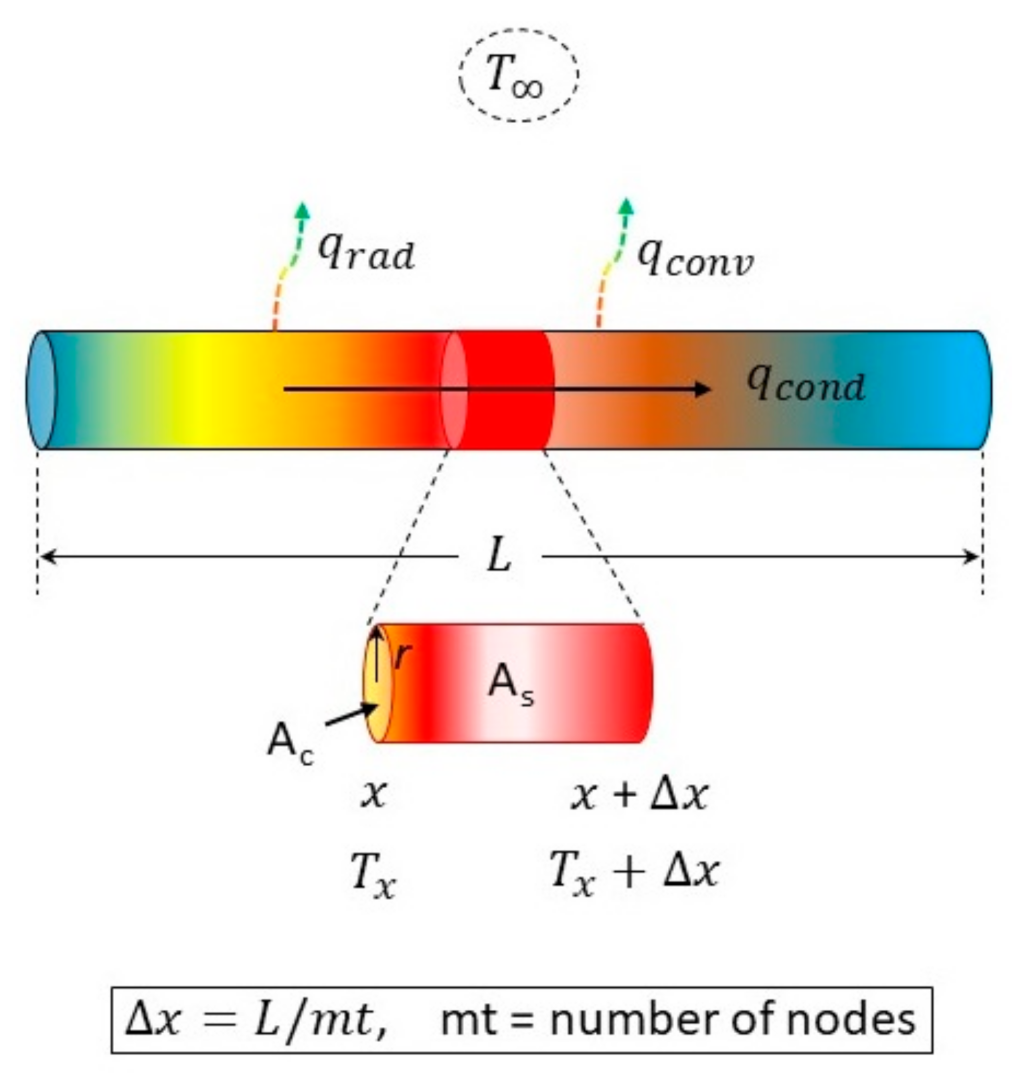
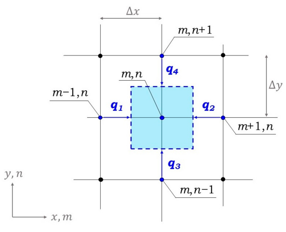
2.2. Numerical Approach

To achieve the aims of this project, it was necessary to establish standards and principles for 3D printing’s main mechanisms. That required an understanding of the principal physical and chemical mechanisms involved in the process: the thermal, mechanical and rheological mechanisms (Figure 3).
As stated previously, the focus of this work is on the thermal mechanisms since knowledge of the temperature distribution along the extrusion may provide valuable information relating to the structural integrity through the determination of thermal stresses, also referred to as stress points. The bonding between filaments and between layers is induced by the thermal energy of the molten material, and as solidification occurs (if the rate of solidification is very fast), the appearance of thermal gradients might create mechanical stresses that result in distortion and detachment of individual filaments, if these are not effectively controlled.
Concerning the thermal mechanisms, these are represented by a relatively simple idea: “The amount of energy stored in a control volume (or medium) must equal the amount of energy that enters, minus the amount of energy that leaves, plus the energy generated within the medium” (Equation (1)) [43].
E s t ˙ = E i n ˙ E o u t ˙ + E g ˙
where E s t ˙ refers to the rate of change of the stored thermal energy, E g ˙ refers to the rate of generated thermal energy, E i n ˙ refers to the rate of thermal energy that enters the medium and E o u t ˙ refers to the rate of thermal energy leaving the medium.
By assuming an incompressible medium (density (ρ) = constant), the material is considered uniform and isotropic, and the specific heat CP is considered temperature independent. A simplified diffusion Equation (2) can hence be inferred [10,43]:
ρ C P T t = λ 2 T +
where λ is the medium thermal conductivity and the term incorporates the generated heat, the heat to the medium and the heat losses to the surroundings.
Equation (2) can be rewritten, as follows, if divided by the medium thermal conductivity [38]:
1 α T t = 2 T +
where the resulting constant α is the thermal diffusivity of the material that is equal to λ ρ C P . This parameter measures the ability of a material to conduct thermal energy relative to its respective ability to store thermal energy.
From the heat diffusion equation, one can determine the temperature transient during the filament manufacturing (Figure 4), which is mainly driven by the heat transfer through conduction ( q c o n d = λ A T x T x + Δ x Δ L ) in the medium (along the x axis direction) and by the heat losses from the filament surface to the surroundings. The latter is referred to as convection ( q c o n v = h A T s T ) and radiation ( q r a d = ε σ A T S 4 T 4 ) losses [43], where T S and T are the surface and the surrounding temperatures, respectively, ε is the filament emissivity and σ is the Stefan–Bolzmann constant (5.67 × 10⁻⁸ (J/s·m2·K4)].
The heat losses are dependent on the surface medium properties. When the surface temperature is lower than that of the surrounding temperature (which is usually not the case), heat is transferred to the medium. Accordingly, heat transfer is defined as thermal energy in transit due to a spatial temperature difference.
Assuming unidirectional heat conduction along the x-axis, the heat flux q c o n d ' ' is normal to the medium cross-sectional area Ac of constant temperature, referred to as the isothermal surface (Figure 4). Isothermal surfaces are planes that are normal to the direction of the heat propagation [43,44].
The heat transfer rate (W = J/s) through a material with length L is driven by the thermal conductivity, the surface area (perpendicular to the direction of the heat wave propagation) and the temperature gradient (the difference in temperature between two points distant by L). The convective heat transfer is proportional to the convective coefficient (h or hconv), the surface area and the temperature difference between the medium surface temperature and the surrounding temperature. An equivalent formulation can be formulated for radiation losses.
Recognizing that the heat flux is a directional quantity, a more general conduction rate equation, known as Fourier’s law, is as follows [43]:
q = q A = λ T = λ i T x + j T x + k T x
where q is the heat flux (W/m2) or heat transfer rate (W) per unit area (m2), perpendicular to the direction of transfer; q is the heat rate (W = J/s); i, j and k are the unit vectors along x, y and z, respectively; and T is a scalar temperature field. The minus sign is a consequence of heat being transferred toward the direction of decreasing temperature.
An alternative form of Fourier’s law is represented as follows [43]:
q = q l '' = λ T n l
where q l '' is the heat flux (W/m2) in the directional unit normal vector l.
Since the governing equations do not allow for obtaining simple analytical solutions, numerical algorithms were employed to determine the heat transfer by conduction in the medium, and the heat loss transfer from the medium to the surrounding atmosphere. The required understanding of the respective systems increases with the complexity of the piece to print. Thus, the assistance by numerical simulations is expected to minimize flaws that are naturally related to additive manufacturing processes. These flaws can be thermally related, such as from stress and strain, and attributed to high gradient levels between extruded filaments.
By considering a 2D case study, the numerical discretization of the problem was achieved by the transformation of our medium (or domain) into several smaller domains, thus creating a mesh through each lane (oriented in either the x- or y-axis) where the heat conduction evolved (Figure 5) [43].
Considering this example, the temperature at the (m, n) node is the result of the heat contributions from several adjacent neighboring nodes, with the heat flux being normal to isotherm surfaces.
Since a 2D problem is under analysis, the isotherm surfaces (blue dashed lines, normal to the heat flux—Figure 5) are given by Δ x × Δ y , where Δ z = 1 . When performing such an exercise, the heat flux (transferred by conduction) from the left node (m − 1, n) to the interior node (m, n) is given by Equation (6). The same is applicable for the remaining nodes (Equations (7)–(9)) [43].
q m 1 , n m , n = λ Δ y · 1 T m 1 , n T m , n Δ x
q m + 1 , n m , n = λ Δ y · 1 T m + 1 , n T m , n Δ x
q m , n 1 m , n = λ Δ x · 1 T m , n 1 T m , n Δ y
q m , n + 1 m , n = λ Δ x · 1 T m , n + 1 T m , n Δ y
Assuming Δ x = Δ y , the summation of each contribution gives [43]
1 4 T m 1 , n + T m + 1 , n + T m , n 1 + T m , n + 1 4 T m , n
For the discretization of the numerical problem, the implementation of the present finite-difference equations follows the energy balance methodology [43]. This approach allows for the analysis of many different phenomena, such as those involving multiple materials, embedded heat sources and exposed surfaces that do not align with an axis of the coordinate system. In the energy balance method, the finite-difference equation for a node is obtained by applying the conservation of energy law to a control volume around the nodal region. This formulation assumes that the entire heat flow is within the control volume represented by the (m, n) node.
Remembering the heat diffusion equation, ρ C P δ V T t = δ V λ 2 T + , the summation equals the first term at the right of the equal sign δ V λ 2 T .
Assuming that there are no heat losses and solving for the nodal temperature (m, n) at time (t + 1), and applying the finite-difference forward method to the first derivative of temperature with respect to time, T t = T m , n t + 1 T m , n t Δ t , the temperature time-dependent equation for node m, n will be given by the following Equation [43]:
T m , n t + 1 = F o T m 1 , n t + T m + 1 , n t + T m , n 1 t + T m , n + 1 t + 1 4 F o T m , n t ,
where F o = α Δ t Δ x 2 is referred to as Fourier’s number.
This approach can easily be extended to one- (1D) or three-dimensional (3D) systems.
For 1D, the explicit form of the finite-difference equation for an interior node m reduces to
T m t + 1 = F o T m 1 t + T m + 1 t + 1 2 F o T m t
Considering a uniform temperature distribution across the filament cross-sectional area Ac, or considering a case where radial heat transfer along the filament is neglected, and assuming that heat losses occur from a cylindrical extruded filament with surface area A S = 2 r π Δ x (Figure 4), the numerical temperature diffusion equation, representative of the extrusion process, can be written as [43,44]:
T m t + 1 = F o T m 1 t + T m + 1 t + 1 2 F o T m t h T m t T σ T m t 4 T 4
where h = 2 h ρ C P Δ t r and σ = 2 σ ε ρ C P Δ t r .
Equation (13) is the representation of the finite-difference discretization of Equation (2), when considering a 1D case [43]. The temperature simulation along the filament axis, when considering temperature changes due to heat losses, which immediately impact the temperature along the filament element, is by this means parameterized.
A similar exercise can be applied to a more realistic case, such as an elliptical filament, as with that of the present case study.
Given the differences between the mass of the bed and that of the filament, heat transfer with the bed can be considered in the form of convection. The boundary conditions at the filament edges were considered to be equal to the bed temperature: T (x < 0 and x > 50 mm) = Tbed.

3. Results

This work followed three research paths, with the focus on the development of numerical algorithms, models and simulations for the extrusion of a polymeric material such as ABS. The first numerical model was developed using MATLAB (https://www.mathworks.com/products/matlab.html/, accessed on 20 September 2023), and followed by other simulations using COMSOL Multiphysics software (http://www.comsol.com/, accessed on 20 September 2023). Finally, to validate the simulation of the temperature evolution or profile along an extruded filament, experimental real-time measurements were taken using the FLIR SC5650 infrared camera [41].

3.1. Numerical Models

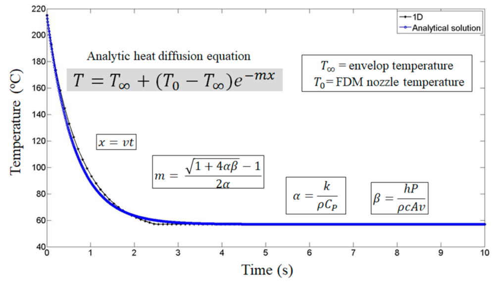
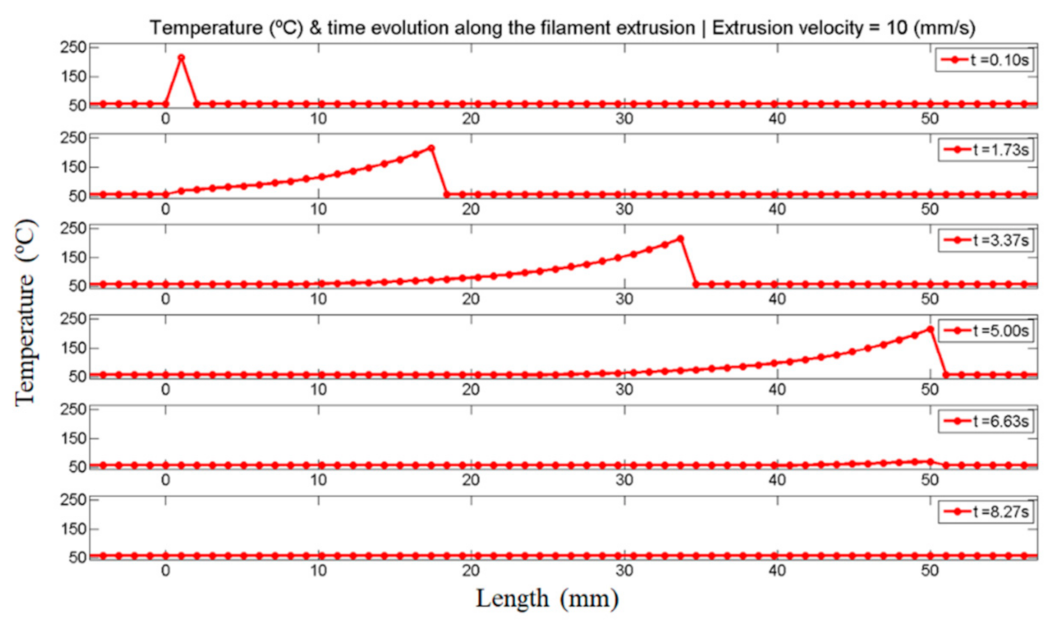
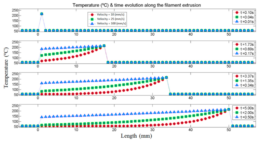
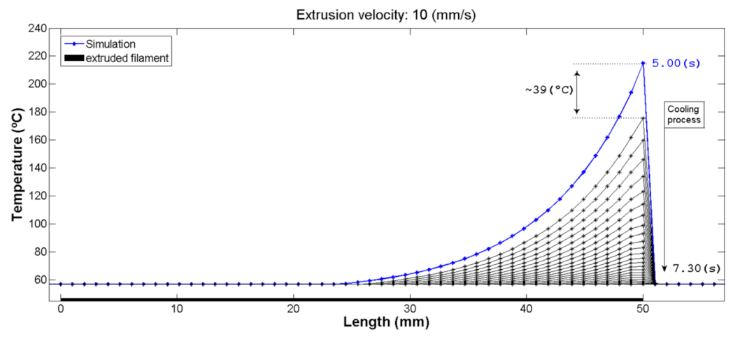
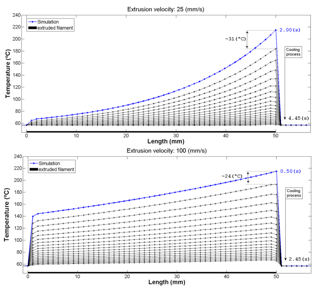
3.1.1. MATLAB Simulation

In the simulation of the temperature evolution during the extrusion process (Equation (13)), the temperature–time cooling process was compared to the 1D analytic heat diffusion equation [10,30]. Figure 6 depicts both analytic and numeric solutions of the cooling curve of the ABS filament with 50 mm length. It takes around 2–2.5 s (as in [35] and [45]) for the filament to cool down to the bed temperature. Figure 7 presents a snapshot of the temperature evolution during the extrusion of the ABS filament with a velocity of 10 mm/s, reaching the 50 mm mark after 5 s, and reaching the bed temperature at ~7 s.
Figure 8 presents a snapshot of the extrusion of the ABS filament with a 50 mm length, at extrusion velocities of 10, 25 and 100 mm/s. Only snapshots, until the 50 mm length mark is reached, are presented.
Figure 9 shows the cooling-time curves for the extrusion velocities of 10, 25 and 100 mm/s. It is clearly visible the different temperature profiles along the filament length, which depend on the extrusion velocity. An exponential profile is observed for lower velocities, and an almost linear profile is attained for high velocities. Figure 9 shows that the filament almost cooled to the bed temperature after 2.5 s.

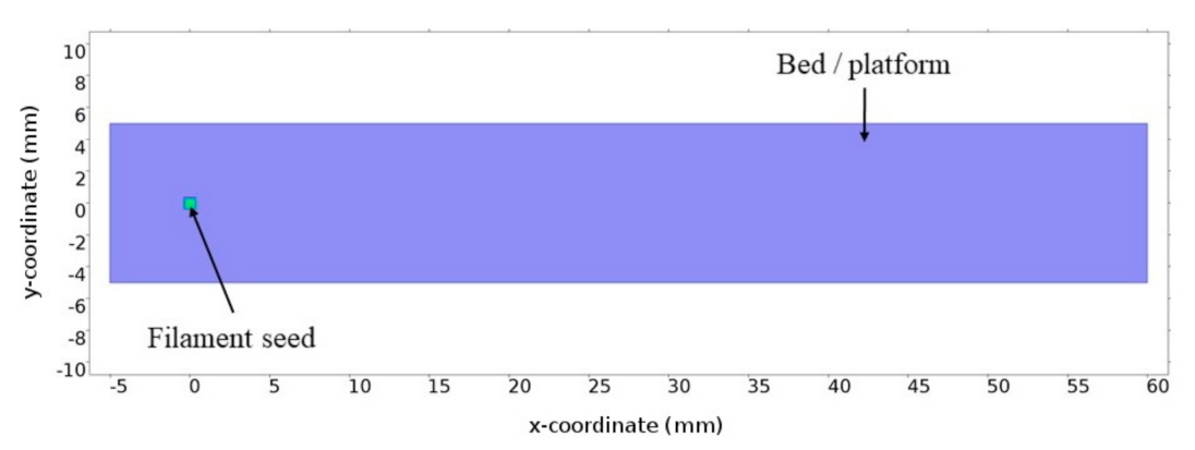
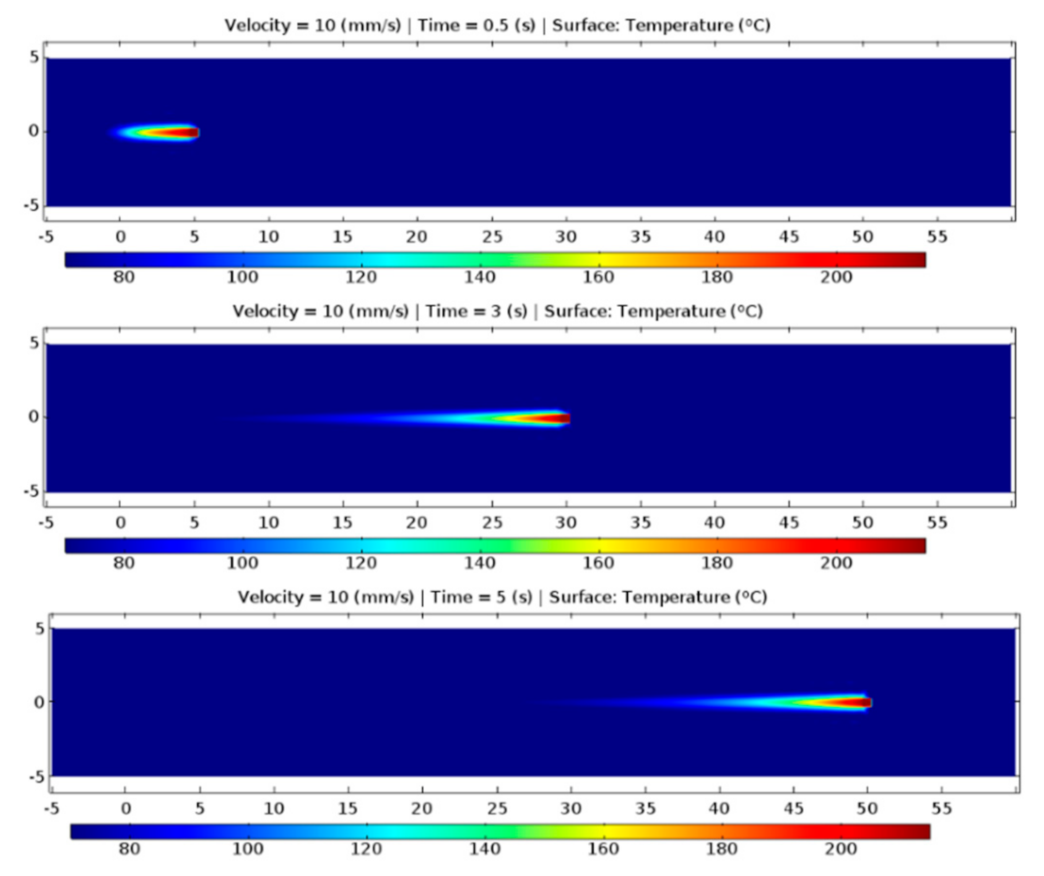
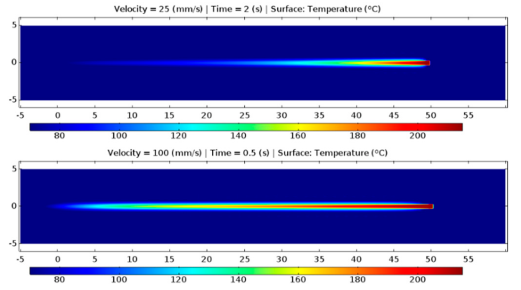
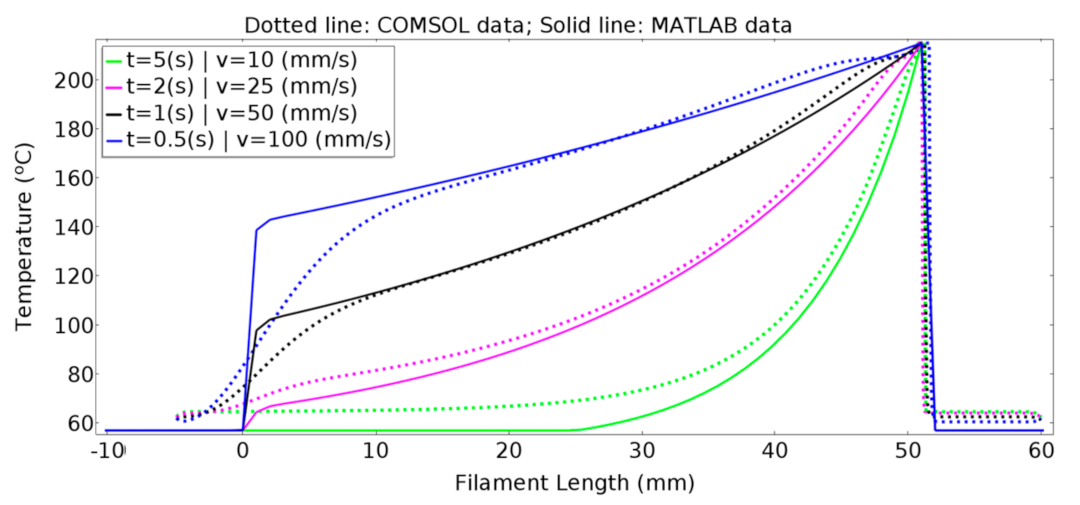
3.1.2. COMSOL Multiphysics Simulation

COMSOL® provides a fully and coupled multi-physics platform, describing specific and highly realistic physics phenomena, producing accurate results. Figure 10 depicts the 2D extrusion bed and the filament seed implemented in COMSOL. This platform was used to relate and validate the numerical algorithm developed in MATLAB.
Heat transfer by conduction between the filament and the bed (out-of-plane, Downside heat flux) and by convection and radiation to the environment (out-of-plane, Upside heat flux) are considered. The filament height, out-of-plane, is equal to 0.2 mm (Table 1). Continuity boundary conditions n d s t · q d s t = n s r c · q s r c and T d s t = T s r c are considered for internal/interface boundaries. n is the (dimensionless) boundary normal vector, q is the boundary conductive heat flux vector and the indexes dst and src refer to the destination and source domains, respectively.
In Figure 11 and Figure 12, surface temperature simulation of the filament extrusion for 10, 25 and 100 mm/s is presented. In Figure 11, the temperature history for three frames corresponding to the positions 5 mm, 30 mm and 50 mm is shown.
Figure 12 depicts the surface temperature for the extrusion velocities of 25 and 100 mm/s after the 50 mm mark length is reached. The surface temperature of the bottom image of Figure 11 (Velocity = 10 mm/s|Time = 5 s) compares with Figure 12 and with the temperature profiles observed in Figure 8 (computed with MATLAB).

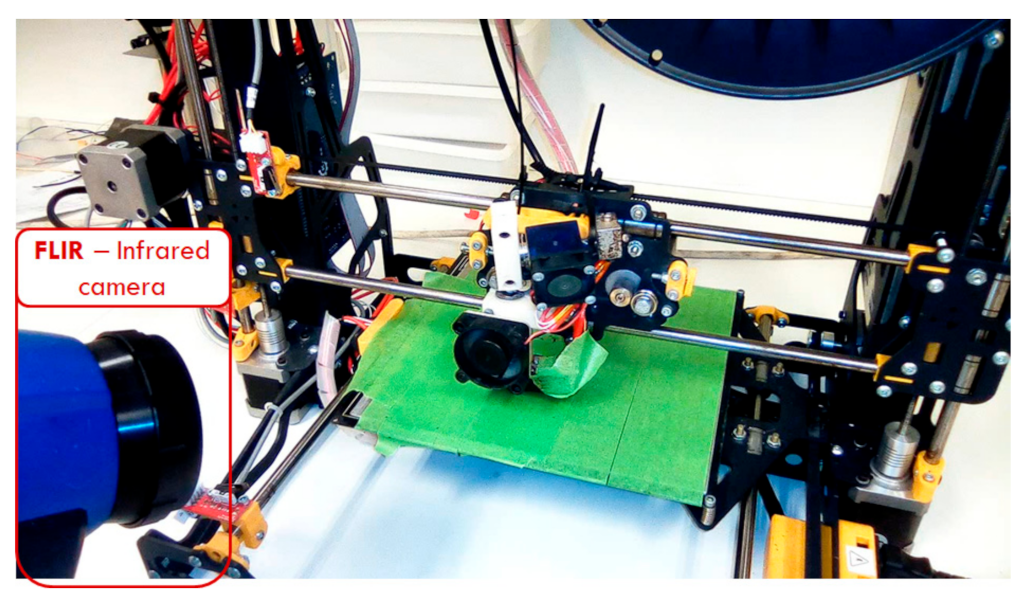
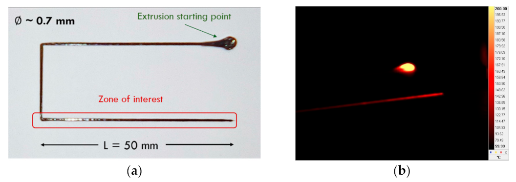
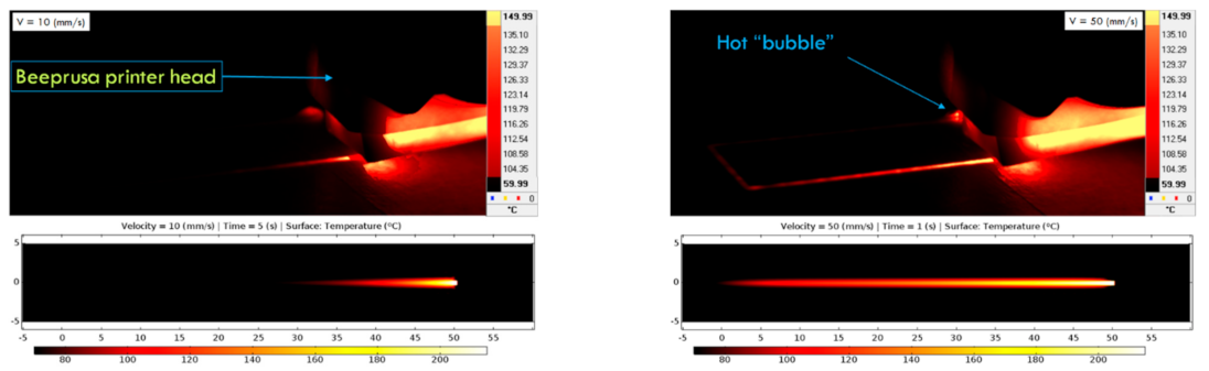
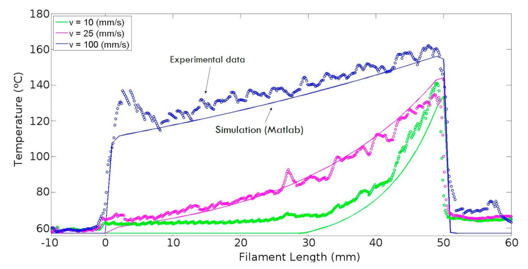
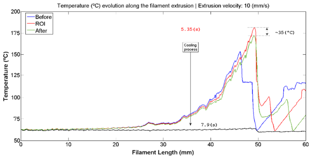
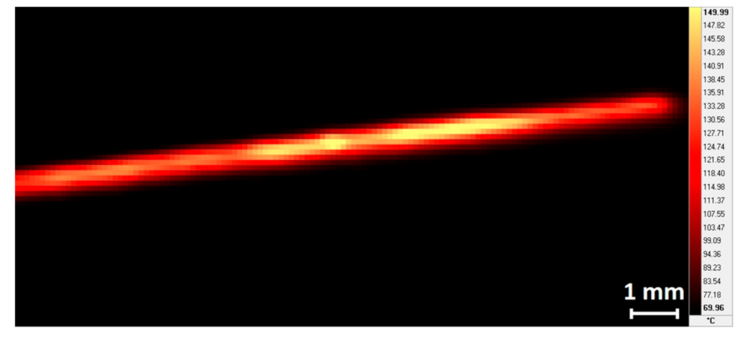
3.2. Experimental Infrared Analysis

Infrared thermal analysis, Figure 13, depicts the measured surface temperature using the FLIR CS5650 infrared camera. Two extrusion case studies are presented, with deposition velocities of 10 and 50 mm/s. The “infrared picture” was captured when the printing nozzle reached the 50 mm filament length. Along with the experimental data/picture, the simulated surface temperature when employing COMSOL is also presented for direct (visual) comparison. An analogous (visual) surface temperature can be observed when comparing those two sets (experiment vs. COMSOL).
After the printing of the U-shaped filament (Figure 2), at the extrusion velocity of 50 mm/s, the “bubble” of the hot material is still visible, which was deposited at the beginning of the filament extrusion. Darker (colder) and brighter (hotter) zones can also be perceived along the filament length. These are attributed to dimensional differences in the filament thickness and height during the extrusion process.

3.3. Overall Remarks

The obtained results (Figure 14) show a fair match between data from simulations of the extrusion phenomenon of a linear 1D ABS filament when using numerical modeling developed throughout the project (using MATLAB software) and when using 2D models in the COMSOL Multiphysics software. Figure 14 shows the temperature variation along a 50 mm long filament for various extrusion velocities.
The experimentally obtained results (FLIR CS5650) for the extrusion of a 0.7 mm thick ABS filament at different speeds, of 10, 25 and 100 mm/s, show good agreement with the numerical results reported in Figure 15. This figure depicts the filament temperature, at the cooling stage, more precisely, taken 0.35 s after the extrusion was finished. This approach was followed after the filament reached the 50 mm length, and it was in line with the infrared camera visibility. The 0.35 s time span was considered so that the extrusion nozzle moves away from the visualization line of the camera, and thus to reduce interferences from the hot extrusion nozzle. This was achieved by sending the nozzle to a position far away from the filament after it reached the 50 mm mark (more precisely for the bed corner that was furthest from the extruded filament), with the nozzle being moved at the maximum velocity of 100 mm/s. The time of 0.35 s was sufficient to remove any external interferences from external hot sources, with direct and indirect interferences from reflection from the bed and the filament surface. These, if captured by the infrared camera, would lead to an incorrect temperature measurement/reading [40]. The interferences/reflections are visible in the experimental (FLIR) videos of the extrusion processes available in the Supplementary Material. Several videos of the simulations are also presented.
Figure 16 depicts what can be considered the error in the evaluation of experimental data, when considering the temperature of the succeeding (“after”) or the previous (“before”) frame with respect to the frame of interest. A difference in the order of a few tens of °C is evident if considering the incorrect frame; each frame is a time span of 0.04 s. The presented data is compared with the equivalent numerical data presented in Figure 9.

4. Discussion

The temperature history plays an important role in the AM; not only does it impact our understanding of the process but it also provides information for optimization and failure prevention.
The infrared thermal analysis yielded information on the temperature evolution during printing, revealing possible thermal gradients or critical cold/hot spots on the parts. In addition to this, information related to the head (“bubble”) and tail effects [43] could also be obtained. Furthermore, experimental data demonstrated that very slight changes in the cross-section of the filament may result in a temperature difference of several degrees. Particular cases are the corners or other locations where the extrusion direction changes. Small dimensional changes in the linear portion of the filament agreed with the observed (experimental—FLIR) temperature changes along respective profile (Figure 13, Figure 15 and Figure 17). As can be clearly observed in Figure 17, during the last millimeters of the extruded filament, a lower temperature was observed due to the tail effect [46].
Valuable information is provided by experimental measurements; however, only the temperature at the surface of the parts can be measured. Not only that, but several other tests are required in order to search for the best visualization angle between the infrared camera and the part(s) being extruded of the printing process, so that errors can be minimized during the temperature measurement. These errors can appear due to direct emission of the infrared camera and reflections of the infrared radiation from external heat sources into the part(s) and the bed, such as those from the hot printing nozzle. These reflections interfere negatively with the temperature measurements [40]. Besides the preparation of the experimental assembly, respective post-processing and analysis is also a relatively onerous process. In contrast, numerical modeling will provide the essential information that allows for the optimization of the experimental setup before entering the laboratory or even the production line.
The numerical 1D model matches the analytical solution in Refs. [10,30], showing that the ABS filament, with similar dimensions and properties as those mentioned in Table 1, cools down to bed temperatures within 2–2.5 s, as was experimentally observed.
In comparison with the 2D model (COMSOL), the numerical 1D (MATLAB) code presents some expected flaws since imprecise dimensional thermal phenomena is simulated when performing such simplifications. All information is condensed into each node. Nevertheless, the 1D numerical model is presented as a valuable tool for the present thermal analysis. The numerical and simplistic model clearly shows the linear/exponential temperature profile dependency on the extrusion velocity, with lower velocities presenting an exponential profile, while for high extrusion velocity, a more linear profile is observed.
The work developed for the 1D numerical model (MATLAB) requires optimization and extrapolation for several other environments and materials. Nevertheless, and considering some experimental aspects related to the fact that the printing process could not be observed in real-time (only perceiving the whole filament a few seconds after deposition due to the nozzle being in the visualization line of the infrared camera), both numerical MATLAB and COMSOL results, and the experimental data, present reliable and comparable information. Moreover, the experimental tests validate the 1D numerical model developed by using the MATLAB software.
The present work was aimed at developing numerical tools that further our understanding of the thermal phenomena intrinsic to the additive manufacturing of polymeric materials, and future optimization. The emphasis was on the study of the temperature evolution during fabrication and its validation. The chosen material was a thermoplastic polymer, more precisely ABS. The process of visualizing the extrusion process at the thermal level was carried out by using an infrared camera, which allowed for comparison of the numerical simulations with the real-time measurements.
It should be noted that the convective heat transfer, more precisely the convective coefficient (hconv), is unknown. This is a material-dependent, object-surface-dimensional and shape-dependent property [38,43]. Moreover, the hconv value that best compares the numerical results with the experimental data is relatively high; nevertheless, it should be taken into account the inclusion of the heat exchangers of the Beeprusa printing equipment. Values for the forced air were found to be within the range of 10 (W/m2·K) and 500 (W/m2·K) [47]. It is noteworthy that the effect of the hconv has a higher impact than the radiation heat losses on the temperature cooling rate [30].
Regardless of some flaws and simplistic approximations of the described model, and considering the COMSOL model, the overall results stand by themselves and are consistent with experimental data and with results found in the literature [10,35,39,45].
As mentioned in Ref. [10], the present approach can be implemented for simple cases; however, 3D-printed parts with higher complexity require more realistic and complex models that may account for the temperature-dependent thermal properties of the materials, such as what is referenced in [33]. Multiphysics simulations, covering other mechanisms responsible for the solidification processes during additive manufacturing of complex objects, such as the conservation of mass (where, in the present case, ρ = constant) and momentum, and the rheologic behavior during printing, are implicit and will be considered for future developments, after the 2D implementation of these features to the present code. Currently, only the conservation of energy for an incompressible flow is considered. FDM process optimization, regardless of the used machine and of the manufactured product, is the ultimate objective.

5. Conclusions

  • Through the use of infrared thermal equipment, thermal gradients and critical spots in the extruded piece or part can be experimentally perceived; however, only those present at the surface are observed.
  • For a better perception of the whole process, and to realize the interior of the parts, and for respective processing optimization, numerical tools are fundamental.
  • The present model is highly simplified,; nevertheless, with the establishment of optimized simulation mechanisms of the printing process (mimicking what experimentally is observed), it is possible to challenge the current printers and determine to what extent these are suitable to print complex objects and optimize those in almost real-time, and according to the limitations of each specific printer, before going to the printing line.
  • By measuring the discrepancy between the output of a concrete printer and the expected theoretical/simulation output, one has an expectancy of the performance for a printer. This will allow for the development of printing strategies, for that same printer, that will best approximate the expected outcome.
  • The acknowledgement and prediction of the temperature and thermal behavior during the printing of an object can help in the search for the best heat source velocity, feed rate, filament or nozzle diameter, composition of the material blend and other parameters, by comparing with those created using the tool path (G-code), thus reducing the thermal gradients and bonding diffusivity of the extruded material, in order to create the object/part with best mechanical properties. These will result in part with better geometry and less residue during fabrication.
  • It is thus expected that improvement of the features of the product will ultimately preserve natural resources and promote environmental and economic benefits by obtaining cleaner and environmentally friendly solutions for material processing.
Our project aimed further the existing knowledge and promote future development and implementation of machine learning algorithms, which will take into account the most important/impactful mechanisms of 3D printing, and will aid in the search for the best, most efficient and robust filling strategies that will produce the product with optimal properties for the intended applications. The primitive-deposited road is discretized according to the optimal predicted path that potentiates a more homogeneous temperature in all the parts during fabrication, independently of the design (3D CAD object) and the used machine. Such a strategy will reduce the number of defects and flaws during printing that may occur due to thermal gradients and stress point formation of thermal origin.

Supplementary Materials

The following supporting information can be downloaded at https://www.mdpi.com/article/10.3390/jmmp7060189/s1.

Author Contributions

Conceptualization, T.S., M.B. and N.F.; methodology, T.S.; software, T.S., M.B., J.A., V.A. and N.F.; validation, T.S., M.B. and N.F.; formal analysis, T.S., M.B., N.A., P.P.-F. and N.F.; investigation, T.S.; resources, T.S., M.B., J.A., V.A., N.F., N.A. and P.P.-F.; data curation, T.S.; writing—original draft preparation, T.S.; writing—review and editing, T.S., M.B., J.A., V.A., N.F., N.A. and P.P.-F.; visualization, T.S.; supervision, T.S., J.A., N.A., P.P.-F. and N.F.; project administration, T.S., J.A., V.A., N.F., N.A. and P.P.-F.; funding acquisition, J.A., V.A., N.F., N.A. and P.P.-F. All authors have read and agreed to the published version of the manuscript.

Funding

This work was financially supported by the Fundação para a Ciência e a Tecnologia FCT/MCTES (PIDDAC) through the following projects: UIDB/04044/2020 and UIDP/04044/2020; Associate Laboratory ARISE LA/P/0112/2020; PAMI—ROTEIRO/0328/2013 (No 022158); FCT projects Stimuli2BioScaffold (PTDC/EMESIS/32554/2017), OptiBioScaffold (PTDC/EMESIS/4446/2020) MATIS (CENTRO-01-0145-FEDER-000014-3362); and projects of the CICECO-Aveiro Institute of Materials (UIDB/50011/2020, UIDP/50011/2020 and LA/P/0006/2020), financed by national funds through the FCT/MCTES (PIDDAC).

Institutional Review Board Statement

Not applicable.

Informed Consent Statement

Not applicable.

Data Availability Statement

Not applicable.

Acknowledgments

The authors express their sincere thanks to João Pinheiro and Luiz Fonseca, from CDRSP—Centre for Rapid and Sustainable Product Development, Polytechnic Institute of Leiria, 2430-028 Marinha Grande, Portugal, for their help, contributions and technical support in operating the Beeprusa printer machine. Acknowledgment is also due to E. Lora da Silva for proofreading the article.

Conflicts of Interest

The authors declare no conflict of interest. The funders had no role in the design of the study; in the collection, analyses or interpretation of data; in the writing of the manuscript; or in the decision to publish the results.

References

  1. Hull, C. On Stereolithography. Virtual Phys. Prototyp. 2012, 7, 177. [Google Scholar] [CrossRef]
  2. Raja, S.; Agrawal, A.P.; Patil, P.; Thimothy, P.; Capangpangan, R.Y.; Singhal, P.; Wotango, M.T. Optimization of 3D Printing Process Parameters of Polylactic Acid Filament Based on the Mechanical Test. Int. J. Chem. Eng. 2022, 2022, 5830869. [Google Scholar] [CrossRef]
  3. Jandyal, A.; Chaturvedi, I.; Wazir, I.; Raina, A.; Ul Haq, M.I. 3D Printing—A Review of Processes, Materials and Applications in Industry 4.0. Sustain. Oper. Comput. 2022, 3, 33–42. [Google Scholar] [CrossRef]
  4. Subramani, R.; Kaliappan, S.; Sekar, S.; Patil, P.P.; Usha, R.; Manasa, N.; Esakkiraj, E.S. Polymer Filament Process Parameter Optimization with Mechanical Test and Morphology Analysis. Adv. Mater. Sci. Eng. 2022, 2022, 8259804. [Google Scholar] [CrossRef]
  5. Godec, D.; Gonzalez-Gutierrez, J.; Nordin, A.; Pei, E.; Ureña Alcázar, J. (Eds.) A Guide to Additive Manufacturing. In Springer Tracts in Additive Manufacturing, 1st ed.; Springer International Publishing: Cham, Switzerland, 2022; ISBN 978-3-031-05862-2. [Google Scholar]
  6. Jaisingh Sheoran, A.; Kumar, H. Fused Deposition Modeling Process Parameters Optimization and Effect on Mechanical Properties and Part Quality: Review and Reflection on Present Research. Mater. Today Proc. 2020, 21, 1659–1672. [Google Scholar] [CrossRef]
  7. What Are the Advantages and Disadvantages of 3D Printing?—TWI. Available online: https://www.twi-global.com/technical-knowledge/faqs/what-is-3d-printing/pros-and-cons#Consof3DPrinting (accessed on 9 March 2021).
  8. Turner, B.N.; Strong, R.; Gold, S.A. A Review of Melt Extrusion Additive Manufacturing Processes: I. Process Design and Modeling. Rapid Prototyp. J. 2014, 20, 192–204. [Google Scholar] [CrossRef]
  9. Li, Q.; Kucukkoc, I.; Zhang, D.Z. Production Planning in Additive Manufacturing and 3D Printing. Comput. Oper. Res. 2017, 83, 1339–1351. [Google Scholar] [CrossRef]
  10. Zhang, Y.; Shapiro, V. Linear-Time Thermal Simulation of as-Manufactured Fused Deposition Modeling Components. J. Manuf. Sci. Eng. Trans. ASME 2018, 140, 071002. [Google Scholar] [CrossRef]
  11. Jornadas CICECO 2018—Universidade de Aveiro News. Available online: https://www.ua.pt/pt/noticias/0/54604 (accessed on 9 March 2021).
  12. 3D Printed Violin: 6 Most Amazing Projects|All3DP. Available online: https://all3dp.com/2/3d-printed-violin-6-most-amazing-projects/ (accessed on 9 March 2021).
  13. Choi, J.H.; Kang, E.T.; Lee, J.W.; Kim, U.S.; Cho, W.S. Materials and Process Development for Manufacturing Porcelain Figures Using a Binder Jetting 3D Printer. J. Ceram. Process. Res. 2018, 19, 43–49. [Google Scholar]
  14. Chen, Z.; Li, Z.; Li, J.; Liu, C.; Lao, C.; Fu, Y.; Liu, C.; Li, Y.; Wang, P.; He, Y. 3D Printing of Ceramics: A Review. J. Eur. Ceram. Soc. 2019, 39, 661–687. [Google Scholar] [CrossRef]
  15. Tosto, C.; Bragaglia, M.; Nanni, F.; Recca, G. Fused Filament Fabrication of Alumina/Polymer Filaments for Obtaining Ceramic Parts after Debinding and Sintering Processes. Materials 2022, 15, 7399. [Google Scholar] [CrossRef] [PubMed]
  16. Revelo, C.F.; Colorado, H.A. 3D Printing of Kaolinite Clay Ceramics Using the Direct Ink Writing (DIW) Technique. Ceram. Int. 2018, 44, 5673–5682. [Google Scholar] [CrossRef]
  17. Santos, T.; Ramani, M.; Devesa, S.; Batista, C.; Franco, M.; Duarte, I.; Costa, L.; Ferreira, N.; Alves, N.; Pascoal-faria, P. A 3D-Printed Ceramics Innovative Firing Technique: A Numerical and Experimental Study. Materials 2022, 16, 6236. [Google Scholar] [CrossRef] [PubMed]
  18. Camarero-Espinosa, S.; Moroni, L. Janus 3D Printed Dynamic Scaffolds for Nanovibration-Driven Bone Regeneration. Nat. Commun. 2021, 12, 1031. [Google Scholar] [CrossRef] [PubMed]
  19. Pattanashetti, N.A.; Viana, T.; Alves, N.; Mitchell, G.R.; Kariduraganavar, M.Y. Development of Novel 3D Scaffolds Using BioExtruder by Varying the Content of Hydroxyapatite and Silica in PCL Matrix for Bone Tissue Engineering. J. Polym. Res. 2020, 27, 87. [Google Scholar] [CrossRef]
  20. Arif, Z.U.; Khalid, M.Y.; Noroozi, R.; Sadeghianmaryan, A.; Jalalvand, M.; Hossain, M. Recent Advances in 3D-Printed Polylactide and Polycaprolactone-Based Biomaterials for Tissue Engineering Applications. Int. J. Biol. Macromol. 2022, 218, 930–968. [Google Scholar] [CrossRef]
  21. Lee, C.Y.; Liu, C.Y. The Influence of Forced-Air Cooling on a 3D Printed PLA Part Manufactured by Fused Filament Fabrication. Addit. Manuf. 2019, 25, 196–203. [Google Scholar] [CrossRef]
  22. Most Used 3D Printing Technologies 2020|Statista. Available online: https://www.statista.com/statistics/560304/worldwide-survey-3d-printing-top-technologies/ (accessed on 9 March 2021).
  23. Kokkinis, D.; Schaffner, M.; Studart, A.R. Multimaterial Magnetically Assisted 3D Printing of Composite Materials. Nat. Commun. 2015, 6, 8643. [Google Scholar] [CrossRef]
  24. Dey, A.; Roan Eagle, I.N.; Yodo, N. A Review on Filament Materials for Fused Filament Fabrication. J. Manuf. Mater. Process. 2021, 5, 69. [Google Scholar] [CrossRef]
  25. Xia, H.; Lu, J.; Tryggvason, G. Fully Resolved Numerical Simulations of Fused Deposition Modeling. Part II—Solidification, Residual Stresses and Modeling of the Nozzle. Rapid Prototyp. J. 2018, 24, 973–987. [Google Scholar] [CrossRef]
  26. Xia, H.; Lu, J.; Dabiri, S.; Tryggvason, G. Fully Resolved Numerical Simulations of Fused Deposition Modeling. Part I: Fluid Flow. Rapid Prototyp. J. 2018, 24, 463–476. [Google Scholar] [CrossRef]
  27. Alic, A. Physics of 3D Printing; Ljubljana, Slovenia, 2017. Available online: https://www.scribd.com/document/480834295/Amina-Alic-seminar-1b-pdf (accessed on 26 October 2020).
  28. Blanco, I. A Brief Review of the Applications of Selected Thermal Analysis Methods to 3D Printing. Thermo 2022, 2, 74–83. [Google Scholar] [CrossRef]
  29. Zhang, Y.; Chou, Y. Three-Dimensional Finite Element Analysis Simulations of the Fused Deposition Modelling Process. Proc. Inst. Mech. Eng. Part B J. Eng. Manuf. 2006, 220, 1663–1671. [Google Scholar] [CrossRef]
  30. Bellehumeur, C.; Li, L.; Sun, Q.; Gu, P. Modeling of Bond Formation between Polymer Filaments in the Fused Deposition Modeling Process. J. Manuf. Process. 2004, 6, 170–178. [Google Scholar] [CrossRef]
  31. Marques, B.M.; Andrade, C.M.; Neto, D.M.; Oliveira, M.C.; Alves, J.L.; Menezes, L.F. Numerical Analysis of Residual Stresses in Parts Produced by Selective Laser Melting Process. Procedia Manuf. 2020, 47, 1170–1177. [Google Scholar] [CrossRef]
  32. Zhang, Y.; Chou, K. A Parametric Study of Part Distortions in Fused Deposition Modelling Using Three-Dimensional Finite Element Analysis. Proc. Inst. Mech. Eng. Part B J. Eng. Manuf. 2008, 222, 959–967. [Google Scholar] [CrossRef]
  33. Ji, L.; Zhou, T. Finite Element Simulation of Temperature Field in Fused Deposition Modeling. Adv. Mater. Res. 2010, 97-101, 2585–2588. [Google Scholar] [CrossRef]
  34. Yardimci, M.A.; Güçeri, S. Conceptual Framework for the Thermal Process Modelling of Fused Deposition. Rapid Prototyp. J. 1996, 2, 26–31. [Google Scholar] [CrossRef]
  35. Sun, Q.; Rizvi, G.M.; Bellehumeur, C.T.; Gu, P. Effect of Processing Conditions on the Bonding Quality of FDM Polymer Filaments. Rapid Prototyp. J. 2008, 14, 72–80. [Google Scholar] [CrossRef]
  36. Li, L.; Sun, Q.; Bellehumeur, C.; Gu, P. Investigation of Bond Formation in FDM Process. Trans. North Am. Manuf. Res. Inst. SME 2019, 31, 400–407. [Google Scholar]
  37. Pokluda, O.; Bellehumeur, C.T.; Vlachopoulos, J. Modification of Frenkel’s Model for Sintering. AIChE J. 1997, 43, 3253–3256. [Google Scholar] [CrossRef]
  38. Costa, S.F.; Duarte, F.M.; Covas, J.A. Estimation of Filament Temperature and Adhesion Development in Fused Deposition Techniques. J. Mater. Process. Technol. 2017, 245, 167–179. [Google Scholar] [CrossRef]
  39. Costa, S.F.; Duarte, F.M.; Covas, J.A. Thermal Conditions Affecting Heat Transfer in FDM/FFE: A Contribution towards the Numerical Modelling of the Process. Virtual Phys. Prototyp. 2015, 10, 35–46. [Google Scholar] [CrossRef]
  40. FLIR Photometry Form: FLIR DG001U-E. pp. 1-56.
  41. FLIR Advanced Thermal Solutions DCOO2U-L SC5000 User Manual.
  42. Rahman, M.; Schott, N.R.; Sadhu, L.K. Glass Transition of ABS in 3D Printing. In Proceedings of the COMSOL Conference, Boston, MA, USA, 5–7 October 2016; pp. 1–5. [Google Scholar]
  43. Incropera, F.P.; DeWitt, D.P.; Bergman, L.T.; Lavine, A.S. Fundamentals of Heat and Mass Transfer, 6th ed.; John Wiley Sons: Hoboken, NJ, USA, 2007. [Google Scholar]
  44. Chapra, S.C. Applied Numerical Methods with MATLAB for Engineers and Scientists, 3rd ed.; Lange, M., Massar, P.E., Buczek, L., Eds.; Raghothaman Srinivasan: New York, NY, USA, 2012; ISBN 978-0-07-339796-2. [Google Scholar]
  45. McIlroy, C.; Olmsted, P.D. Disentanglement Effects on Welding Behaviour of Polymer Melts during the Fused-Filament-Fabrication Method for Additive Manufacturing. Polymer 2017, 123, 376–391. [Google Scholar] [CrossRef]
  46. Li, W.; Ghazanfari, A.; Leu, M.C.; Landers, R.G. Extrusion-on-Demand Methods for High Solids Loading Ceramic Paste in Freeform Extrusion Fabrication. Virtual Phys. Prototyp. 2017, 12, 193–205. [Google Scholar] [CrossRef]
  47. Kosky, P.; Balmer, R.; Keat, W.; Wise, G. (Eds.) Mechanical Engineering. In Exploring Engineering—An Introduction to Engineering and Design; Academic Press: Waltham, MA, USA, 2013; Chapter 12; pp. 259–281. ISBN 9780124158917. [Google Scholar]
Figure 1. Experimental setup.
Jmmp 07 00189 g001
Figure 2. U-shaped printed filament: (a) photograph, highlighting the linear part/region of interest (ROI) with 50 mm length (L) and an approximate thickness (ϕ) of 0.7 mm; (b) thermograph image showing the hotter bubble, after a few seconds following the end of the extrusion process.
Jmmp 07 00189 g002
Figure 3. Main mechanisms in 3D printing.
Jmmp 07 00189 g003
Figure 4. Representation of the heat balance for a filament element subject to conduction, convection and radiation heat flow.
Jmmp 07 00189 g004
Figure 5. Classical numerical schematization of a 2D heat flux or conduction to an interior domain node.
Jmmp 07 00189 g005
Figure 6. Temperature variation determined by the implemented numerical method (1D: black curve) and compared with the analytical solution (blue curve), as described in [2,3].
Jmmp 07 00189 g006
Figure 7. Temperature snapshots mimicking the extrusion, v = 10 mm/s, of the ABS filament with L = 50 mm.
Jmmp 07 00189 g007
Figure 8. Temperature snapshots mimicking the extrusion of the ABS filament with L = 50 mm for several extrusion velocities (10, 25 and 100 mm/s).
Jmmp 07 00189 g008
Figure 9. Temperature profile along the filament of 50 mm length presenting the cooling–time curves for the extrusion velocities of 10, 25 and 100 mm/s. The line in blue represents the time instant at which the extrusion head reached the 50 mm length.
Jmmp 07 00189 g009aJmmp 07 00189 g009b
Figure 10. Developed model using COMSOL Multiphysics: 2D bed and filament seed.
Jmmp 07 00189 g010
Figure 11. COMSOL temperature surface plot for the extrusion velocity of 10 mm/s and for the time instants 0.5 s, 3 s and 5 s.
Jmmp 07 00189 g011
Figure 12. COMSOL temperature surface plot for the extrusion velocities of 25 and 100 mm/s and after the simulation reached the 50 mm length mark.
Jmmp 07 00189 g012
Figure 13. Experimental (FLIR) and COMSOL simulation of the surface temperature along the 50 mm length filament extruded at 10 and 50 mm/s.
Jmmp 07 00189 g013
Figure 14. Temperature profile simulation for various extrusion speeds. MATLAB profiles are represented in solid lines (–) and COMSOL in dotted lines (…).
Jmmp 07 00189 g014
Figure 15. Experimental temperature profile of the 50 mm ABS extrusion and comparison with numerical (MATLAB) temperature profile.
Jmmp 07 00189 g015
Figure 16. Experimental temperature profile of the extruded (50 mm) ABS filament, showing three consecutive time instants or frames of the cooling process. The “Before” and “After” frames are shown with respect to the frame of interest “ROI”. In the “Before” frame, the extrusion nozzle is still in the visualization line of the infrared camera, which is the reason why the respective temperature profile is not fully observed. It also presents the time instant at which the filament is almost at the bed temperature.
Jmmp 07 00189 g016
Figure 17. Experimental FLIR temperature map of the last millimeters of the filament, extruded at 100 mm/s. Image taken after the extrusion finished and for one test where the filament section suffered some dimensional modification due to the high extrusion velocity and consequently lower adherence to the bed (the section of the last millimeters presents a smaller cross-section as depicted in Figure 2a, showing tail effects [46]).
Jmmp 07 00189 g017
Table 1. Material input parameters [26].
MaterialDensity
ρ
(kg/m3)
Specific Heat
CP
(J/kg·K)
Thermal
Conductivity
λ
(W/m·K)
Length
L
(mm)
Thickness
ϕ
(mm)
Height
h
(mm)
ABS105020800.17750~0.7~0.2
hABS (ABS convective heat transfer coefficient considered in the simulations) = 250 (W/m2·K).
Disclaimer/Publisher’s Note: The statements, opinions and data contained in all publications are solely those of the individual author(s) and contributor(s) and not of MDPI and/or the editor(s). MDPI and/or the editor(s) disclaim responsibility for any injury to people or property resulting from any ideas, methods, instructions or products referred to in the content.

