
A Comparative Study of a Machine Learning Approach and Response Surface Methodology for Optimizing the HPT Processing Parameters of AA6061/SiCp Composites

 , , , , , ,
Abstract
:1. Introduction
2. Methodology
2.1. Materials and Experimental Procedures
2.2. Machine Learning (ML) Approach
- Data preparation: This step includes collecting the data, cleaning, feature engineering, and normalization.
- Data splitting: The data are split into training and testing sets. Optionally, the data can also be split into validation sets to tune hyperparameters.
- Model defining: This step includes choosing a machine learning algorithm and defining the model architecture.
- Model training: The model is trained on the training dataset using the chosen algorithm and hyperparameters.
- Model evaluation: The model is tested on the testing dataset to evaluate its performance. Optionally, the validation set can also be used to tune hyperparameters.
- Cross-validation: k-fold cross-validation is performed to estimate the performance of the model on new, unseen data. This step is repeated with different random splits of the data, and the results are averaged to increase the reliability of the estimate.
- Hyperparameter tuning: The results of cross-validation are used to tune the hyperparameters of the model, such as the learning rate, regularization strength, or number of layers.
- Evaluation of the final model: after training the final model on the entire dataset using the optimized hyperparameters, it is important to test the final model on a holdout dataset to evaluate its performance on new, unseen data.
- Model deployment: The final model is deployed in production, and its performance over time is monitored.
2.2.1. Multivariable Linear Regression
2.2.2. Regression Gaussian Process
2.2.3. Support Vector Machine
2.2.4. Analysis of ML Approach
2.3. Statistical Analysis
3. Results and Discussion
3.1. Relative Density (RD)
3.1.1. Machine Learning Prediction Models of Relative Density
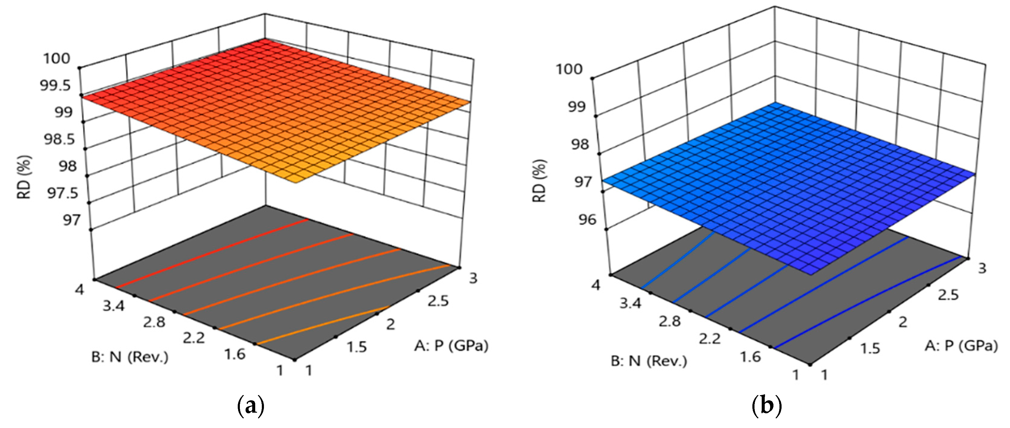
3.1.2. Regression Models and 3D Plots of Relative Density
3.1.3. Optimization of Relative Density
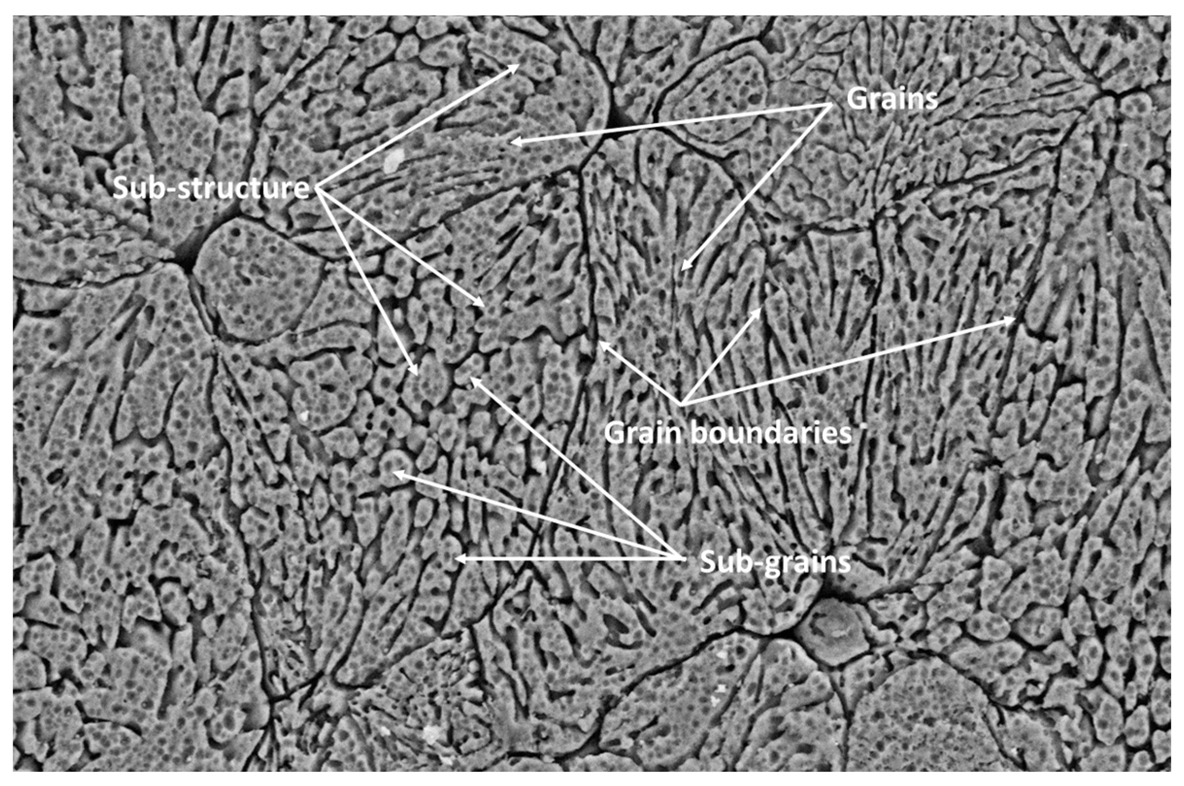
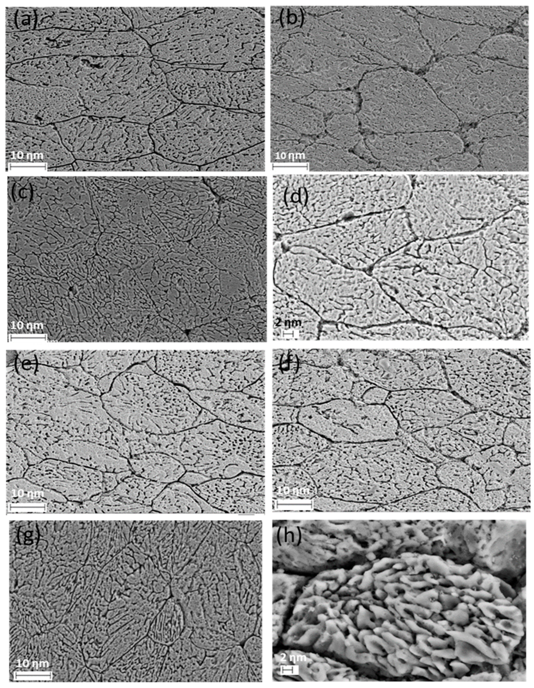
3.2. Microstructural Evolution
3.2.1. Machine Learning Prediction Models of the Microstructural Evolution
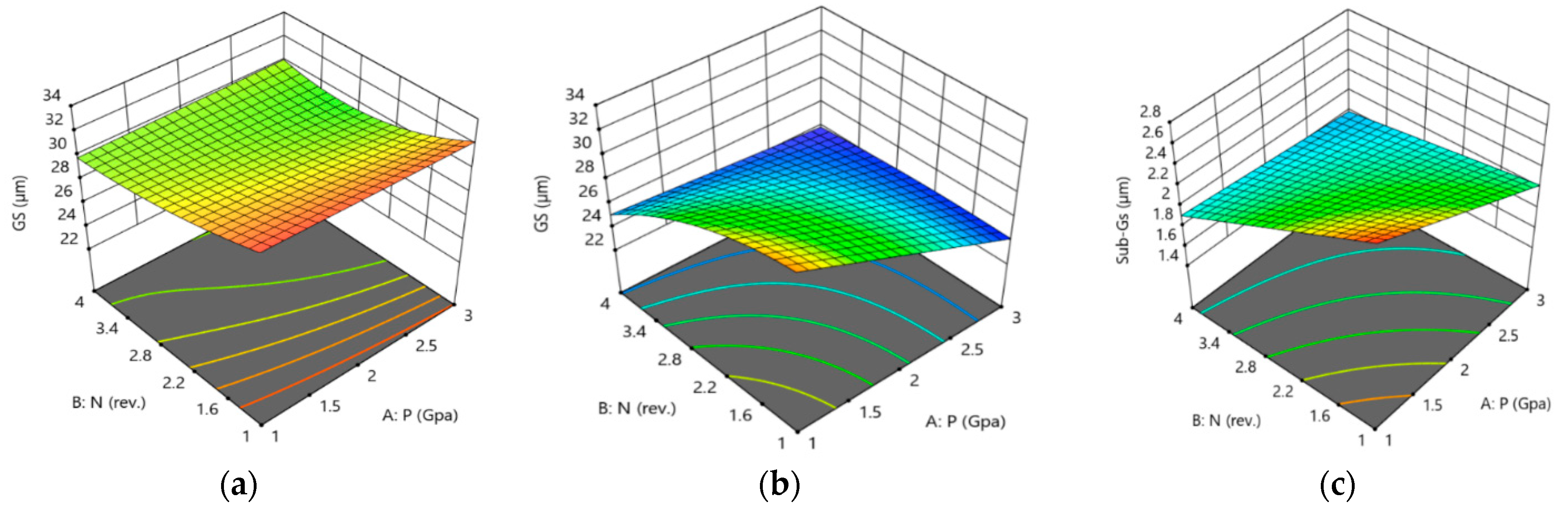
3.2.2. Regression Models and 3D Plots of Microstructure Characteristics
3.2.3. Optimization of Microstructure Characteristics
3.3. Hardness Distribution
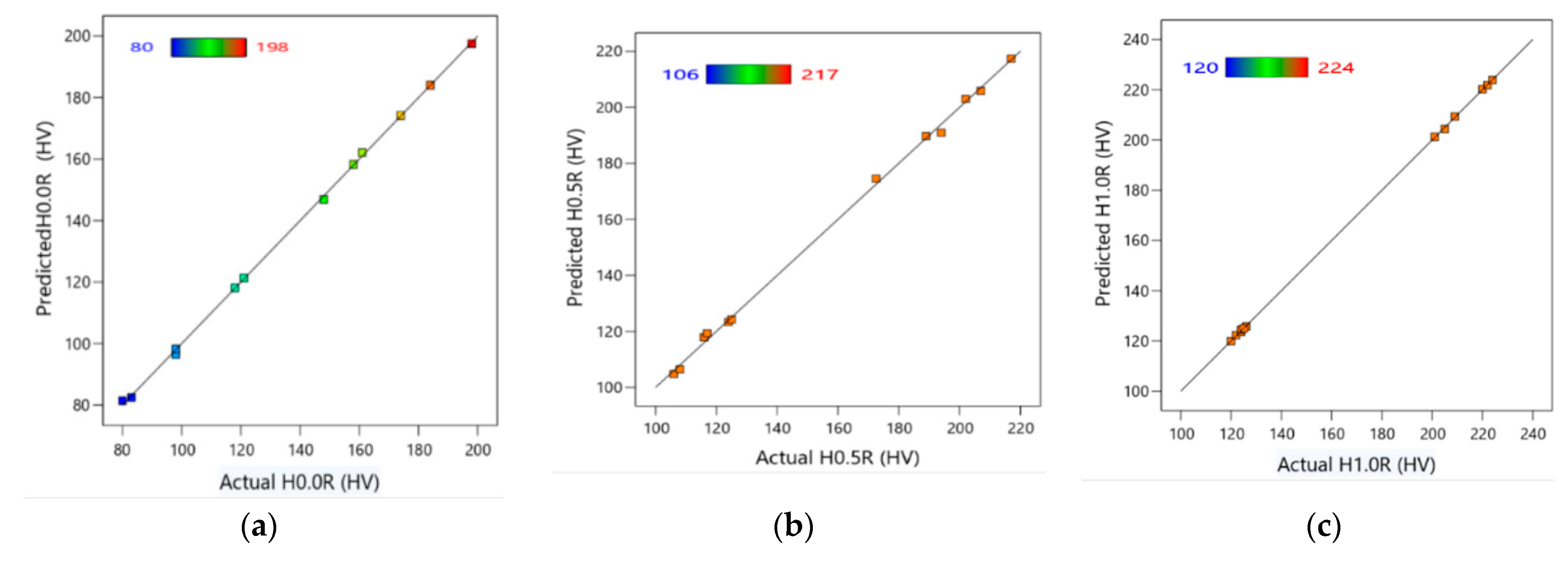
3.3.1. Machine Learning Prediction Models of Hardness Distribution
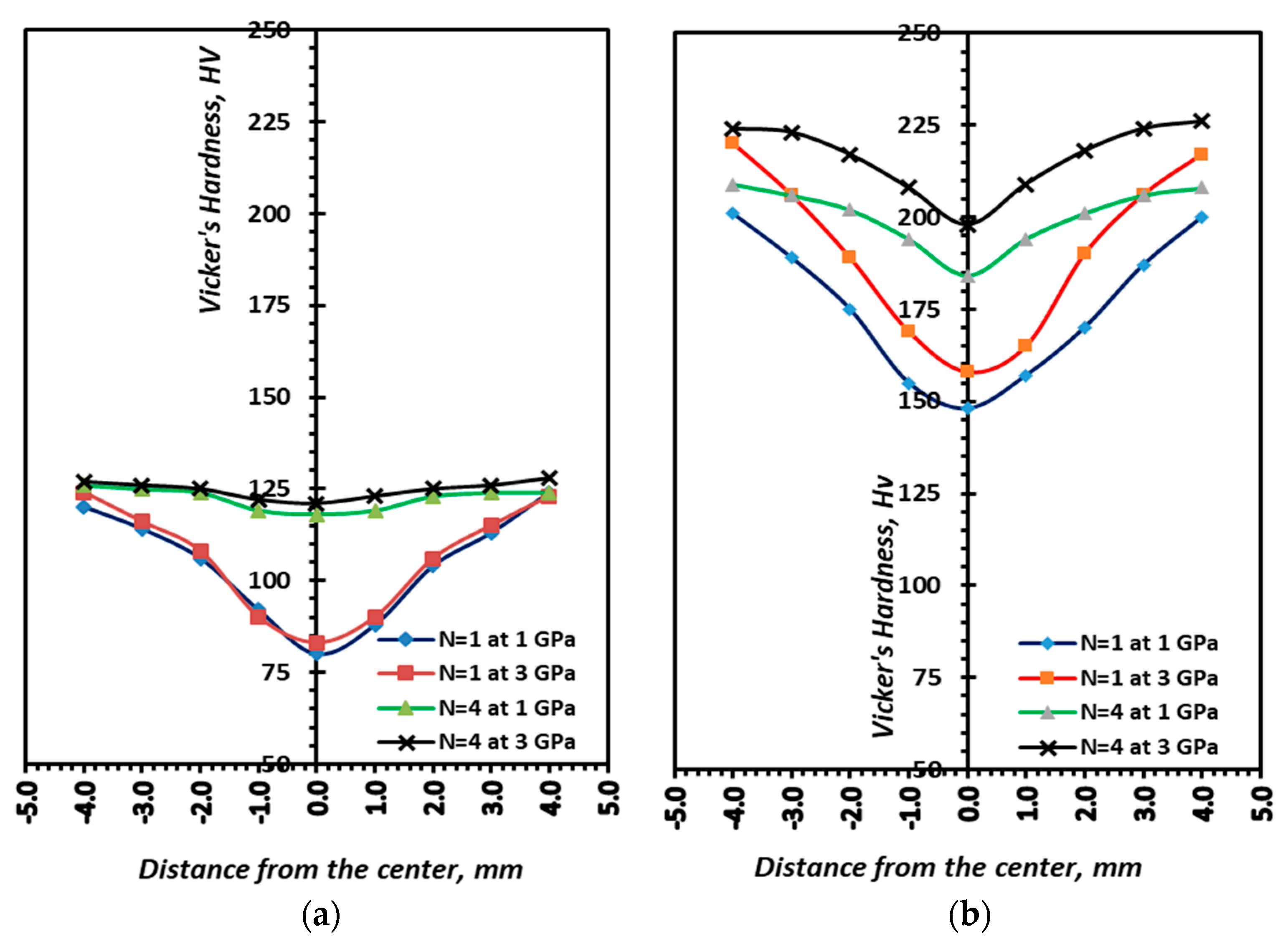
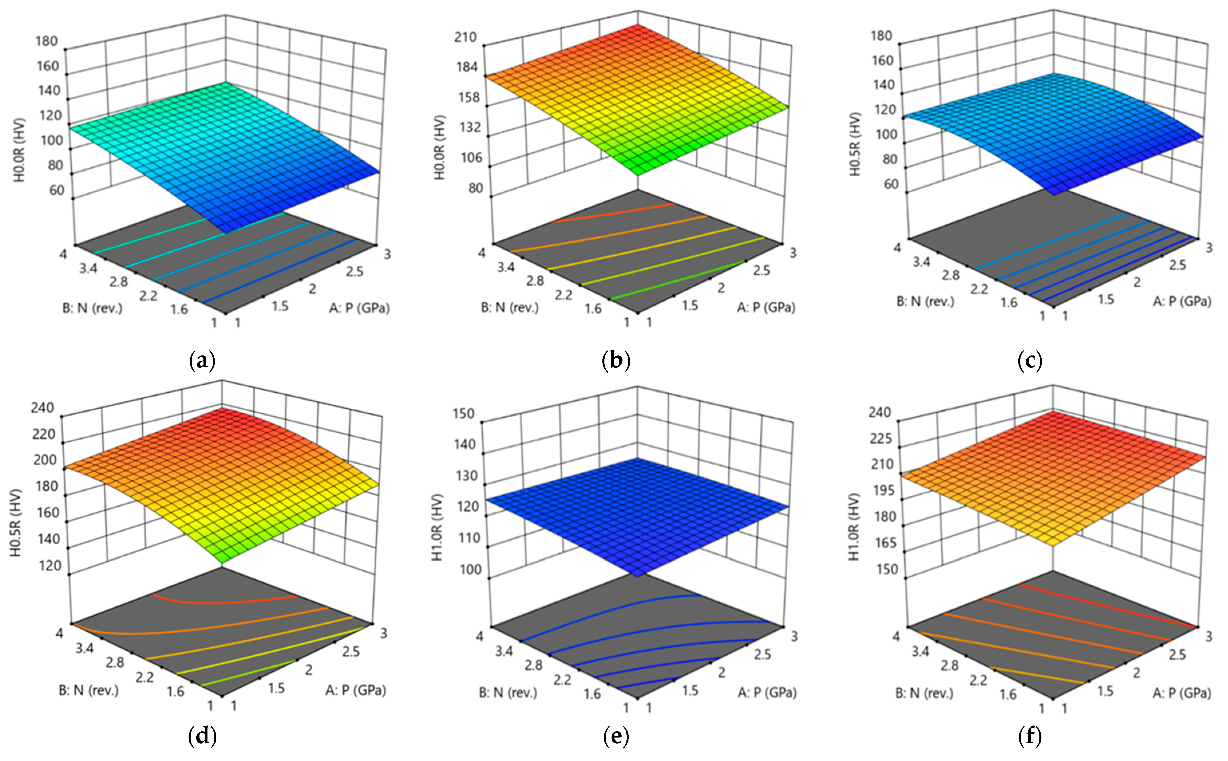
3.3.2. Regression Models and 3D Plots of Hardness Distribution
3.3.3. Optimization of Hardness Distribution
3.4. Compressive Properties
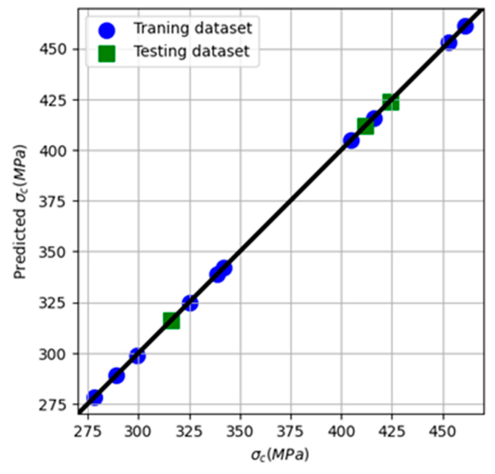
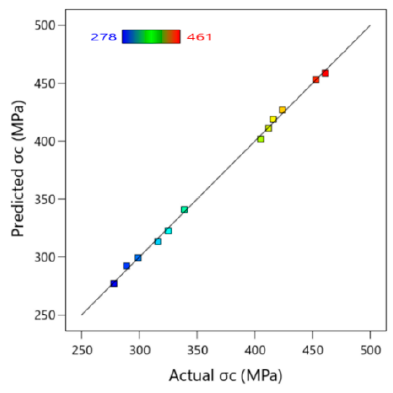
3.4.1. Machine Learning Prediction Models of Compression Properties
3.4.2. Regression Models and 3D Plots of Compression Properties
3.4.3. Optimization of Compression Properties
4. Validation of ML and RSM Models for AA6061 and AA6061/SiCp Processing through HPT
4.1. Validation of ML Model Inferences
4.2. Validation of RSM Models
4.3. Validation of HPT Based on Previous Studies
5. Conclusions
- HPT processing of AA6061/SiCp composite four revolutions at 3 GPa pressures resulted in the refinement of the grain size and sub-grain size by 27% and 46.6%, respectively, compared to the HC counterpart.
- Processing with four revolutions at 3 GPa resulted in improving the hardness and compressive strength of AA6061/SiCp composite by 133% and 34.8%, respectively, compared to the HC counterpart.
- ML results reveals that:
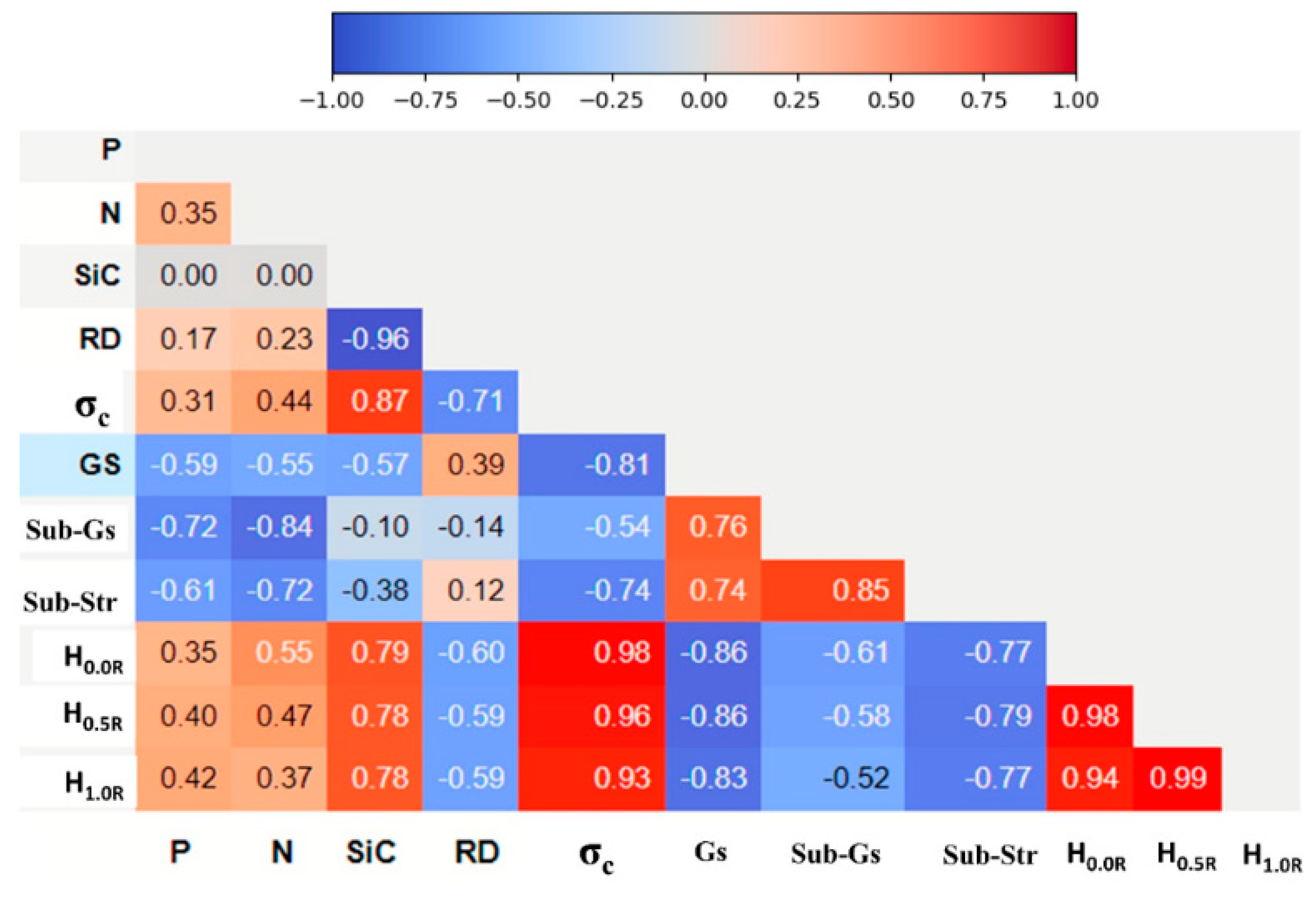
- The correlation plot obtained from ML revealed that SiC content is the most significant parameter in increasing the hardness of AA6061 alloy at H0.0R, H0.5R, H1.0R, and σc of the AA6061 discs with a high positive significant correlation of 0.79, 0.78, 0.78, and 0.87, respectively.
- The correlation plot obtained from ML showed that the GS, Sub-Gs, and Sub-Str were strongly correlated with the number of revolutions of HPT with a high negative significant correlation of −0.55, −0.84, and −0.72, respectively.
- The optimum HPT parameters for AA6061/SiCp composite was four revolutions at 3 GPa.
- Processing the AA6061/SiC composite four revolutions at 3 GPa reduces the grain size and sub-grain size by 27% and 45%, respectively, which resulted in increasing the Vicker’s hardness and compressive strength by 133% and 35%, respectively, compared to the HC counterpart.
- DOE-GA optimization reveals that:
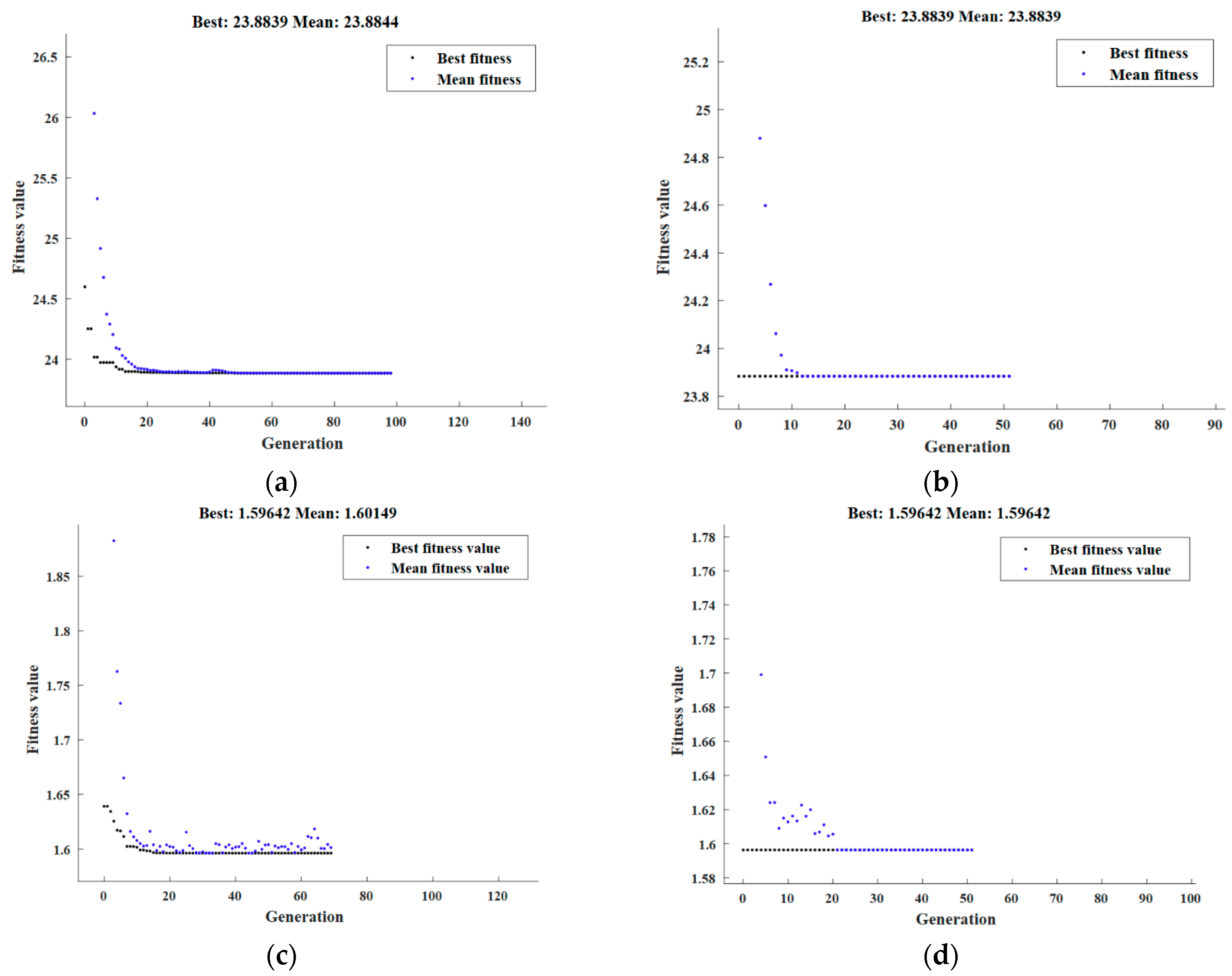
- The minimum GS, Sub-Gs, and Sub-Str were reached at 23.9 µm, 1.6 m, and 154 nm, respectively, with the optimal HPT condition parameters of P = 3 GPa, N = 4 revolutions, and 15% SiC.
- The maximum hardness values at H0.0R, H0.5R, and H1.0R values were calculated to be 197.6 HV, 217.4 HV, and 223.9 HV, respectively, with P = 3 GPa, N = 4 revolutions, and 15% SiC.
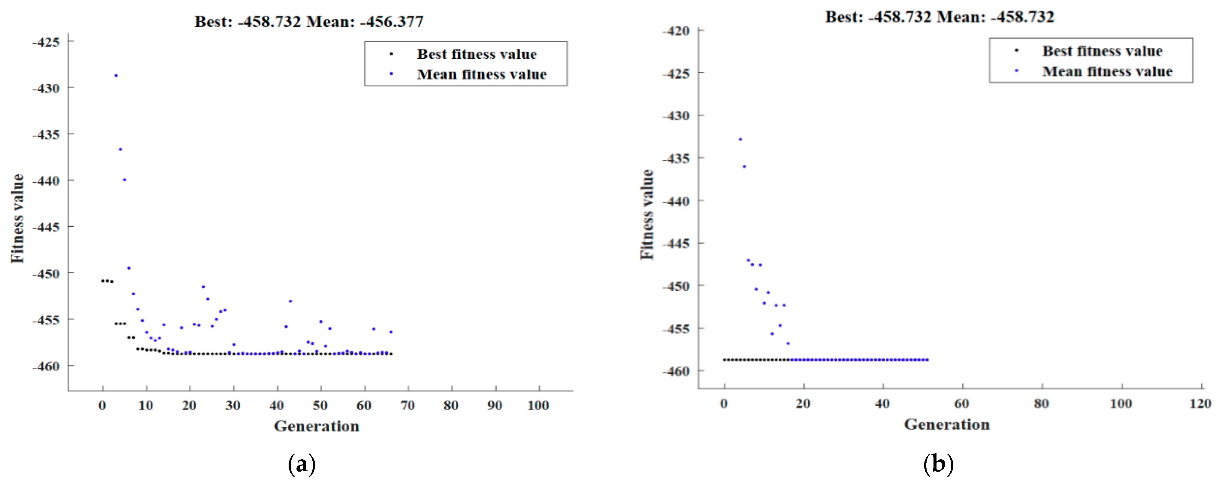
- The maximum σc were reached at 458.7 MPa with the optimal HPT condition parameters of P = 3 GPa, N = 4 revolutions, and 15% SiC.
Author Contributions
Funding
Institutional Review Board Statement
Informed Consent Statement
Data Availability Statement
Acknowledgments
Conflicts of Interest
Appendix A

| Run No. | Input | Output | |||||||||
|---|---|---|---|---|---|---|---|---|---|---|---|
| HPT Conditions | RD (%) | Microstructure | Hardness (HV) | ||||||||
| P (GPa) | N (rev) | SiC% | σc (MPa) | GS (µm) | Sub-Gs (µm) | Sub-Str (nm) | H0.0R | H0.5R | H1.0R | ||
| 1 | as-HC | 0 | 98.5 | 245 | 35 | 3.2 | 610 | 63 | |||
| 2 | as-HC | 15 | 96.4 | 342 | 33 | 3 | 420 | 96 | |||
| 3 | 1 | 1 | 0 | 99.1 | 278 | 33 | 2.8 | 360 | 80 | 106 | 120 |
| 4 | 1 | 2 | 0 | 99.2 | 289 | 31 | 2.5 | 330 | 98 | 116 | 122 |
| 5 | 1 | 4 | 0 | 99.5 | 325 | 30 | 1.9 | 250 | 118 | 124 | 126 |
| 6 | 1 | 1 | 15 | 97.1 | 405 | 31.5 | 2.7 | 260 | 148 | 172.5 | 201 |
| 7 | 1 | 2 | 15 | 97.2 | 416 | 31 | 2.5 | 243 | 161 | 194 | 205 |
| 8 | 1 | 4 | 15 | 97.4 | 453 | 25 | 1.6 | 184 | 184 | 202 | 209 |
| 9 | 3 | 1 | 0 | 99.3 | 299 | 32 | 2 | 277 | 83 | 108 | 124 |
| 10 | 3 | 2 | 0 | 99.3 | 316 | 30.5 | 2 | 270 | 98 | 117 | 124 |
| 11 | 3 | 4 | 0 | 99.5 | 339 | 30 | 1.8 | 240 | 121 | 125 | 125 |
| 12 | 3 | 1 | 15 | 97.1 | 412 | 24.5 | 2.2 | 258 | 158 | 189 | 220 |
| 13 | 3 | 2 | 15 | 97.2 | 424 | 24 | 1.9 | 230 | 174 | 207 | 222 |
| 14 | 3 | 4 | 15 | 97.3 | 461 | 24 | 1.6 | 154 | 198 | 217 | 224 |
| Response | Experimental | RSM | GA | DOE-GA | |
|---|---|---|---|---|---|
| GS | Value | 24 | 23.88 | 23.88 | 23.88 |
| Cond. | 3P, 4 N, 15% | 3P, 4N, 15% | 3P, 4N, 15% | 3P, 4N, 15% | |
| Sub-Gs | Value | 1.6 | 1.6 | 1.6 | 1.6 |
| Cond. | 3P, 4 N, 15% | 3P, 4N, 15% | 3P, 4N, 15% | 3P, 4N, 15% | |
| Sub-Str | Value | 154 | 154 | 1534 | 154 |
| Cond. | 3P, 4N, 15% | 3P, 4N, 15% | 3P, 4N, 15% | 3P, 4N, 15% | |
| RD | Value | 99.5 | 99.5 | 99.5 | 99.5 |
| Cond. | 3P, 4N, 0% | 3P, 4N, 0% | 3P, 4N, 0% | 3P, 4N, 0% | |
| σc | Value | 461 | 458.7 | 458.7 | 458.7 |
| Cond. | 3P, 4N, 15% | 3P, 4N, 15% | 3P, 4N, 15% | 3P, 4N, 15% | |
| H0.0R | Value | 198 | 197.55 | 197.55 | 197.55 |
| Cond. | 3P, 4N, 15% | 3P, 4N, 15% | 3P, 4N, 15% | 3P, 4N, 15% | |
| H0.5R | Value | 217 | 217.38 | 217.38 | 217.38 |
| Cond. | 3P, 4N, 15% | 3P, 4N, 15% | 3P, 4N, 15% | 3P, 4N, 15% | |
| H1.0R | Value | 224 | 223.9 | 223.9 | 223.9 |
| Cond. | 3P, 4N, 15% | 3P, 4N, 15% | 3P, 4N, 15% | 3P, 4N, 15% | |
Appendix B


References
- Flores-Zamora, M.I.; Guel, I.E.; Hernandez, J.G.; Yoshida, M.M.; Sanchez, R.M. Aluminum-graphite composite produced by mechanical milling and hot extrusion. J. Alloys Compd. 2007, 434–435, 518–521. [Google Scholar] [CrossRef]
- Suresha, S.; Sridhara, B.K. Effect of addition of graphite particulates on the wear behavior in aluminum-silicon carbide-graphite composite. Mater. Des. 2010, 31, 1804–1812. [Google Scholar] [CrossRef]
- Suresha, S.; Sridhara, B.K. Wear characteristics of hybrid aluminum matrix composites reinforced with graphite and silicon carbides particulates. Compos. Sci. Technol. 2010, 70, 1652–1659. [Google Scholar] [CrossRef]
- Shorowordi, K.M.; Hasseb, A.S.M.A.; Celis, J.P. Tribo-surface characteristics of Al-B4C and Al-SiC composites worn under different contact pressures. Wear 2006, 261, 634–641. [Google Scholar] [CrossRef]
- Tavakoli, A.H.; Smichi, A.; Reihani, S.M. Study of the compaction behavior of composite powders under monotonic and cyclic loading. Compos. Sci. Technol. 2005, 65, 2094–2104. [Google Scholar] [CrossRef]
- El-Shenawy, M.; Ahmed, M.; Nassef, A.; El-Hadek, M.; Alzahrani, B.; Zedan, Y.; El-Garaihy, W. Effect of ECAP on the Plastic Strain Homogeneity, Microstructural Evolution, Crystallographic Texture and Mechanical Properties of AA2xxx Aluminum Alloy. Metals 2021, 11, 938. [Google Scholar] [CrossRef]
- Salem, H.G.; Sadek, A.A. Fabrication of High-Performance PM Nanocrystalline Bulk AA2124. J. Mater. Eng. Perform. 2009, 19, 356–367. [Google Scholar] [CrossRef] [Green Version]
- Polmear, I.J. Light Alloys-Metallurgy of the Light Metals, 3rd ed.; Arnold: London, UK, 2000. [Google Scholar]
- Salem, H.G.; El-Garaihy, W.H.; Al-Rassoul, E.S.M. Influence of high-pressure torsion on the consolidation behavior and mechanical properties of AA6061-SiCp composite powders. In Supplemental Proceedings; John Wiley & Sons, Ltd.: Hoboken, NJ, USA, 2012; pp. 553–560. [Google Scholar] [CrossRef]
- Alateyah, A.I.; Alawad, M.O.; Aljohani, T.A.; El-Garaihy, W.H. Effect of ECAP Route Type on the Microstructural Evolution, Crystallographic Texture, Electrochemical Behavior and Mechanical Properties of ZK30 Biodegradable Magnesium Alloy. Materials 2022, 15, 6088. [Google Scholar] [CrossRef]
- Zhilyaev, A.P.; Langdon, T.G. Using high-pressure torsion for metal processing: Fundamentals and applications. Prog. Mater. Sci. 2008, 53, 893–979. [Google Scholar] [CrossRef]
- El-Garaihy, W.H.; Fouad, D.M.; Salem, H.G. Multi-channel Spiral Twist Extrusion (MCSTE): A Novel Severe Plastic Defor-mation Technique for Grain Refinement. Met. Mater. Trans. A 2018, 49, 2854–2864. [Google Scholar] [CrossRef]
- Zhilyaev, A.P.; Nurislamova, G.V.; Kim, B.K.; Baró, M.D.; Szpunar, J.A.; Langdon, T.G. Experimental parameters influencing grain refinement and microstructural evolution during high-pressure torsion. Acta Mater. 2003, 51, 753–765. [Google Scholar] [CrossRef]
- Jiang, H.; Zhu, Y.T.; Butt, D.P.; Alexandrov, I.V.; Lowe, T.C. Microstructural evolution, microhardness and thermal stability of HPT-processed Cu. Mater. Sci. Eng. A 2000, 290, 128–138. [Google Scholar] [CrossRef]
- El Aal, M.I.A. The influence of ECAP and HPT processing on the microstructure evolution, mechanical properties and tribology characteristics of an Al6061 alloy. J. Mater. Res. Technol. 2020, 9, 12525–12546. [Google Scholar] [CrossRef]
- El Aal, M.I.A. Recycling of Al chips and Al chips composites using high-pressure torsion. Mater. Res. Express 2021, 8, 056514. [Google Scholar] [CrossRef]
- Deng, N.T.G.; Zhao, X.; Su, L.; Wei, P.; Zhang, L.; Zhan, L.; Chong, Y.; Zhu, H. Effect of high-pressure torsion process on the microhardness, microstructure and tribological property of Ti6Al4V alloy. J. Mater. Sci. Technol. 2021, 94, 183–195. [Google Scholar] [CrossRef]
- Edalati, K.; Akiba, E.; Horita, Z. High-pressure torsion for new hydrogen storage materials. Sci. Technol. Adv. Mater. 2018, 19, 185–193. [Google Scholar] [CrossRef]
- Schmidt, J.; Marques, M.R.; Botti, S.; Marques, M.A. Recent advances and applications of machine learning in solid-state materials science. Npj Comput. Mater. 2019, 5, 83. [Google Scholar] [CrossRef] [Green Version]
- Wen, C.; Zhang, Y.; Wang, C.; Xue, D.; Bai, Y.; Antonov, S.; Dai, L.; Lookman, T.; Su, Y. Machine learning assisted design of high entropy alloys with desired property. Acta Mater. 2019, 170, 109–117. [Google Scholar] [CrossRef] [Green Version]
- Butler, K.T.; Davies, D.W.; Cartwright, H.; Isayev, O.; Walsh, A. Machine learning for molecular and materials science. Nature 2018, 559, 547–555. [Google Scholar] [CrossRef] [Green Version]
- Shaban, M.; Alateyah, A.I.; Alsharekh, M.F.; Alawad, M.O.; BaQais, A.; Kamel, M.; Alsunaydih, F.N.; El-Garaihy, W.H.; Salem, H.G. Influence of ECAP Parameters on the Structural, Electrochemical and Mechanical Behavior of ZK30: A Combination of Experimental and Machine Learning Approaches. J. Manuf. Mater. Process. 2023, 7, 52. [Google Scholar] [CrossRef]
- Schleder, G.R.; Padilha, A.C.M.; Acosta, C.M.; Costa, M.; Fazzio, A. From DFT to machine learning: Recent approaches to materials science—A review. J. Phys. Mater. 2019, 2, 032001. [Google Scholar]
- Wang, A.Y.T.; Murdock, R.J.; Kauwe, S.K.; Oliynyk, A.O.; Gurlo, A.; Brgoch, J.; Persson, K.A.; Sparks, T.D. Machine learning for materials scientists: An introductory guide toward best practices. Chem. Mater. 2020, 32, 4954–4965. [Google Scholar]
- Ghaedi, M.; Azad, F.N.; Dashtian, K.; Hajati, S.; Goudarzi, A.; Soylak, M. Central composite design and genetic algorithm applied for the optimization of ultrasonic-assisted removal of malachite green by ZnO Nanorod-loaded activated carbon. Spectrochim. Acta Part A Mol. Biomol. Spectrosc. 2016, 167, 157–164. [Google Scholar] [CrossRef]
- Dadrasi, A.; Fooladpanjeh, S.; Gharahbagh, A.A. Interactions between HA/GO/epoxy resin nanocomposites: Optimization, modeling and mechanical performance using central composite design and genetic algorithm. J. Braz. Soc. Mech. Sci. Eng. 2019, 41, 41–63. [Google Scholar]
- Santhosh, A.J.; Tura, A.D.; Jiregna, I.T.; Gemechu, W.F.; Ashok, N.; Ponnusamy, M. Optimization of CNC turning parameters using face centred CCD approach in RSM and ANN-genetic algorithm for AISI 4340 alloy steel. Results Eng. 2021, 11, 100251. [Google Scholar] [CrossRef]
- Sarker, I.H. Machine learning: Algorithms, real-world applications and research directions. SN Comput. Sci. 2021, 2, 160. [Google Scholar]
- Williams, C.K.; Rasmussen, C.E. Gaussian Processes for Machine Learning; MIT Press: Cambridge, MA, USA, 2006. [Google Scholar]
- Deringer, V.L.; Bartók, A.P.; Bernstein, N.; Wilkins, D.M.; Ceriotti, M.; Csányi, G. Gaussian process regression for materials and molecules. Chem. Rev. 2021, 121, 10073–10141. [Google Scholar]
- Vapnik, V. The Nature of Statistical Learning Theory; Springer Science & Business Media: New York, NY, USA, 1999. [Google Scholar]
- Cherkassky, V.; Ma, Y. Practical selection of SVM parameters and noise estimation for SVM regression. Neural Netw. 2014, 17, 113–126. [Google Scholar] [CrossRef] [Green Version]
- Ahmad, A.S.; Hassan, M.Y.; Abdullah, M.P.; Rahman, H.A.; Hussin, F.; Abdullah, H.; Saidur, R. A review on applications of ANN and SVM for building electrical energy consumption forecasting. Renew. Sustain. Energy Rev. 2014, 33, 102–109. [Google Scholar]
- Blanco, V.; Japón, A.; Puerto, J. A mathematical programming approach to SVM-based classification with label noise. Comput. Ind. Eng. 2022, 172, 108611. [Google Scholar]
- Ahmed, N.I.; Nasrin, F. Reducing Error Rate for Eye-Tracking System by Applying SVM. In Machine Intelligence and Data Science Applications; Springer: New York, NY, USA, 2022; pp. 35–47. [Google Scholar]
- Hazir, E.; Ozcan, T. Response surface methodology integrated with desirability function and genetic algorithm approach for the optimization of CNC machining parameters. Arab. J. Sci. Eng. 2019, 44, 2795–2809. [Google Scholar] [CrossRef]
- Bidulska, J.; Kocisko, R.; Bidulsky, R.; Grande, A.; Donic, T.; Martikan, M. Effect of severe plastic deformation on the porosity characteristics of Al-Zn-Mg-Cu PM alloy. Acta Metall. Slovaca 2010, 16, 4–11. [Google Scholar]
- Stolyarov, V.V.; Zhu, Y.T.; Lowe, T.C.; Islamgalive, R.K.; Valiev, R.Z. Processing nanocrystalline Ti and its nanocomposites from micrometer-sized Ti powder using high pressure torsion. Mater. Sci. Eng. A 2000, 282, 78–85. [Google Scholar] [CrossRef]
- Langdon, T.G. The significance of strain reversals during processing by high-pressure torsion. Mater. Sci. Eng. A 2008, 498, 341–348. [Google Scholar] [CrossRef]
- Langdon, T.G.; Xu, C. Three-dimensional representations of hardness distributions after processing by high-pressure torsion. Mater. Sci. Eng. A 2009, 503, 71–74. [Google Scholar] [CrossRef]
- Langdon, T.G.; Xu, C.; Horita, Z. The evolution of homogeneity in an aluminum alloy processed using high-pressure torsion. Acta Mater. 2008, 56, 5168–5176. [Google Scholar] [CrossRef]
- Estrin, Y.; Molotnikov, A.; Davies, C.H.; Lapovok, R. Strain gradient plasticity modelling of high-pressure torsion. J. Mech. Phys. Solids 2008, 56, 1186–1202. [Google Scholar] [CrossRef]
- Moreno-Valle, E.C.; Sabirov, I.; Perez-Prado, M.T.; Murashkin, M.Y.; Bobruk, E.V.; Valiev, R.Z. Effect of the grain refinement via severe plastic deformation on strength properties and deformation behavior of an Al6061 alloy at room and cryogenic temperatures. Mater. Lett. 2011, 65, 2917–2919. [Google Scholar]
- Wetscher, F.; Vorhauer, A.; Pippan, R. Strain hardening during high pressure torsion deformation. Mater. Sci. Eng. A 2005, 410–411, 213–216. [Google Scholar] [CrossRef]
- Valiev, R.Z.; Rovan, H.J.; Liu, M.; Murashkin, M.; Kilmametov, A.R.; Ungar, T.; Balogh, L. Nanostructures and Microhardness in Al and Al–Mg Alloys Subjected to SPD. Mater. Sci. Forum 2009, 604–605, 179–185. [Google Scholar] [CrossRef]
- Alateyah, A.I.; Alawad, M.O.; Aljohani, T.A.; El-Garaihy, W.H. Influence of Ultrafine-Grained Microstructure and Texture Evolution of ECAPed ZK30 Magnesium Alloy on the Corrosion Behavior in Different Corrosive Agents. Materials 2022, 15, 5515. [Google Scholar] [CrossRef] [PubMed]
- Borodachenkova, M.; Wen, W.; de Bastos Pereira, A.M. High-Pressure Torsion: Experiments and Modeling. In Severe Plastic Deformation Techniques; Licensee IntechOpen: London, UK, 2017; pp. 93–112. [Google Scholar]


| Response | F-Value | Model Significance (p < 0.05) | Adeq Precision (Ratio > 4) | R2 | R2adj | R2pred |
|---|---|---|---|---|---|---|
| RD | 2946.48 | <0.0001 | 114.5568 | 0.9997 | 0.9994 | 0.9983 |
| GS | 221.95 | <0.0001 | 38.5169 | 0.9942 | 0.9897 | 0.9815 |
| Sub-Gs | 52.16 | 0.0002 | 20.3463 | 0.9843 | 0.9654 | 0.9255 |
| Sub-Str | 1.885 × 10⁵ | 0.0018 | 1609.9703 | 1.0000 | 1.0000 | 0.9998 |
| H0.0R | 1382.99 | <0.0001 | 103.7168 | 0.9996 | 0.9989 | 0.9967 |
| H0.5R | 399.68 | <0.0001 | 50.2033 | 0.9986 | 0.9961 | 0.9894 |
| H1.0R | 11,784.14 | <0.0001 | 232.2409 | 1.0000 | 0.9999 | 0.9996 |
| σc | 650.50 | <0.0001 | 67.0922 | 0.9987 | 0.9972 | 0.9902 |
| Parameter | ML Algorithm | Training Set | Testing Set | ||
|---|---|---|---|---|---|
| RMSE | R2 | RMSE | R2 | ||
| RD (%) | LR | 0.148 | 0.98 | 0.119 | 0.98 |
| GPR | 0.184 | 0.97 | 0.182 | 0.96 | |
| SVR | 0.195 | 0.97 | 0.130 | 0.98 | |
| Parameter | ML Algorithm | Training Set | Testing Set | ||
|---|---|---|---|---|---|
| RMSE | R2 | RMSE | R2 | ||
| GS (µm) | LR | 1.50 | 0.74 | 1.57 | 0.88 |
| GPR | 0.59 | 0.96 | 0.61 | 0.98 | |
| SVR | 0.05 | 0.99 | 0.05 | 0.99 | |
| Sub-Gs (µm) | LR | 0.17 | 0.88 | 1.57 | 0.88 |
| GPR | 0.03 | 0.99 | 0.61 | 0.98 | |
| SVR | 0.05 | 0.99 | 0.05 | 0.99 | |
| Sub-Str (nm) | LR | 39.38 | 0.73 | 62.76 | 0.84 |
| GPR | 11.47 | 0.98 | 14.74 | 0.99 | |
| SVR | 0.51 | 0.99 | 8.48 | 0.99 | |
| Parameter (HV) | The Optimized Model Achieved Using | Training Set | Testing Set | ||
|---|---|---|---|---|---|
| RMSE | R2 | RMSE | R2 | ||
| H0.0R | LR | 9.42 | 0.94 | 6.03 | 0.98 |
| GPR | 7.51 | 0.96 | 6.31 | 0.98 | |
| SVM | 0.05 | 0.99 | 0.05 | 0.99 | |
| H0.5R | LR | 18.45 | 0.82 | 6.23 | 0.99 |
| GPR | 8.60 | 0.96 | 7.34 | 0.98 | |
| SVR | 0.05 | 0.99 | 0.05 | 0.99 | |
| H1.0R | LR | 18.45 | 0.82 | 6.23 | 0.98 |
| GPR | 8.60 | 0.96 | 7.34 | 0.98 | |
| SVR | 3.35 | 0.99 | 5.97 | 0.99 | |
| Parameter (MPa) | ML Algorithm | Training Set | Testing Set | ||
|---|---|---|---|---|---|
| RMSE | R2 | RMSE | R2 | ||
| σc | LR | 9.48 | 0.98 | 2.58 | 0.99 |
| GPR | 13.64 | 0.96 | 9.61 | 0.98 | |
| SVR | 0.05 | 0.99 | 4.24 | 0.99 | |
| Response | SiC % | Experimental | Validation | Error % | Accuracy |
|---|---|---|---|---|---|
| RD | 0 | 99.33 | 99.43 | −0.1 | 99.90% |
| 15 | 97.35 | 97.33 | 0.02 | 99.98% | |
| GS (µm) | 0 | 30.4 | 30.02 | 1.25 | 98.75% |
| 15 | 26 | 28.23 | −8.58 | 91.42% | |
| Sub-Gs (µm) | 0 | 2.2 | 2.18 | 0.91 | 99.09% |
| 15 | 2 | 2.01 | −0.5 | 99.50% | |
| Sub-Str (nm) | 0 | 295 | 286.89 | 2.75 | 97.25% |
| 15 | 225 | 243.21 | −8.09 | 91.91% | |
| H0.0R | 0 | 105 | 127.14 | −21.09 | 78.91% |
| 15 | 172 | 127.15 | 26.08 | 73.92% | |
| H0.5R | 0 | 120 | 145.46 | −21.22 | 78.78% |
| 15 | 198 | 145.47 | 26.53 | 73.47% | |
| H1.0R | 0 | 125 | 155.78 | −24.62 | 75.38% |
| 15 | 206 | 155.79 | 24.37 | 75.63% | |
| σc | 0 | 296 | 357.43 | −20.75 | 79.25% |
| 15 | 428 | 357.43 | 16.49 | 83.51% |
| Response | SiC % | Experimental | Validation | Error % | Accuracy |
|---|---|---|---|---|---|
| GS (µm) | 0 | 30.4 | 30.39 | 0.03 | 99.97% |
| 15 | 26 | 28.44 | −9.38 | 90.62% | |
| Sub-Gs (µm) | 0 | 2.2 | 2.21 | −0.45 | 99.55% |
| 15 | 2 | 1.96 | 2.00 | 98.00% | |
| Sub-Str (nm) | 0 | 295 | 293.39 | 0.54 | 99.46% |
| 15 | 225 | 217.61 | 3.28 | 96.72% | |
| RD (%) | 0 | 99.33 | 99.35 | −0.02 | 99.98% |
| 15 | 97.35 | 97.26 | 0.09 | 99.91% | |
| σc (MPa) | 0 | 296 | 307.46 | −3.87 | 96.13% |
| 15 | 428 | 436.11 | −1.89 | 98.11% | |
| H0.0R | 0 | 105 | 108.71 | −3.53 | 96.47% |
| 15 | 172 | 174.47 | −1.44 | 98.56% | |
| H0.5R | 0 | 120 | 124.08 | −3.40 | 96.40% |
| 15 | 198 | 200.44 | −1.23 | 98.77% | |
| H1.0R | 0 | 125 | 124.24 | 0.61 | 99.39% |
| 15 | 206 | 207.07 | −0.05 | 99.95% |
| Response | GA | DOE-GA | |
|---|---|---|---|
| GS (µm) | Value | 0.54457 | 0.54457 |
| Cond. | 1P, 8N, 15% | 1P, 8N, 15% | |
| Sub-Gs (µm) | Value | 0.0607119 | 0.0607117 |
| Cond. | 1P, 8N, 15% | 1P, 8N, 15% | |
| Sub-Str (nm) | Value | 50.9109 | 50.9109 |
| Cond. | 3P, 6N, 15% | 3P, 6N, 15% | |
| RD (%) | Value | 100.473 | 100.473 |
| Cond. | 1P, 12N, 0% | 1P, 12N, 0% | |
| σc (MPa) | Value | 587.623 | 587.623 |
| Cond. | 1P, 12N, 15% | 1P, 12N, 15% | |
| H0.0R | Value | 211.333 | 211.333 |
| Cond. | 3P, 7N, 15% | 3P, 7N, 15% | |
| H0.5R | Value | 217.375 | 217.375 |
| Cond. | 3P, 4N, 15% | 3P, 4N, 15% | |
| H1.0R | Value | 224.298 | 224.298 |
| Cond. | 3P, 5N, 15% | 3P, 5N, 15% | |
Disclaimer/Publisher’s Note: The statements, opinions and data contained in all publications are solely those of the individual author(s) and contributor(s) and not of MDPI and/or the editor(s). MDPI and/or the editor(s) disclaim responsibility for any injury to people or property resulting from any ideas, methods, instructions or products referred to in the content. |
© 2023 by the authors. Licensee MDPI, Basel, Switzerland. This article is an open access article distributed under the terms and conditions of the Creative Commons Attribution (CC BY) license (https://creativecommons.org/licenses/by/4.0/).
Share and Cite
El-Garaihy, W.H.; Alateyah, A.I.; Shaban, M.; Alsharekh, M.F.; Alsunaydih, F.N.; El-Sanabary, S.; Kouta, H.; El-Taybany, Y.; Salem, H.G. A Comparative Study of a Machine Learning Approach and Response Surface Methodology for Optimizing the HPT Processing Parameters of AA6061/SiCp Composites. J. Manuf. Mater. Process. 2023, 7, 148. https://doi.org/10.3390/jmmp7040148
El-Garaihy WH, Alateyah AI, Shaban M, Alsharekh MF, Alsunaydih FN, El-Sanabary S, Kouta H, El-Taybany Y, Salem HG. A Comparative Study of a Machine Learning Approach and Response Surface Methodology for Optimizing the HPT Processing Parameters of AA6061/SiCp Composites. Journal of Manufacturing and Materials Processing. 2023; 7(4):148. https://doi.org/10.3390/jmmp7040148
Chicago/Turabian StyleEl-Garaihy, Waleed H., Abdulrahman I. Alateyah, Mahmoud Shaban, Mohammed F. Alsharekh, Fahad Nasser Alsunaydih, Samar El-Sanabary, Hanan Kouta, Yasmine El-Taybany, and Hanadi G. Salem. 2023. "A Comparative Study of a Machine Learning Approach and Response Surface Methodology for Optimizing the HPT Processing Parameters of AA6061/SiCp Composites" Journal of Manufacturing and Materials Processing 7, no. 4: 148. https://doi.org/10.3390/jmmp7040148