A Ray Tracing Model for Electron Optical Imaging in Electron Beam Powder Bed Fusion

Abstract

The recent success of the process monitoring method Electron Optical Imaging, applied in the additive manufacturing process Electron Beam Powder Bed Fusion, necessitates a clear understanding of the underlying image formation process. Newly developed multi-detector systems enable the reconstruction of the build surface topography in-situ but add complexity to the method. This work presents a physically based raytracing model, which rationalises the effect of detector positioning on image contrast development and masking. The model correctly describes the effect of multiple scattering events on vacuum chamber walls or heat shields and represents, therefore, a predictive tool for designing future detector systems. Most importantly, this work provides a validated method to compute build surface height gradients directly from experimentally recorded electron-optical images of a multi-detector system without any calibration steps. The computed surface height gradients can be used subsequently as input of normal integration algorithms aiming at the in-situ reconstruction of the build surface topography.

1. Introduction

Additive manufacturing (AM) is driving innovation in many fields of engineering and technology; application examples range from new types of heat exchangers [1] to space applications [2,3]. However, additively manufactured parts intended for components in high-risk/high-value constructions are difficult to develop without extensive trial and error phases. In addition, the qualification of these parts is still a major challenge for all stakeholders along the various value chains. In-situ, layer-based process monitoring provides the possibility to accelerate process parameter development for new materials or potentially the development of part-specific parameters. Accurate defect detection allows us to implement correction strategies or even to qualify to build parts and to replace traditional non-destructive evaluation techniques [4].

Recently, Electron optical (ELO) imaging has been demonstrated to be a successful, reliable process monitoring method in electron beam powder bed fusion (PBF-EB), which has been used to develop process parameters [5], defection detection [6] or the assessment of dimensional accuracy [7]. After melting, the solidified build surface is scanned in a separate additional process step with a focused and low-power electron beam. Then, an image is reconstructed from 1D voltage time series data recorded by appropriate detector systems, similar to the scanning electron microscope (SEM). This allows one to inspect the melt surfaces of parts for defects such as surface bulging or surface porosity in-situ during the build process every layer of a part. Single detectors systems are placed either directly in the beam-column and coaxially to the incoming beam [5], get integrated into heat shields [8] or just attached to the vacuum chamber ceiling [9].

Multi-detector systems were newly developed, which allow harvesting topographical and material contrast information from the build surface [9,10]. A multi-detector system comprised of four single detectors is presented in a previous publication [11]. The integral part of this work is the in-situ measurement of the surface height gradient $\nabla \overline{Z}(x,y)$, which approximates the true height gradient $\nabla Z(x,y)$ of the true build surface height $Z(x,y)$. Various correction and calibration steps are necessary to obtain the gradient, beginning with surface tilt and solid angle (STSA) contrast correction. Surface tilt contrast is a distortion effect that develops in ELO images due to the special geometrical conditions of single and multi-detector systems inside PBF-EB machines. The effect can be corrected simply by normalizing ELO images recorded in situ during the process with images recorded from a calibration plate. The basis for the computation of the measure $\nabla \overline{Z}(x,y)$ are STSA contrast corrected normalised difference images. They are obtained by computing the difference divided by the sum of the ELO images recorded by opposite detectors. After further computation and calibration steps, it becomes possible to reconstruct the build surface topography using existing normal integration algorithms.

The described variety of investigated detector systems necessitates a solid understanding of ELO image formation to realise the full potential of multi-detector systems. This work builds on a simplified model of ELO image formation [11] and extends it to include multiple scattering events at the vacuum chamber interior. Commonly, the SEM community uses Monte Carlo models to study the interaction of electron beams with the surface under investigation [12]. However, following the trajectory of single, possibly interacting, electron pathways below the imaged surface is not useful in the context of ELO imaging. For example, the special geometric conditions of a PBF-EB machine (small, distant detectors and big imaging areas) determine the later image but depend only on the emitted electrons. Additionally, typical beam currents are in the order of $\mathrm{m}\mathrm{A}$, which means Monte Carlo models for ELO imaging might be computationally more demanding than similar models used in SEM. Therefore, the ELO image formation process is modelled in the spirit of classical ray tracing algorithms by incorporating known phenomenological descriptions of electron scattering.

The overall aim of this work is to enhance the process monitoring method ELO imaging by providing a physically based model of the imaging process itself. A special focus is placed on multi-detector systems, which promise additional, previously unknown, insights into PBF-EB. The provided model equations are validated with experimental ELO images recorded by a multi-detector system. Detector positioning has a strong effect on the image formation, and influences contrast development and masking. Masking develops when obstacles in the pathway of scattered electrons prevent them from hitting a detector. This is a deeply unwanted effect for gradient computation in the context of surface topography reconstruction and can be understood by the interplay of the developing scattering function, the local surface normal vector, and detector positioning. Most significantly, this work shows that STSA correction introduces a position-dependent distortion in the normalised difference images $M_x$ and $M_y$. A new equation is developed, which allows one to compute $\nabla \overline{Z}(x,y)$ directly from four ELO images without any distortion effects or previously necessary calibration steps. This is a significant improvement to the previous study [11] and is enabled by the theoretical insights of this work.

2. Materials and Methods

The ELO ray tracing model is developed in the following. It builds on a simplified model of ELO image formation [11], which includes only the first scattering event of the primary beam electrons with the build surface. This extension provides additional equations, which allow one to compute the influence of multiple scattering events on image formation. Further, a validation experiment is described, and the simulation set-ups are used in this work.

2.1. ELO Ray Tracing Model

Physically, the electron beam scans over the build surfaces in a square line-by-line pattern of width w (see Figure 1a) with a defined scan velocity $v_s$ and beam current $I_b$. The electron beam is fully described by the positions and momenta of all electrons forming it. Geometrically, the beam is a 3D object showing a caustic along its elongated direction. The beam forms a 2D power density distribution at the intersection with the build surface, which is called the beam profile. The shape and size of the beam profile will vary upon deflection by the angle $\varphi$. The characteristics of the beam profile are highly significant for ELO imaging since imaging a surface with electrons by scanning is mathematically described by the convolution of the beam profile with the surface [13]. Commonly, the 2D power density distribution is simplified to a single scalar value, the beam diameter. Single primary electrons (PE) can enter the build surface either on locations of parts or of sintered powder. Either way, PE experiences a variety of interactions with the material. Elastic interactions of electrons with the atomic nuclei give rise to the emission of back scattered electrons (BSE), which are electrons defined to have kinetic energies >$50 \mathrm{e}\mathrm{V}$. Averaging over all primary beam electron trajectories inside the solid forms the information volume. Its intersection with the build surface extends the spatial dimension of the beam current distribution and influences, therefore, the imaging process. Inelastic interactions of PE with the atoms of part or powder give rise to the ejection of weakly bound shell electrons, which are then emitted as secondary electrons (SE). They posses low kinetic energies, by definition <$50 \mathrm{e}\mathrm{V}$, due to their generation process. More details on the origin of BSE and the generation of SE and further electron-material interactions are summarised in [14,15].

The general probability density function $f(E,\theta ,A,E_B,d\Omega )$ describes the probability of finding an emitted/backscattered electron inside the solid angle element $d\Omega$ with the energy $E_B$. Originally, the electron escaped from a local surface element consisting of atoms with the atomic number A and was described by the local surface normal vector ${\overrightarrow{n}}_S$. It was generated by PE (of the electron beam), which hit the local surface element with an energy E in the direction ${\overrightarrow{p}}_E$. The vectors ${\overrightarrow{n}}_S$ and ${\overrightarrow{p}}_E$ form the angle $\theta$ as illustrated in Figure 1b, if ${\overrightarrow{n}}_S$ is parallel to the the z-axis then $\theta =\varphi$ (see Figure 1a).

The general scattering function $g(E,\theta ,A,d\Omega )$ describes the probability of finding an electron inside the solid angle element $d\Omega$, it is defined by the integral of f over all electron energies $E_B$. For example, the scattering function $g_{\mathrm{BSE}}$ specific to BSE is obtained by

$$g_{\mathrm{BSE}}(E,\theta ,A,d\Omega )={\int }_{50\mathrm{e}\mathrm{V}}^{E}f(E,\theta ,A,E_B,d\Omega )d{E}_{\mathrm{B}}.$$

(1)

The BSE coefficient $\eta (E,\theta ,A)$ can be measured experimentally as the quotient of the number of BSE $N_{\mathrm{BSE}}$ and the number of PE $N_0$. It is defined by the integral of $g_{\mathrm{BSE}}$ over the solid angle of the hemisphere ${\Omega }_{\mathrm{HS}}$ above the interaction point as

$$\eta (E,\theta ,A)={\int }_{{\Omega }_{\mathrm{HS}}}{g}_{\mathrm{BSE}}(E,\theta ,A,d\Omega )d\Omega =\frac{N_{\mathrm{BSE}}}{N_0}.$$

(2)

Reversely, $\eta$ can be used to define $g_{\mathrm{BSE}}=d\eta /d\Omega$ and $f=d^2\eta /d{E}_{B}d\Omega$. The above treatment follows Reimer [16] and is adapted to the present context.

The scattering function describing SE and the respective coefficient can be found in the same way, but SE are neglected in the current form of the model for reasons which are described in detail in Appendix B.

ELO imaging uses robust detector set-ups made of conducting metal plates to cope with the harsh conditions during a build [8,9,10,11]. Ledford et al. [9] argue that these detector designs are sensitive to BSE, SE, Auger electrons and additionally to charge transfer inducing phenomena such as ionised shielding gas, plasma, thermionic emission or just charged and ejected powder particles. For example, inert gases such as helium are frequently used to improve image quality [5,8]. These effects are neglected since implementable phenomenological equations are missing, and the relative importance of the effects is unknown.

Therefore, in summary, only BSE contributes to the charge measured at the detector plates. Furthermore, it is assumed that the detector plates integrate all incoming electrons, and backscattering at the detector plates themselves is neglected. While it is easily possible to implement the effect in the model below, it is unclear how to validate it isolated. In addition, possible influences of the detector material or detector temperature on the measurement chain are ignored. The energy distribution of BSE is not considered, which means all BSE moves instantaneously from the build surface to the detector. Further simplifications are mentioned when necessary.

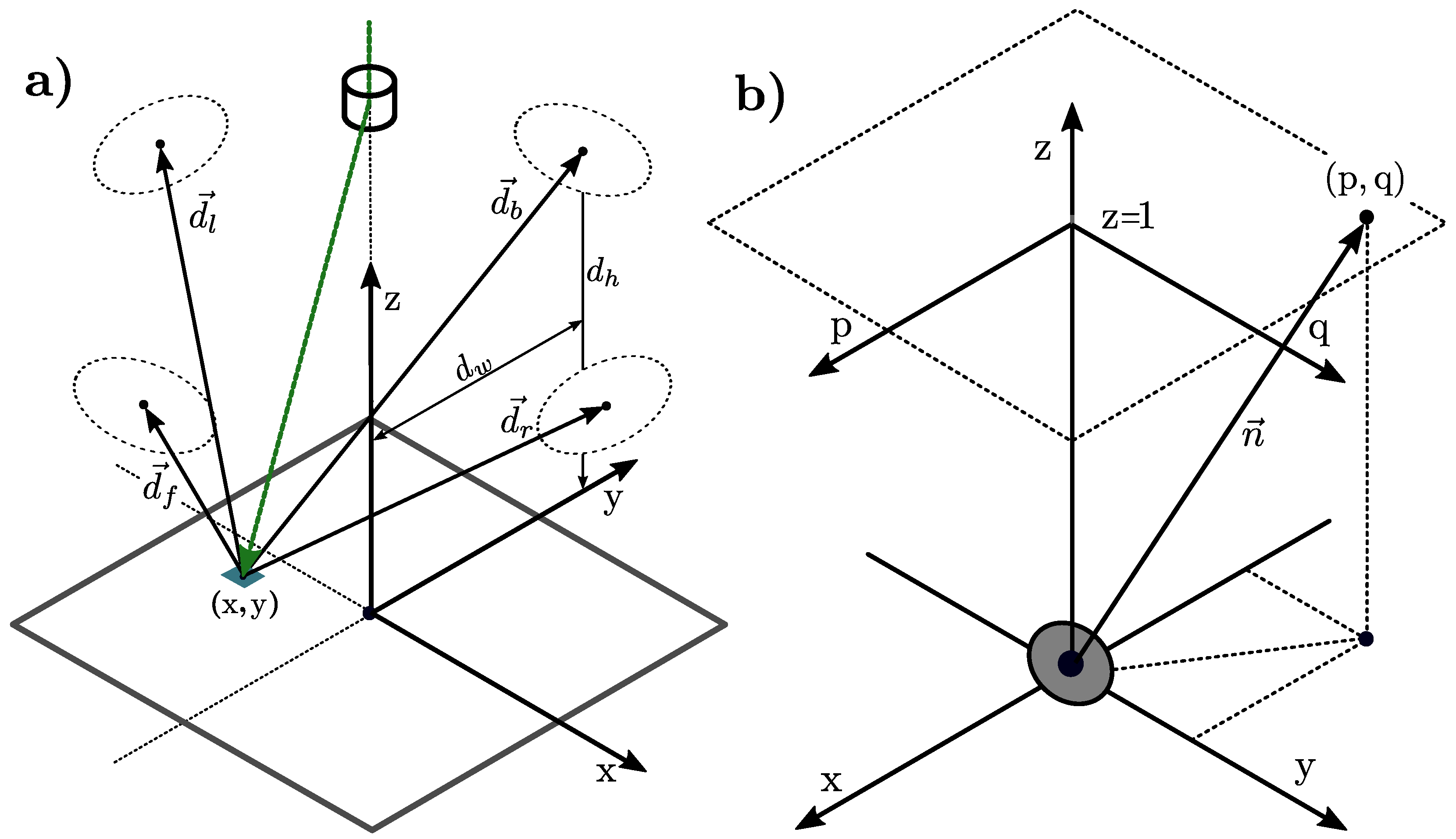
2.1.1. Model Definition

The electron beam is modelled as a single ray without any spatial extension. It hits the build surface at discrete points placed on a regular grid following the direction ${\overrightarrow{p}}_E$, as shown in Figure 1a. The build surface location $(x,y)$ is thereby approximated by the grid point $ij$, which corresponds directly to the pixel $ij$ of the later image. The beam ray stays on each grid point $ij$ for the dwell time $t_d$ and distributes

$$\begin{array}{c}\hfill N_0=\frac{I_b{t}_d}{e}\end{array}$$

(3)

PE into it, with $I_b$ describing the beam current and e the elementary charge. Then it moves instantaneously to the next grid point.

Subsequently, the PE scatter for the 1st time on the build surface at grid point location $ij$. There are $N_1$ electrons in the chamber after the 1st scattering event, which can be computed from the BSE coefficient as

$$\begin{array}{cc}\hfill N_1& =N_0\eta .\hfill \end{array}$$

(4)

More details on the computation of $\eta (E,\theta ,A)$ follow in Section 2.1.2.

For multi-detector ELO imaging, and especially the application of build surface topography reconstruction, it is reasonable to use four single detectors and align opposite detector pairs with the machine coordinate system [11]. In this work, the right and left detectors are aligned with the x-axis and the back and front detectors are aligned with the y-axis, as shown in Figure 1a. The number of electrons $N_{1,d}$ collected by a general detector d is computed by the sum of BSE, which are scattered in the detector’s solid angle ${\Omega }_d$. Equation (5) computes $N_{1,d}$ as the integral of the scattering function $g_{\mathrm{BSE}}$ over ${\Omega }_d$ as

$$\begin{array}{cc}\hfill N_{1,d}=& N_1{\int }_{{\Omega }_d}{g}_{\mathrm{BSE}}d\Omega .\hfill \end{array}$$

(5)

See Appendix A for a way to compute integrals over the solid angles of arbitrarily shaped detectors numerically. While the 1st scattering event has the biggest contribution to ELO image formation, the 2nd, 3rd, and 4th scattering events contribute additionally to the final image. In the following, the necessary equations are developed, which allow one to compute multiple scattering events on heat shields or vacuum chamber walls. See Figure 2 for a schematic of the computation of the 2nd scattering event.

The number of BSE in the vacuum chamber which can scatter a 2nd time on heat shields or the vacuum chamber walls is called $N_{1,\mathrm{Chamber}}$. Equation (6) computes $N_{1,\mathrm{Chamber}}$ as the difference of $N_1$ to the sum of all BSE which hit one of the four detectors

$$N_{1,\mathrm{Chamber}}=N_1-\sum _{d=1}^4{N}_{1,d}=N_0\eta \left(1-\sum _{d=1}^4{\int }_{{\Omega }_d}{g}_{\mathrm{BSE}}d\Omega \right).$$

(6)

As a side remark, if SE would be included at this point (in a possible model extension), then it is important to note that only BSE acts as a source for new SE from further scattering events [16]. An accurate description of this generation process needs to consider the energy distribution of BSE, which could be modelled using Monte Carlo techniques since reliable experimental data are hard to obtain [15].

To include the 2nd scattering event in the image formation, the hemisphere above grid location $ij$ is sampled uniformly with a total of l rays. These rays point in the direction ${\overrightarrow{s}}_{1,k}$, are equipped with $N_{1,k}$ electrons, and will hit the surrounding eventually. To compute $N_{1,k}$, the remaining electrons after the 1st scattering event $N_{1,\mathrm{Chamber}}$ are distributed between these rays with the help of the scattering function $g_{\mathrm{BSE}}$ as below

$$N_{1,k}=N_{1,\mathrm{Chamber}}\frac{g_{\mathrm{BSE}}({\alpha }_{1,k}, {\beta }_{1,k})}{{\sum }_{k=1}^l{g}_{\mathrm{BSE}}({\alpha }_{1,k}, {\beta }_{1,k})}.$$

(7)

The dependence of $g_{\mathrm{BSE}}$ on $d\Omega$ can be rewritten in terms of the vectors ${\overrightarrow{n}}_S$ and $\overrightarrow{d}$ and thereby in terms of the angles $\alpha$ and $\beta$ (Figure 1b), especially if the respective equations are meant to be solved numerically. More details can be found in Section 2.1.3 and Appendix A. In the case of the 2nd scattering event, ${\overrightarrow{s}}_{1,k}$ replaces $\overrightarrow{d}$ which allows to compute $N_{1,k}$ with the respective ${\alpha }_{1,k}$ and ${\beta }_{1,k}$ as defined by Equation (7). All other dependencies of $g_{\mathrm{BSE}}$ are omitted here for the sake of brevity. Naturally, none of the rays is allowed to hit a part of the detector system to avoid counting electrons scattered into the solid angles ${\Omega }_d$ multiple times. The necessary total number of rays l needs to be determined with a convergence study.

Now, the rays ${\overrightarrow{s}}_{1,k}$ replace the primary electron beam ${\overrightarrow{p}}_E$ and Equations (4) and (5) need to be solved again, but with the variables changes shown below

$$\begin{array}{cc}\hfill N_0& \to N_{1,k}\hfill \\ \hfill N_1& \to N_{2,k}\hfill \\ \hfill N_{1,d}& \to N_{2,d,k}.\hfill \end{array}$$

(8)

The total contribution of all 2nd scattering events is computed as the sum ${\sum }_k^l{N}_{2,d,k}$ which represents the total number of electrons arriving at the detector from the various scattering locations defined by the vectors ${\overrightarrow{s}}_{1,k}$.

In experiments, voltages are measured usually at the single detectors [11]. The voltage at detector d can be computed using the transimpedance T (in units of $\mathrm{V}$/$\mathrm{A}$) of a virtual amplifier in the context of the model. Therefore, Equation (9) can be used to validate simulations which include the 2nd scattering event with experimental data

$$U_d=\left(N_{1,d}+\sum _k^l{N}_{2,d,k}\right)\frac{Te}{t_d}.$$

(9)

Similarly, experimental data can be converted to a number of electrons arriving at the detector plates. The 3rd and further scattering events can be computed in the same spirit. Possible additional influences of the detector material or temperature are neglected in this work, but might be added to Equation (9). Further information on the measurement chain in ELO imaging can be found in a previous publication [11].

The above equations can be solved easily in parallel. Indeed, the algorithm can be classified as embarrassingly parallel since each grid point location is independent of the others. However, taking multiple scattering events with a high number of random rays into account demands an efficient implementation due to the exponentially growing number of calculations. It may be possible to formulate the above equations differently and more efficiently. See Reimer et al. for a comparison of electron and light optics [17] and Pharr et al. for an overview of modern ray tracing algorithms [18].

The decision to describe the electron beam with a single ray limits the models’ ability to represent resolution effects. As described above, ELO image blurring arises due to the convolution of the beam profile with the build surface, which is currently not contained in this model.

2.1.2. Back Scattered Electrons (BSE) Coefficient

The dependence of the BSE coefficient $\eta$ on E, $\theta$, and A is computed by the following phenomenological equations. Equation (10) was developed by Darlington et al. [19] for single atomic targets and was found to hold in the range of 10–100 keV

$$\eta (\theta ,A)=B{\left(\frac{{\eta }_0\left(A\right)}{B}\right)}^{cos\left(\theta \right)},\mathrm{with}B=0.89.$$

(10)

According to Reimer [16] the following expression can be used to approximate the atomic number dependence for $\theta =0$

$${\eta }_0\left(A\right)=-0.0254+0.016A-1.86\times {10}^{-4}{A}^2+8.3\times {10}^{-7}{A}^3.$$

(11)

A summary of alternative expressions for ${\eta }_0\left(A\right)$ is listed in Hermann et al. [20]; however, the differences to Equation (11) are small. Additionally, the authors provide a summary of the summing rules for multicomponent specimens and found that the following expression by Castaing [21] is the most accurate. Equation (12) allows to compute a weight averaged BSE coefficient $\overline{\eta }$, with $c_i$ being the weight fraction of the respective alloy constituent

$$\overline{\eta }=\sum _i{c}_i{\eta }_i.$$

(12)

2.1.3. Scattering Function

The scattering function $g_{\mathrm{BSE}}$ is complicated to define, especially in a numerically evaluable form. Quite a few publications exist that report experimentally measured 2D data from polar scans in polar plots [22,23], but analytical functions are scarce, especially functions which describe $g_{\mathrm{BSE}}$ fully in 3D [24]. Therefore, the classic Phong model [25] is adapted in the following way.

Equation (13) describes $g_{\mathrm{BSE}}$ by the sum of a diffusive part and a reflective part, where the latter is responsible for the experimentally found maxima of $g_{\mathrm{BSE}}$ in the forward direction at increased angles $\theta$. The arguments E and A (from Equation (1)) are dropped below for clarity. The argument $d\Omega$ is replaced by the angle $\alpha$, which is defined in Figure 1b. The reason is that Equation (5) (and similar equations computing the image contribution of further scattering events) are best solved numerically. This can be done by discretizing the detector, for example, with a triangular mesh. Now, the angle $\alpha$ points to the respective mesh element, which allows one to approximate ${\Omega }_d$ by a sum over all detector triangles; see Appendix A for more details. The diffusive part follows Lambert’s cosine law which is proportional to ∼$cos\left(\alpha \right)/\pi$, where the angle $\alpha$ is formed between the vectors ${\overrightarrow{n}}_S$ and $\overrightarrow{d}$ and $\pi$ is a normalization factor [26] as shown in Figure 1b. The reflective part forms the scattering lobe in the forward direction and is proportional to ∼${cos}^k\left(\beta \right)$

$$g_{\mathrm{BSE}}(\theta ,\alpha ,\beta )=\frac{{\eta }_0}{\pi }cos\left(\alpha \right)+\frac{\eta (\theta ,A)-{\eta }_0}{C\left(\theta \right)}\frac{k+1}{2\pi }{cos}^k\left(\beta \right).$$

(13)

The angle $\beta$ is the angle between the detection direction $\overrightarrow{d}$ and the reflection vector ${\overrightarrow{p}}_{E,\mathrm{reflected}}$ which is defined by the reflection of ${\overrightarrow{p}}_E$ on ${\overrightarrow{n}}_S$.

The parameter k describes the width of the scattering lobe and is chosen to be $k=\theta /13{}^{\circ }$ by comparison to experimental data shown in [23,24]. The diffuse part is scaled with ${\eta }_0$, whereas the reflective part is weighted with the additional electrons generated by oblique beam incidence $\eta (\theta ,A)-{\eta }_0$.

In addition, Equation (13) needs to be corrected with the function $C\left(\theta \right)$. Otherwise, the correct value of $\eta (\theta ,A)$ (from Equation (10)) at oblique electron beam incidence (or angles $\theta \gg 0$) cannot be reproduced by integrating $g_{\mathrm{BSE}}$ over the solid angle of the hemisphere ${\Omega }_{HS}$ (Equation (2)). See [27] for an analogy to rendering in light optics and why it is problematic to normalise ${cos}^k\left(\beta \right)$ analytically. The calibration function $C\left(\theta \right)$ solves this issue pragmatically. $C\left(\theta \right)$ is determined numerically by placing a hemispherical detector over the scattering location and the resulting $g_{\mathrm{BSE}}$, varying $\theta$ by changing ${\overrightarrow{n}}_S$ and measuring the number of electrons hitting the hemispherical detector. This approach is basically the numerical solution of Equation (2); again, see Appendix A for implementation details. $C\left(\theta \right)$ enforces that the phenomenological $\eta$ from Equation (10) and the numerically computed ${\eta }_n$ are equal by multiplying the reflective part with $\eta /{\eta }_n$. Equation (14) shows the calibration function $C\left(\theta \right)$, which the described procedure for Ti-6Al-4V has determined. $\theta$ is given in degree

$$C\left(\theta \right)=1.01-4.06\theta +1.36\times {10}^{-5}{\theta }^2-1.71\times {10}^{-6}{\theta }^3.$$

(14)

2.1.4. Surface Tilt and Solid Angle (STSA) Contrast Correction, Normalised Difference Images and Surface Gradient

As the introduction mentions, STSA contrast is a geometric effect resulting from detector positioning and size. It needs to be corrected to enable various applications in ELO imaging, here, the focus is on surface topography reconstruction. Surface tilt contrast develops due to the dependence of $\eta$ on $\theta$ as defined in Equation (10). In the most simple case, the angle $\theta$ is equal to the deflection angle $\varphi$ which means that the local surface normal vector ${\overrightarrow{n}}_S={[0,0,1]}^T$ and, therefore, ${\overrightarrow{n}}_S$ is parallel to the z-axis. Both angles depend on the build surface location $(x,y)$ and increase with distance to the machine coordinate system centre. Consequently, $\eta$ decreases. Solid angle contrast is a result of the dependence of Equation (5) on the build surface location $(x,y)$. Both, ${\Omega }_d$ and $g_{\mathrm{BSE}}$ vary with $(x,y)$ and, therefore, the integral varies. Naturally, the same holds true if multiple scattering events are included (as indicated by Equation (9)), but then the respective vacuum chamber interior location replaces the build surface location.

The basis for the computation of the build surface gradient $\nabla \overline{Z}(x,y)$ are STSA contrast corrected normalised difference images. ELO images for STSA contrast correction can be recorded from a plane plate characterised by ${\overrightarrow{n}}_S\approx {[0,0,1]}^T$. Then single ELO images of the right, left, back, and front detectors are normalised with the correction images to obtain the contrast-corrected images $R^C$, $L^C$, $B^C$, and $F^C$. The corrected normalised difference image $M_x$ and $M_y$ are computed by the respective expression below

$$\begin{array}{c}\hfill M_x=\frac{R^C-L^C}{R^C+L^C}\mathrm{and}{M}_y=\frac{B^C-F^C}{B^C+F^C}.\end{array}$$

(15)

$M_x$ carries gradient information along the x-axis whereas $M_y$ carries gradient information along the y-axis. The gradient $\nabla \overline{Z}(x,y)$ is then obtained from $M_x$ and $M_y$ after further computation and calibration steps. In addition to STSA contrast, normalised difference images do not depend on the beam current $I_B$ and on the backscattering coefficient $\eta$, as described in detail in [11].

Following the arguments in [28,29] shows that the projection model of the imaging process defines the connection of local surface normal vector ${\overrightarrow{n}}_S$ at location $(x,y)$ and $\nabla Z(x,y)$. The ELO projection model defined in [11] reveals that ELO imaging does not exactly follow orthographic projection, but it is a valid simplification as long as the work distance $w_d$ (Figure 1a) is big in comparison to the build surface height $Z(x,y)$. Then ${\overrightarrow{n}}_S$ can be written in terms of the gradient as

$${\overrightarrow{n}}_S=\left[\begin{array}{c}-\frac{\partial Z}{\partial x}\\ -\frac{\partial Z}{\partial y}\\ 1\end{array}\right]=\left[\begin{array}{c}{n}_{Sx}\\ n_{Sy}\\ 1\end{array}\right].$$

(16)

Summarizing, this means that multi-detector ELO imaging enables the measurement of the normal vector field of the build surface, which can be reconstructed using existing normal integration algorithms.

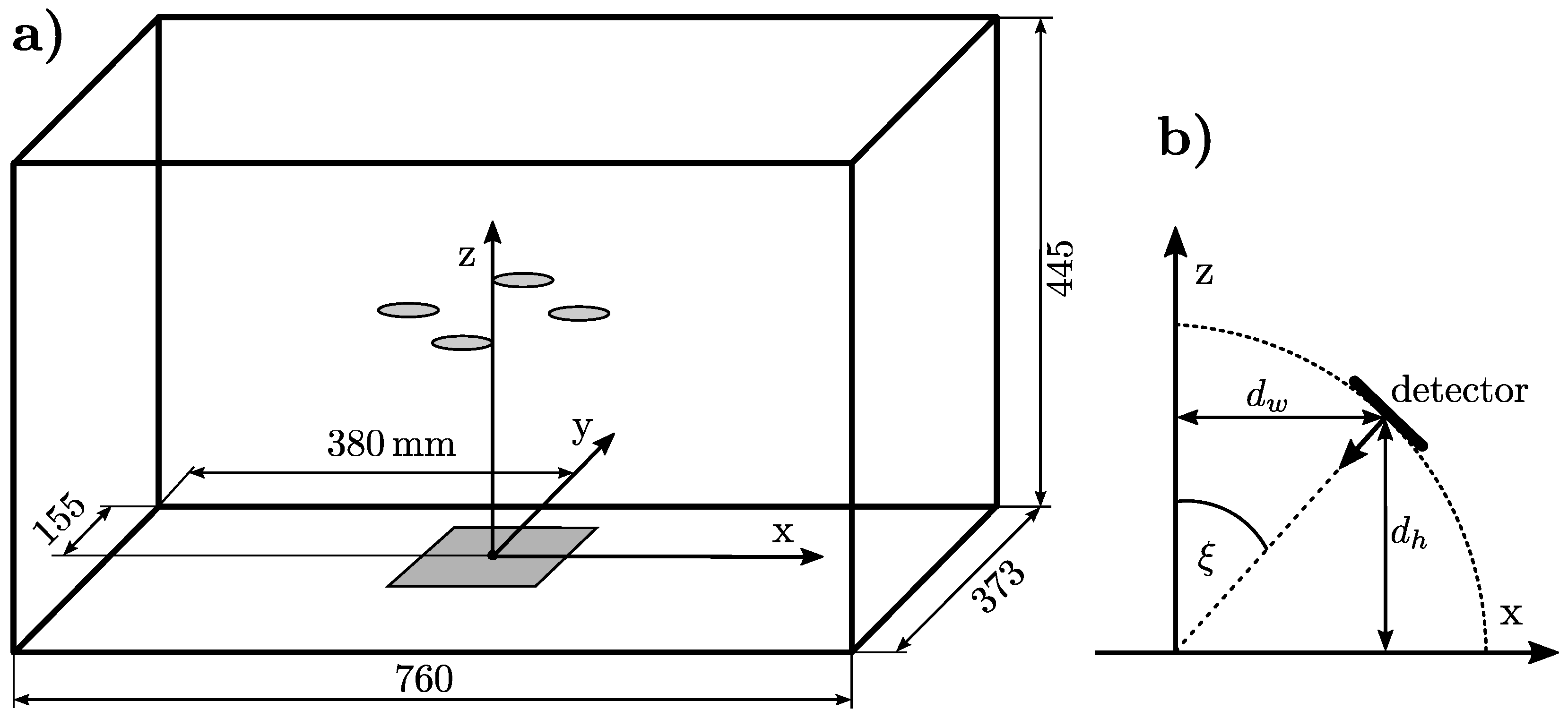
2.2. Validation Experiments

The validation experiment was conducted on the in-house developed PBF-EB system ATHENE and reported on in detail in a previous publication [11]. In brief, the experiment consists of the recording of ELO images of a blank Ti-6Al-4V melt plate for STSA contrast correction, melting of 3 × 3 squares with a side length of 10 $\mathrm{m}$$\mathrm{m}$ and 15 $\mathrm{m}$$\mathrm{m}$ on the same plate and the subsequent recording of further ELO images. The Ti-6Al-4V melt plate in Figure 3a is the result and is used to validate simulation results of the presented ray tracing model. Figure 3b shows the height map $Z(x,y)$ of the melt plate, which was measured with the optical profilometer Keyence VR-6200.

The acceleration voltage of the electron beam gun is 60 $\mathrm{k}$$\mathrm{V}$. The exact melt parameters are given in [11] since they are of no further importance in this work.

All ELO images were recorded with a four-detector system under a controlled vacuum atmosphere of $1.5\times {10}^{-3}$ mbar generated by a constant helium influx. A beam current of 3 $\mathrm{m}$$\mathrm{A}$ was chosen at a scan speed of $v_S=133 \mathrm{m}{\mathrm{s}}^{-1}$. The side length of the images was 80 $\mathrm{m}$$\mathrm{m}$ with 1500 single scan lines, which results in a square pixel size of $53.3$ $\mathsf{\mu }$$\mathrm{m}$ and a dwell time of $t_d=0.4 \mathsf{\mu }\mathrm{s}$.

The detectors are placed at a height of $d_h=272 \mathrm{m}\mathrm{m}$ and spaced $d_w=127 \mathrm{m}\mathrm{m}$ from the z-axis of the machine coordinate system (as depicted schematically in Figure 1a). The normal vectors of all four detectors are directed towards the centre of the coordinate system, as shown in Figure 5b. The right and left detectors are aligned with the x-axis and record the images R and L, whereas the back and front detectors are aligned with the y-axis and record B and F. The single detector disks are made from copper with a diameter of 50 $\mathrm{m}$$\mathrm{m}$. Heat shields are omitted deliberately from the experiment. More details on the measurement chain and the choice of cabling used amplifiers and digitisers can be found in [11].

2.3. Software

The ELO raytracing model is implemented using open-source libraries of the scientific Python community. In principle, an ELO imaging experiment can be recreated virtually by designing a digital twin of the experimental setup. NumPy [30] and Scipy [31] are used as a basis. For example, the Ti-6Al-4V plate in Figure 3a is digitised from the height map $Z(x,y)$ in Figure 3b by creating a mesh with the library Open3D [32] and exported as .stl file. All further surfaces in the simulation, a flat plate for STSA contrast correction, the detector plates, and the vacuum chamber of the PBF-EB machine are drawn with a CAD program and then exported as single .stl files. The library trimesh [33] is used to load the .stl files and to represent the simulation environment in the form of meshes. Additionally, trimesh computes the intersection of single rays with the respective meshes. Scikit-image [34] is used for all image processing tasks, and Matplotlib [35] and CMasher [36] for plotting.

2.4. Simulations

The following simulation parameters are kept constant throughout this work. The acceleration voltage is 60 $\mathrm{k}$$\mathrm{V}$, the beam current is 3 $\mathrm{m}$$\mathrm{A}$, the dwell time $t_d=0.4 \mathsf{\mu }\mathrm{s}$ and the transimpedance $T=1 \times {10}^5\mathrm{V}/\mathrm{A}$. Further, only BSE contributes to the detector signals, following the arguments presented in Appendix B. Only the 1st scattering event is computed in the model, except stated otherwise. All objects of interest consist of Ti-6Al-4V; this means that Equation (10) is computed as a weighted sum using Equation (12). The specific detector positioning of the various simulation studies is mentioned where necessary.

Validation

The validation simulations mirror the detector system positioning of the validation experiment described in Section 2.2. To validate STSA contrast, a plane plate (characterised by ${\overrightarrow{n}}_S={[0,0,1]}^T$) is used as an object of interest. Here the 1st and additionally the 2nd scattering event are computed to account for the influence of the vacuum chamber interior. The digitised Ti-6Al-4V melt plate is used to validate STSA-corrected normalised difference images $M_x$ and $M_y$ since they are the basis for gradient computation. The simulated ELO images R, L, B, and F are divided by the respective STSA images to obtain the STSA corrected images $R^C$, $L^C$, $B^C$, and $F^C$. Then $M_x$ and $M_y$ are computed using Equation (15). The experimentally recorded $M_x$ and $M_y$ are computed analogously.

3. Results

This part is concerned with validating the ELO ray tracing model by comparing experimental and modelled STSA contrast ELO images. Additionally, STSA contrast corrected normalised difference images $M_x$ of the Ti-6Al-4V melt plate displayed in Figure 3 are computed from experimental and modelled ELO images and compared.

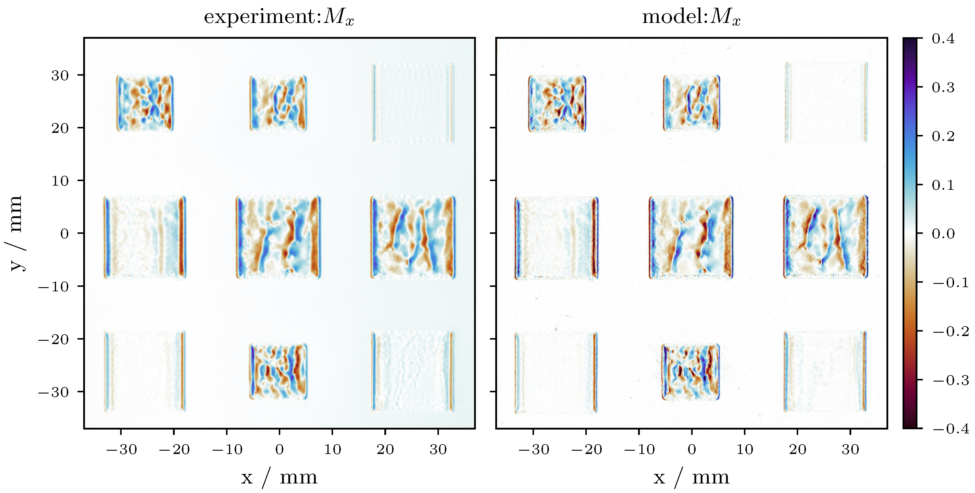
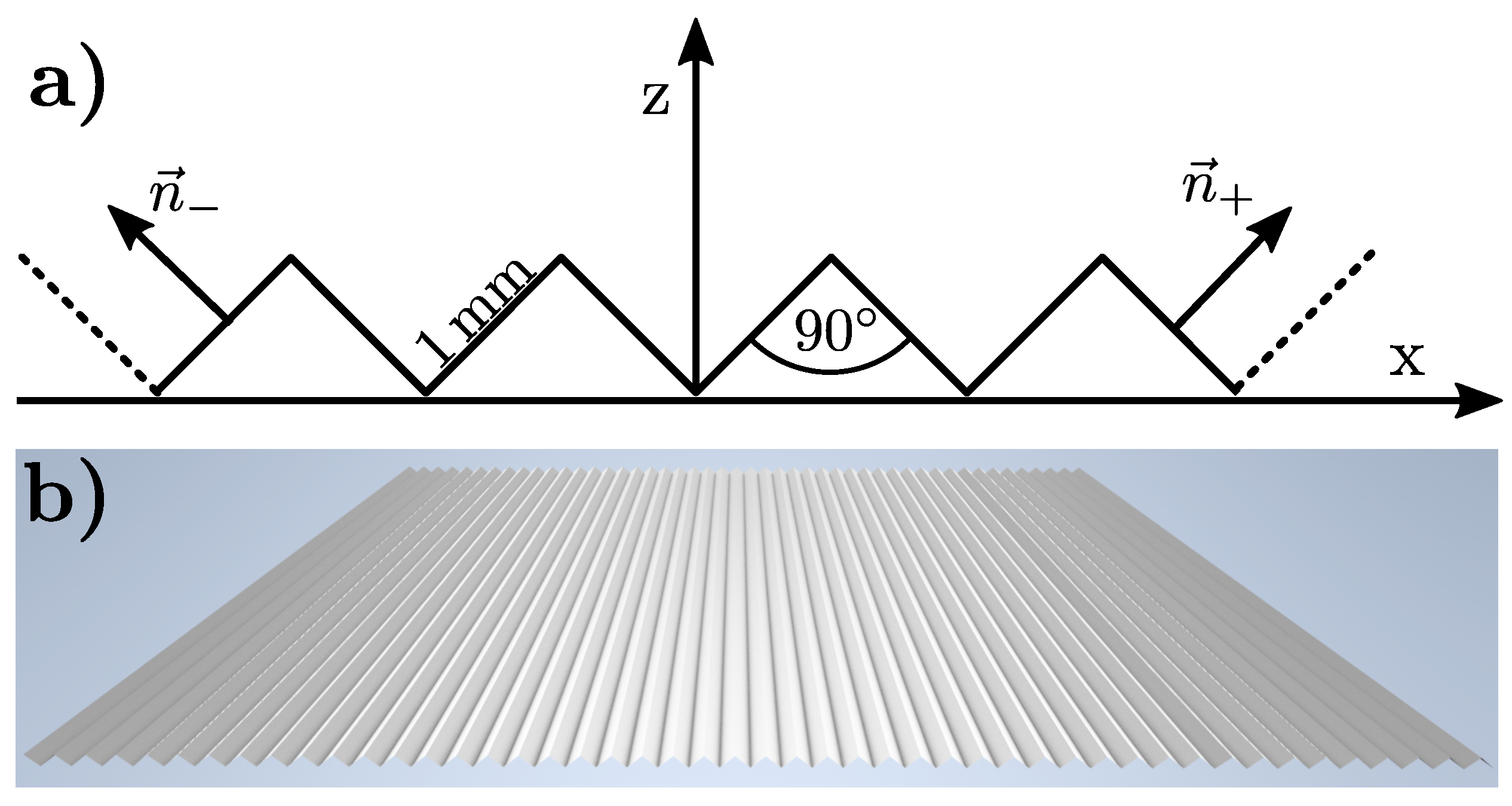
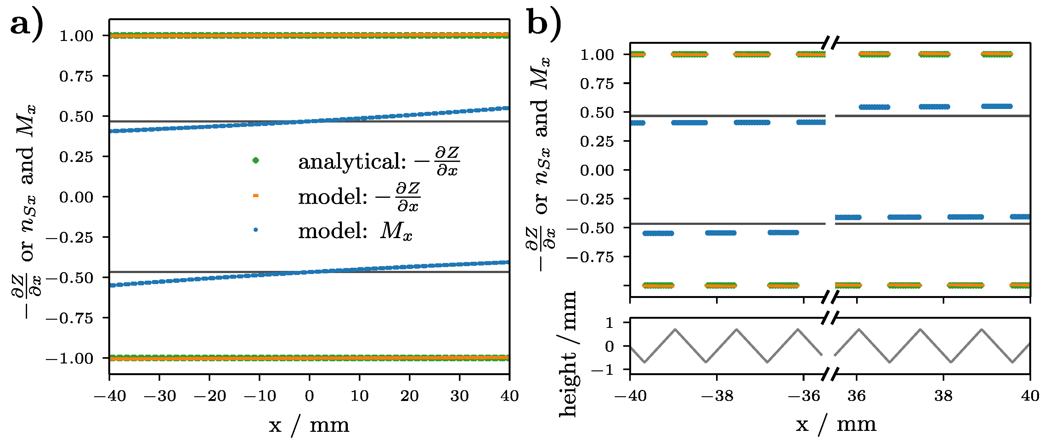
3.1. Validation: STSA Contrast

As explained in the introduction, STSA contrast correction is a necessary step to compute surface gradients. Therefore, the first part of the validation study compares STSA images of the validation experiment and the model in Figure 4, as recorded by the right detector. The object of interest is a blank plate Ti-6Al-4V plate characterised by a local normal surface vector ${\overrightarrow{n}}_s={[0,0,1]}^T$. All images display the quotient of input electrons arriving at the detector by normalizing with $N_0$. As a rule of thumb, roughly one-thousandth of the input electrons arrive at the detectors in this specific setting. The current arriving at the detectors is in the range of $\mathsf{\mu }\mathrm{A}$ range since the input current $I_B=3\mathrm{m}\mathrm{A}$.

The curvature of the contour lines of the experimentally recorded ELO image in Figure 4a are parabolic however, there is an asymmetry at the upper end. In contrast, the simulated ELO image of the 1st event in Figure 4b is symmetric with respect to the x-axis. Including the 2nd event in the calculation means that the influence of the vacuum chamber interior is added to the image formation. Figure 4d shows the 2nd scattering event isolated, and clearly, there is no recognizable symmetry. Adding the contribution of the 1st and 2nd scattering events reproduces the contour line asymmetry as shown in Figure 4d.

The asymmetric image contribution of the 2nd scattering event can be explained by the specific vacuum chamber interior of ATHENE. As shown schematically in Figure 5a, the machine coordinate system is placed closer to the back side (since a radiation protection metal sheet hangs from the ceiling) than to the front side. The detector’s solid angle from a position on the back side will, therefore, be always bigger than the detector’s solid angle from a comparable position on the front side. Consequently, more electrons reach the right detector from the back side.

This result is quite significant for future optimised multi-detector systems. Clearly, the vacuum chamber interior, for example, heat shields, will distort ELO images due to the 2nd and further scattering events. Therefore, future heat shields should be symmetric with respect to the z-axis of the machine coordinate system and the scan pattern or even be designed to minimise the influence of every scattering event after the 1st.

While the degree of similarity between the experiment and model is astonishing the model overestimates the experiment slightly on a quantitative level. This can be explained by the assumptions of the ELO ray tracing model, as described in Section 2.1. Possible extensions of the model can either increase or decrease the intensities of the modelled images. Including backscattering on the detector plates itself or accounting for the influence of helium gas will decrease the number of electrons arriving at the detectors. However, including further scattering events (besides the 1st and 2nd), adding the signal contribution of SE, or using a more accurate, experimentally verified definition of $g_{\mathrm{BSE}}$ might increase the number of electrons arriving at the detectors.

Further, the detector material itself and inaccuracies in detector positioning are suspected to influence the experiments and could be responsible for the difference in the model.

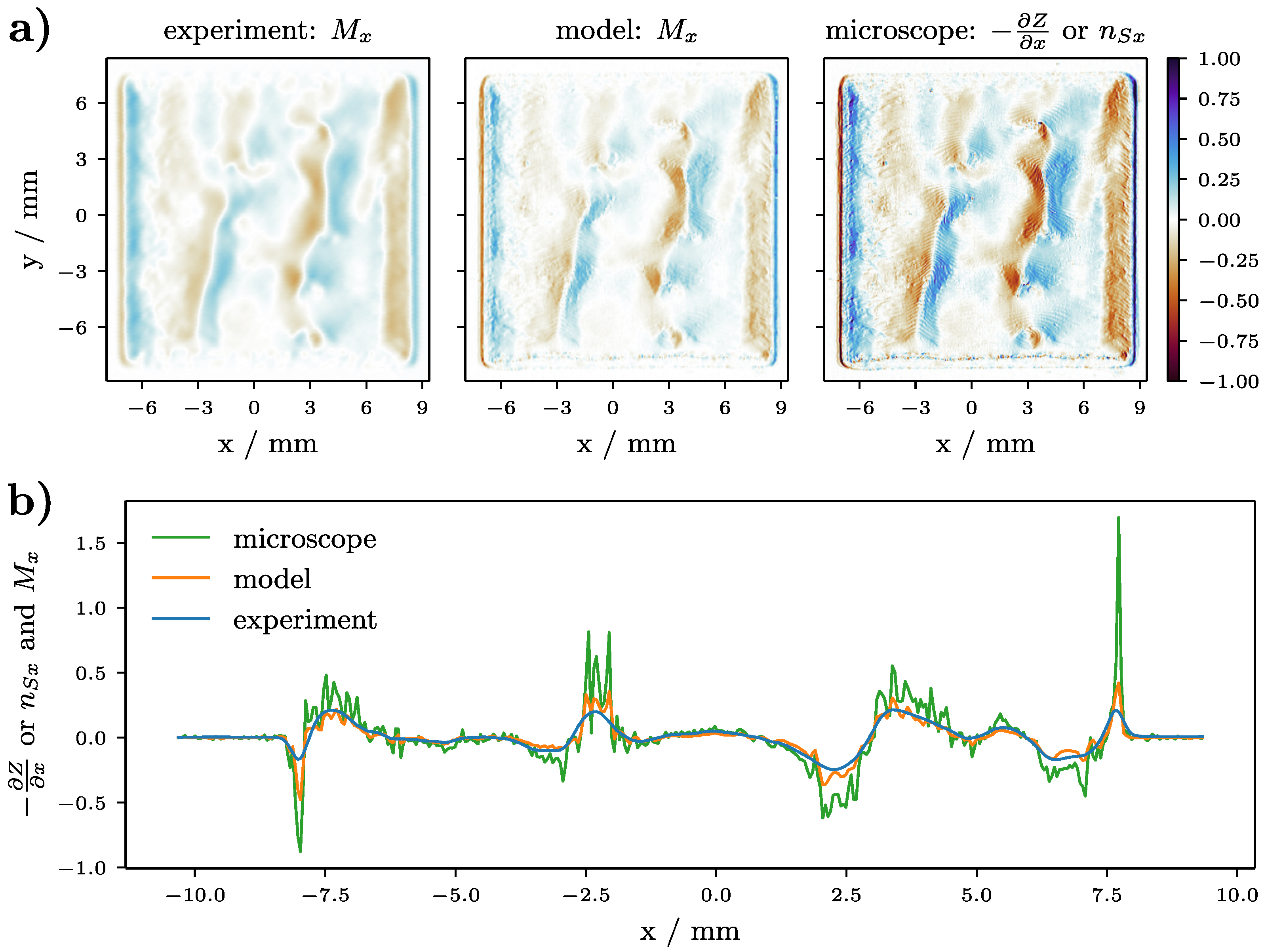
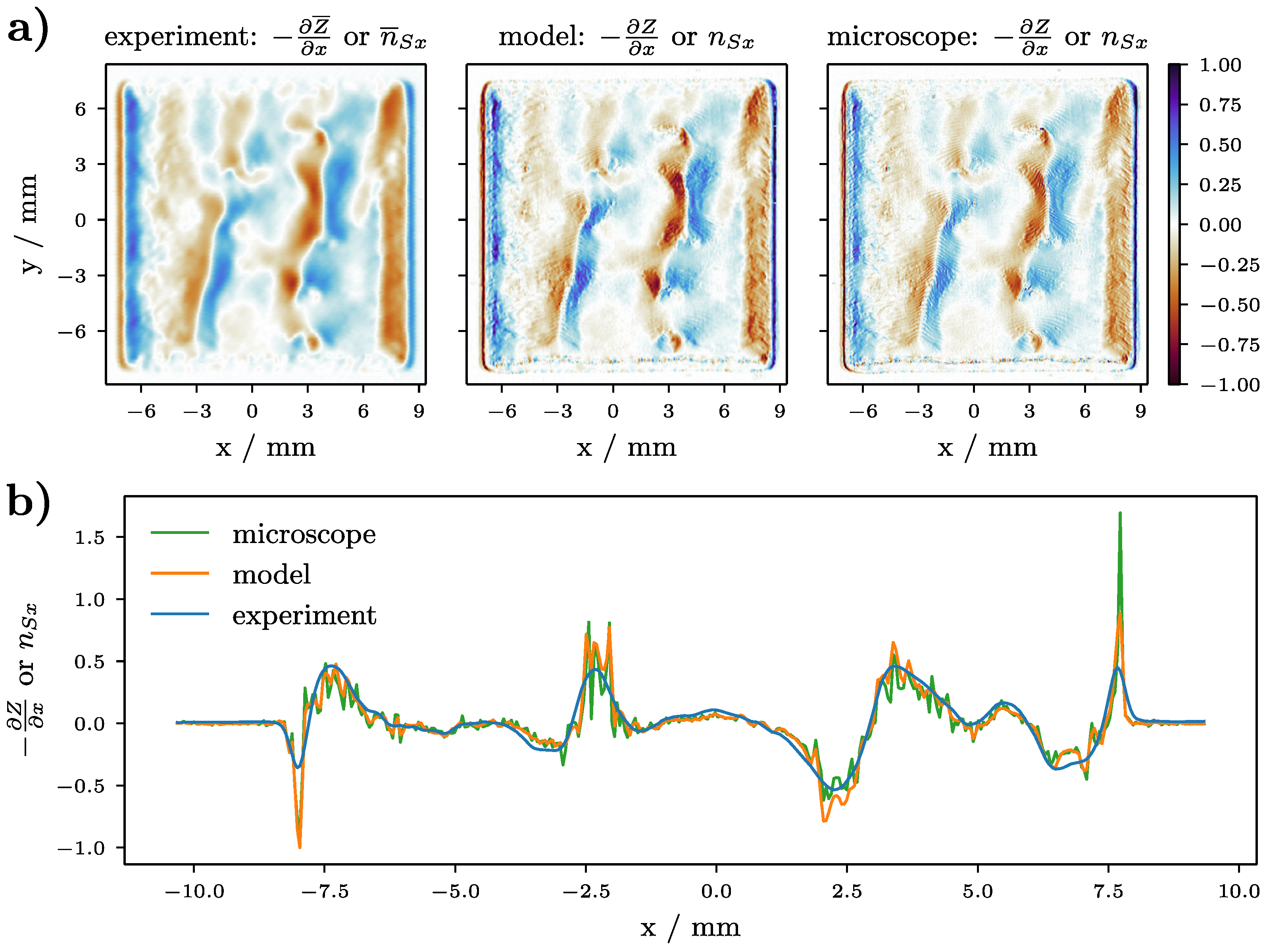
3.2. Validation: Melt Plate

Figure 6 compares the experimentally recorded STSA contrast corrected normalised difference image $M_x$ with the computed one. As explained in Section 2.1.4, the material contrast information, the influence of the beam current $I_b$ and STSA contrast are removed from $M_x$ (and $M_y$). This explains the astonishing similarity between the experiment and the model. A deviation of $M_x$ from the expected value of zero can be observed aside the melt surfaces (characterised by ${\overrightarrow{n}}_S$ parallel to the z-axis), which can be explained by slight misalignments of detector plates, the melt plate or calibration issues of the measurement chain [11].

Figure 7 compares $M_x$ of the experiment and model with the true gradient $\partial Z/\partial x$ (obtained from the height map in Figure 3b) at the example of the middle surface of the Ti-6Al-4V melt plate. The experimental $M_x$ in Figure 7a appears blurred in comparison to the model, which can be explained by the effect of the beam profile. The beam profile on ATHENE is approximately Gaussian in the focus point at the machine coordinate system centre and shows a beam diameter of approximately 270 $\mathsf{\mu }$$\mathrm{m}$ full-width half maximum. Even though many of the fine details vanish, both images are quite similar. However, the comparison with the true gradient $\partial Z/\partial x$ reveals immediately that $M_x$ of the model and experiment do not reach the magnitude of the true gradients. Figure 7b compares profile plots along x at $y=0$ of the three images above, naturally with the same conclusion.

The effect has been noticed in previous work and could be corrected by scaling normalised difference images with calibration functions obtained from ELO images of a calibration object with known dimensioning [11]. However, the root cause for the magnitude difference remained unknown. An additional close look at the model and microscope measurement shows that the digitization of the height map (via mesh generation) has a slight averaging effect but without significant influence.

4. Discussion

The following part identifies the root cause of the magnitude differences of $M_x$ and $M_y$ to the true gradient $\nabla Z(x,y)$ with the help of a simplified model of ELO image formation. An equation to compute an experimentally measured $\nabla \overline{Z}(x,y)$ directly from four ELO images recorded by a suitable detector system is developed. The equation is tested with the accurate ELO ray tracing model on the corrugated sheet of Section 4.2 and further validated with experimentally recorded ELO images of the Ti-6Al-4V melt plate. Additionally, detector positioning and its influence on masking and contrast development in ELO image formation are discussed.

4.1. Distortion Effects in Gradient Computation

In the following, the complex model of Section 2.1 is simplified twofold. First, the areal detector is shrunk to a point-like detector and second the scattering function $g_{\mathrm{BSE}}$ is assumed to be simply Lambert’s cosine law. This allows approximating Equation (5) by the vector definition of the cosine function. In consequence the influence of the geometric parameters of the detector system $d_w$ and $d_h$ is made explicit by the following detector vector definition.

The detector vectors ${\overrightarrow{d}}_r,{\overrightarrow{d}}_l,{\overrightarrow{d}}_b$ and ${\overrightarrow{d}}_f$ (of the right, left, back, and front detector) are defined at the surface plane point $(x,y)$ as

$${\overrightarrow{d}}_r=\left[\begin{array}{c}\frac{d_w-x}{d_h}\\ \frac{-y}{d_h}\\ 1\end{array}\right],{\overrightarrow{d}}_l=\left[\begin{array}{c}\frac{-d_w-x}{d_h}\\ \frac{-y}{d_h}\\ 1\end{array}\right]\mathrm{and}{\overrightarrow{d}}_b=\left[\begin{array}{c}\frac{-x}{d_h}\\ \frac{d_w-y}{d_h}\\ 1\end{array}\right],{\overrightarrow{d}}_f=\left[\begin{array}{c}\frac{-x}{d_h}\\ \frac{-d_w-y}{d_h}\\ 1\end{array}\right].$$

(17)

Figure 8a illustrates the simplified multi-(point)-detector system and the $x,y$-position dependency of the detector vectors.

Additionally, the local surface normal vector ${\overrightarrow{n}}_S$ and the surface vector of the STSA contrast correction plate ${\overrightarrow{n}}_C$ are defined by

$${\overrightarrow{n}}_S=\left[\begin{array}{c}{n}_{Sx}\\ n_{Sy}\\ 1\end{array}\right]\mathrm{and}{\overrightarrow{n}}_C=\left[\begin{array}{c}0\\ 0\\ 1\end{array}\right].$$

(18)

The z-component of every vector is normalised to 1 by scaling every vector until it touches the plane $z=1$, as shown schematically by Figure 8b. Usually, this representation is called $p,q$-form. It is chosen here intentionally since a four-detector system composed of orthogonal detector pairs can only measure two components of a given 3D normal vector ${\overrightarrow{n}}_S$, but not all three.

In the following, the images $R,L,B$ and F are computed by the respective Equation (19) as functions of the build surface position $(x,y)$. Every detector vector and surface vector changes with a given $(x,y)$ and so does $\eta$, but this and all other dependencies are omitted in the following for the sake of brevity

$$\begin{array}{cc}\hfill R=& \frac{N_0\eta }{\pi }\frac{{\overrightarrow{n}}_S·{\overrightarrow{d}}_r}{\left|{\overrightarrow{n}}_S\right|\left|{\overrightarrow{d}}_r\right|}\mathrm{and}L=\frac{N_0\eta }{\pi }\frac{{\overrightarrow{n}}_S·{\overrightarrow{d}}_l}{\left|{\overrightarrow{n}}_S\right|\left|{\overrightarrow{d}}_l\right|}\hfill \\ \hfill B=& \frac{N_0\eta }{\pi }\frac{{\overrightarrow{n}}_S·{\overrightarrow{d}}_b}{\left|{\overrightarrow{n}}_S\right|\left|{\overrightarrow{d}}_b\right|}\mathrm{and}F=\frac{N_0\eta }{\pi }\frac{{\overrightarrow{n}}_S·{\overrightarrow{d}}_f}{\left|{\overrightarrow{n}}_S\right|\left|{\overrightarrow{d}}_f\right|}.\hfill \end{array}$$

(19)

The STSA correction image C of an arbitrary detector is then simply given by

$$C=\frac{N_0{\eta }_C}{\pi }\frac{1}{|\overrightarrow{d}|},$$

(20)

where ${\eta }_C$ is the BSE coefficient of a plane plate defined by ${\overrightarrow{n}}_C$. This allows to compute the respective STSA corrected images by $R/C_R,L/C_L,B/C_B$ and $F/C_F$ as

$$\begin{array}{cc}\hfill R^C=& \frac{\eta }{{\eta }_C}\frac{{\overrightarrow{n}}_S·{\overrightarrow{d}}_r}{|{\overrightarrow{n}}_S|}\mathrm{and}{L}^C=\frac{\eta }{{\eta }_C}\frac{{\overrightarrow{n}}_S·{\overrightarrow{d}}_l}{|{\overrightarrow{n}}_S|}\hfill \\ \hfill B^C=& \frac{\eta }{{\eta }_C}\frac{{\overrightarrow{n}}_S·{\overrightarrow{d}}_b}{|{\overrightarrow{n}}_S|}\mathrm{and}{F}^C=\frac{\eta }{{\eta }_C}\frac{{\overrightarrow{n}}_S·{\overrightarrow{d}}_f}{|{\overrightarrow{n}}_S|}.\hfill \end{array}$$

(21)

Consequently, this means that STSA contrast correction removes the imaging current dependency in form of $N_0$ and the normalization constant $\pi$. Additionally, the norm of the respective detector vector is removed. This last point is equivalent to the solid angle dependency in experiments or the ELO ray tracing model. Inserting the detector vector definitions in the scalar products allows writing the STSA-corrected difference images as

$$\begin{array}{cc}\hfill R^C-L^C=& \frac{\eta }{{\eta }_C}\frac{2}{|{\overrightarrow{n}}_S|}\frac{n_{Sx}{d}_w}{d_h}\hfill \\ \hfill B^C-F^C=& \frac{\eta }{{\eta }_C}\frac{2}{|{\overrightarrow{n}}_S|}\frac{n_{Sy}{d}_w}{d_h}.\hfill \end{array}$$

(22)

Equation (22) shows that the difference image $R^C-L^C$ measures the x component of ${\overrightarrow{n}}_S$ scaled by the detector position given by $d_w$ and $d_h$. Equivalently, $B^C-F^C$ measures the y component of ${\overrightarrow{n}}_S$. Additionally, the vector component information is divided by $|{\overrightarrow{n}}_S|$ and the quotient of the scattering coefficients. The STSA corrected sum images are given by

$$\begin{array}{c}\hfill R^C+L^C=\frac{\eta }{{\eta }_C}\frac{2}{|{\overrightarrow{n}}_S|}\left[1-\frac{n_{Sx}x+n_{Sy}y}{d_h}\right]=B^C+F^C.\end{array}$$

(23)

The sum images are intended to measure only the local material contrast without surface topography influence. However, the scattering coefficient $\eta$ contains a dependence on the angle $\theta$ and thereby on ${\overrightarrow{n}}_s$, as shown by Equation (10) and Figure 1b. Additionally, the sum images are superimposed with $1/|{\overrightarrow{n}}_S|$ and distorted by the term $(n_{Sx}x+n_{Sy}y)/d_h$. This is an important result for optimised multi-detector designs since the undesired effects can be partly suppressed simply by increasing the detector distance $d_h$. Further, accurate knowledge of ${\overrightarrow{n}}_S$ might allow to correct Equation (23) for all remaining influences of topography.

The normalised difference images are computed by dividing Equations (22) by Equation (23) to obtain

$$\begin{array}{cc}\hfill M_x=\frac{R^C-L^C}{R^C+L^C}=& \frac{n_{Sx}{d}_w}{d_h-(n_{Sx}x+n_{Sy}y)}\hfill \\ \hfill M_y=\frac{B^C-F^C}{B^C+F^C}=& \frac{n_{Sy}{d}_w}{d_h-(n_{Sx}x+n_{Sy}y)}.\hfill \end{array}$$

(24)

This formulation explains the magnitude difference of $M_x$ (and $M_y$) to $\nabla Z(x,y)$ depicted in Figure 7 directly. Obviously the respective ${\overrightarrow{n}}_S$ component and thereby $\nabla Z(x,y)$ is scaled in first approximation with $d_w/d_h$. Additionally, the expressions confirm that the material contrast information disappears completely (as intended), but as a drawback, the division with the sum images adds the known position-dependent distortion. A careful look shows that a given vector ${\overrightarrow{n}}_{+}={[1,0,1]}^T$ is measured as $d_w/d_h$ at $x=0$, whereas it is measured as $d_w/(d_h\pm x)$ depending if $x<0$ or $x>0$. Naturally, the same holds for a general ${\overrightarrow{n}}_S$. The distortion is a deeply unsatisfying consequence of the STSA contrast correction and thereby of the non-linearity of the scattering function, in this case of Lambert’s cosine law.

The distortion effect can be corrected by rearranging Equations (24) and solving for the only two unknowns, $n_{Sx}$ and $n_{Sy}$ to obtain

$$n_{Sx}=\frac{M_x(d_h-n_{Sy}y)}{d_w+x{M}_x}\mathrm{and}{n}_{Sy}=\frac{M_y(d_h-n_{Sx}x)}{d_w+y{M}_y}.$$

(25)

It is possible to solve for the normal vector components of ${\overrightarrow{n}}_S$ by inserting the respective Equation (25) into the other. In summary, Equation (26) computes $\nabla Z(x,y)$ directly from the normalised differences images $M_x$ and $M_y$ and the detector position as

$$-\frac{\partial Z}{\partial x}=n_{Sx}=\frac{M_x{d}_h}{d_w+x{M}_x+y{M}_y}\mathrm{and}-\frac{\partial Z}{\partial y}=n_{Sy}=\frac{M_y{d}_h}{d_w+x{M}_x+y{M}_y}.$$

(26)

4.2. Correct Gradient Computation

The corrugated sheet object depicted in Figure 9 is used to test if the predictions by Equations (24) and (26) are valid in the framework of the ELO ray tracing model. The object is characterised by neighbouring flanks of 1 $\mathrm{m}$$\mathrm{m}$ length with surface normals ${\overrightarrow{n}}_{-}={[-1,0,1]}^T$ and ${\overrightarrow{n}}_{+}={[1,0,1]}^T$. The resulting pattern extends along the x-axis but does not change along y, which allows us to isolate position-dependent distortion effects. $M_x$ and $M_y$ are obtained from modelled ELO images. The detectors are placed at a height of $d_h=272 \mathrm{m}\mathrm{m}$ and single detectors are $d_w=127 \mathrm{m}\mathrm{m}$ away from the z-axis of the machine coordinate system, as in the validation study.

Figure 10 compares line profiles along x at $y=0$ of $M_x$ with the true, analytical gradient $\partial Z/\partial x$ and the computed $\partial Z/\partial x$ from ELO images. $M_x$ is always lower than the true analytical gradients, as could be expected by the results from Section 3.1 and Equation (24). At $x=0$, $M_x$ takes the value $d_w/dh\approx 0.47$. Additionally, $M_x$ shows a build area position dependency which is predicted from Equation (24). The analytical gradient $\partial Z/\partial x$ equals $\pm 1$ depending on the rising or falling flank of the object. The modelled gradient $\partial Z/\partial x$ follows the analytical one to a very high degree, which confirms the correctness of Equation (26) in the framework of the ELO ray tracing model.

Figure 11 displays the middle surface of the Ti-6Al-4V melt plate as in Section 3.1. However, now the experimental and the modelled gradients are computed from the respective Equation (26) and compared to the gradient computed from the microscope measurement. Figure 11a reveals that the order of magnitude of the experimental $\partial \overline{Z}/\partial x$ matches with $\partial Z/\partial x$ obtained from model and microscope measurement. Differences between the experiment, model, and microscope measurement can be explained again by the influence of the beam profile on the ELO image formation. Figure 11b shows that the line profiles along x at $y=0$ match closely. Differences between the gradient of the model and microscope measurement are attributed to the digitization of the height map.

This part establishes that STSA contrast corrected normalised difference images $M_x$ and $M_y$ depend on the recording position $(x,y)$. The unintended positional dependence can be completely removed by Equations (26), which allow computing $\nabla \overline{Z}(x,y)$ directly from experimentally recorded ELO images without the need of any additional calibration functions. Knowledge of the constructive details of the detector system, the detectors heights $d_w$, and their distance from the z-axis $d_w$ are enough to directly compute the surface gradient $\nabla \overline{Z}(x,y)$ from the four ELO images of a multi-detector system. To the author’s knowledge, this is valid for the simplified point-detector model, the ELO Raytracing model, and the true scattering function of the validation experiments. This is a big improvement to the surface topography reconstruction algorithm presented in a previous publication [11] and its future applicability.

4.3. Scattering Function, Detector Positioning and Masking

In rendering and photometric stereo, reflectance maps establish a clear visual relation between image brightness at a given surface orientation when the light source direction and surface reflectance are known [29,37]. This study is concerned with electron optics, however, the concept of reflectance maps can be applied as well [17].

As described in Section 2.1 (and Appendix A), the pixel intensity of ELO images develop due to the interplay of scattering function, detector position $\overrightarrow{d}$ (or solid angle) and the local surface normal vector ${\overrightarrow{n}}_S$. Assuming a point-like detector and vertical electron beam incidence (${\overrightarrow{p}}_E={[0,0,-1]}^T$) and further positioning every local ${\overrightarrow{n}}_S$ at the coordinate system centre allows to compute a reflectance map for the 1st scattering event. To this end, the vectors $\overrightarrow{d}$ and ${\overrightarrow{n}}_S$ are defined in $p,q$- form, as illustrated in Figure 8b and explained in Section 4.1. Every cartesian vector $\overrightarrow{n}={[n_x,n_y,n_z]}^T$ is scaled such that it touches the $p,q$- plane defined at the height $z=1$ and consequently $n_z=1$. The reflectance maps can then be computed by evaluating Equation (13) with a given $\overrightarrow{d}$ and ${\overrightarrow{n}}_S$ and displayed by plotting the result at the respective position $(n_{Sx},n_{Sy})$ in 2D.

Figure 12 and Figure 13 show the reflectance maps of two different positions of a right detector ${\overrightarrow{d}}_r={[d_w/d_h,0,1]}^T$ (indicated by white crosses) resulting in detector inclinations of $\xi =25{}^{\circ }$ and $\xi =50{}^{\circ }$ (see Figure 1a and Figure 5b.). The left side of both figures displays the reflectance map due to the complete scattering function $g_{\mathrm{BSE}}$ whereas the right side shows only the reflectance map due to the diffusive part. Both figures display hatched areas that indicate masked vectors ${\overrightarrow{n}}_S$. In this specific geometric condition, the right detector is placed along the p-axis (or x-axis). The masking condition for any ${\overrightarrow{n}}_S$ is, therefore, given by $n_{Sx}\le -d_h/d_w$, irrespective of $n_{Sy}$. This means that the detector vector ${\overrightarrow{d}}_r$ and ${\overrightarrow{n}}_S$ enclose an angle $\alpha \ge |\pi /2|$ and subsequently $g_{\mathrm{BSE}}(\theta ,\alpha ,\beta )=0$ since electrons cannot reach the detector directly and the ELO pixel intensity is zero. In general, every surface vector ${\overrightarrow{n}}_S={[n_{Sx},n_{Sy},1]}^T$ imaged with a detector at $\overrightarrow{d}={[d_x,d_y,1]}^T$ and fulfilling $n_{Sx}{d}_x+n_{Sy}{d}_y+1\le 0$ is geometrically masked.

The detector in Figure 13 is positioned steeper and consequently, a higher number of normal vectors are geometrically masked. The contour lines in Figure 12 and Figure 13 of $g_{\mathrm{BSE}}$ differ strongly, which suggests that the expected ELO image intensity and contrast depend strongly on detector positioning but also on the present ${\overrightarrow{n}}_S$.

This short discussion reveals that masking, ELO image intensity, and the expectable contrast are strongly intertwined with the geometric conditions of the measurement system, namely the local surface normal vector ${\overrightarrow{n}}_S$ and the detector vector $\overrightarrow{d}$. Optimised multi-detector systems must find a compromise between image intensity, contrast, and masking. However, most importantly, real surface normal vector distributions as occurring in PBF-EB must be considered.

4.4. Masking and Contrast in PBF-EB

This part considers realistic surface normal vector distributions to understand positioning in multi-detector design. Figure 14a shows the 2D histogram of the Ti-6Al-4V melt plate, which is computed by binning every surface normal vector ${\overrightarrow{n}}_S={[n_{Sx},n_{Sy},1]}^T$ obtained from the height map in Figure 3b. Each surface vector is translated to the origin of the machine coordinate system by the binning process. The 2D histogram shows a four-fold symmetry which results from the four-fold symmetry of the molten squares. Structures whose normal vectors are orientated along the p or q-directions will develop predominantly. Additionally, the figure shows the masking lines resulting from the four different detector positions $\xi$, which are summarised in

Table 1. Detector positioning in the modeling study concerning masking and contrast.

${\mathit{d}}_{\mathit{h}}$/mm	${\mathit{d}}_{\mathit{w}}$/mm	$\mathit{\xi }$/${}^{\circ }$
272.0	127.0	25.0
192.7	229.6	50.0
149.9	259.6	60.0
77.6	289.6	75.0

.

Clearly, the detector position resulting in $\xi =25{}^{\circ }$ masks a fewer surface normals than $\xi =50{}^{\circ }$, 60 ${}^{\circ }$ or 75 ${}^{\circ }$. Indeed, all strongly inclined detector positions will mask the respective ${\overrightarrow{n}}_S$ to the left of the masking line which means that electrons from the 1st scattering event are unable to reach the right detector.

The upper row in Figure 14b displays the contrast increase in modelled ELO images of the middle melt surface of the Ti-6Al-4V plate with increasing detector angle $\xi$. Here, the colourmap covers the complete data range of every single image to make the visual impression of all images comparable. The effect originates from the evaluation of the scattering function $g_{\mathrm{BSE}}$ by the detector position, as can be seen exemplarily for $\xi =25{}^{\circ }$ in Figure 12 and for $\xi =50{}^{\circ }$ in Figure 13. The lower row in Figure 14b shows the same ELO images, but now the masked pixels are marked in green. As expected, the amount of masked pixels increases with increasing contrast and increasing detector angle $\xi$.

Figure 15 compares the histograms of the images in Figure 14b. The image intensity is normalised and given in $N_R/N_0$. The mean intensity (indicated by dashed vertical lines) decreases with increasing $\xi$. This means that in experiments higher (negative) voltages are measured at detector positions with low inclination angle $\xi$. Contrarily, the histogram broadens with increasing $\xi$ which means that ELO image contrast increases as can be seen in Figure 14b. Only the histogram of the detector position $\xi =25{}^{\circ }$ is always >0 meaning that not a single build surface location (characterised by ${\overrightarrow{n}}_S$) is masked.

The production environment of PBF-EB machines is adding noise to ELO images which lower their resolution. A detector with a low inclination angle will record higher mean voltages which means that the resulting ELO images are more resistant to noise if the noise contribution is purely Gaussian and centred around 0 $\mathrm{V}$. Additionally, the noise might be filtered in a post-processing step. A detector with a high inclination angle will record lower mean voltages and is, therefore, less resistant to the same kind of noise. However, the broader histogram and, therefore, better contrast is favourable since it makes different surface locations better differentiable. At the same time masking is a deeply unwanted effect in multi-detector ELO imaging since material contrast images (based on sum images $R^C+L^C$ or $B^C+F^C$) or measured surface gradients $\nabla \overline{Z}(x,y)$ (based on difference images $R^C-L^C$ or $B^C-F^C$) will be heavily distorted. Especially if one detector is masked and the opposite detector is not.

5. Conclusions

This work presents the ELO ray tracing model which allows one to model ELO image formation process based on phenomenological relationships discovered by the SEM community. An ELO image forms by the contribution of multiple scattering events which can be computed individually and then added up. Implementation details are given with respect to integrals over the solid angles of single detectors. Additionally, a scattering function for BSE is provided which can be used in future works. The model is validated successfully with experimental ELO image recordings. It allows to rationalise effects like STSA contrast asymmetries due to asymmetric vacuum chamber interiors, contrast development, and masking due to detector positioning.

Using the ELO ray tracing model to verify a simplified, point-detector model of the ELO image formation process allowed us to identify position-dependent distortion effects in normalised difference images which originate due to STSA contrast correction. An equation is developed which allows computing the build surface gradients $\nabla \overline{Z}(x,y)$ directly from experimentally measured four detector ELO images, without the need of any additional calibrations. This will have a big effect on the accuracy of surface topography reconstruction in PBF-EB and its applicability in different machines.

Additionally, the ELO ray tracing and the simplified point-detector model allow us to understand material contrast development and will help to derive pure material contrast images from the four detectors’ ELO images of multi-detector systems in future works.

While the question of optimal multi-detector system design is not answered in this work, many of the relevant points have been discussed. Future works should investigate the influence of measurement noise, detector temperature, and detector material, and detector geometry experimentally and theoretically. In its current state, the ELO ray tracing model can be used as a design tool that could help to upgrade existing PBF-EB machines with customised single or multi-detector systems.

References

1. Ramirez, D.; Murr, L.; Li, S.; Tian, Y.; Martinez, E.; Martinez, J.; Machado, B.; Gaytan, S.; Medina, F.; Wicker, R. Open-Cellular Copper Structures Fabricated by Additive Manufacturing Using Electron Beam Melting. Mater. Sci. Eng. A 2011, 528, 5379–5386. [Google Scholar] [CrossRef]
2. Blachowicz, T.; Ehrmann, G.; Ehrmann, A. Metal Additive Manufacturing for Satellites and Rockets. Appl. Sci. 2021, 11, 12036. [Google Scholar] [CrossRef]
3. Kiener, L.; Saudan, H.; Cosandier, F.; Perruchoud, G.; Spanoudakis, P. Innovative Concept of Compliant Mechanisms Made by Additive Manufacturing. MATEC Web Conf. 2019, 304, 07002. [Google Scholar] [CrossRef]
4. Leach, R.K.; Carmignato, S. (Eds.) Precision Additive Metal Manufacturing, 1st ed.; CRC Press: Boca Raton, FL, USA, 2020. [Google Scholar]
5. Pobel, C.R.; Arnold, C.; Osmanlic, F.; Fu, Z.; Körner, C. Immediate Development of Processing Windows for Selective Electron Beam Melting Using Layerwise Monitoring via Backscattered Electron Detection. Mater. Lett. 2019, 249, 70–72. [Google Scholar] [CrossRef]
6. Arnold, C.; Pobel, C.; Osmanlic, F.; Körner, C. Layerwise Monitoring of Electron Beam Melting via Backscatter Electron Detection. Rapid Prototyp. J. 2018, 24, 1401–1406. [Google Scholar] [CrossRef]
7. Arnold, C.; Breuning, C.; Körner, C. Electron-Optical In Situ Imaging for the Assessment of Accuracy in Electron Beam Powder Bed Fusion. Materials 2021, 14, 7240. [Google Scholar] [CrossRef]
8. Wong, H. Pilot Investigation of Surface-Tilt and Gas Amplification Induced Contrast during Electronic Imaging for Potential In-Situ Electron Beam Melting Monitoring. Addit. Manuf. 2020, 35, 101325. [Google Scholar] [CrossRef]
9. Ledford, C.; Tung, M.; Rock, C.; Horn, T. Real Time Monitoring of Electron Emissions during Electron Beam Powder Bed Fusion for Arbitrary Geometries and Toolpaths. Addit. Manuf. 2020, 34, 101365. [Google Scholar] [CrossRef]
10. Zhao, D.; Lin, F. Dual-Detector Electronic Monitoring of Electron Beam Selective Melting. J. Mater. Process. Technol. 2021, 289, 116935. [Google Scholar] [CrossRef]
11. Renner, J.; Breuning, C.; Markl, M.; Körner, C. Surface Topographies from Electron Optical Images in Electron Beam Powder Bed Fusion for Process Monitoring and Control. Addit. Manuf. 2022, 60, 103172. [Google Scholar] [CrossRef]
12. Joy, D.C. An Introduction to Monte Carlo Simulations. Scanning Microsc. 1991, 5, 329–337. [Google Scholar]
13. Yano, F.; Nomura, S. Deconvolution of Scanning Electron Microscopy Images: Deconvolution of SEM Images. Scanning 1993, 15, 19–24. [Google Scholar] [CrossRef]
14. Reimer, L.; Riepenhausen, M.; Tollkamp, C. Detector Strategy for Improvement of Image Contrast Analogous to Light Illumination: Image Contrast Analogous to Light Illumination. Scanning 1984, 6, 155–167. [Google Scholar] [CrossRef]
15. Goldstein, J.I.; Newbury, D.E.; Michael, J.R.; Ritchie, N.W.; Scott, J.H.J.; Joy, D.C. Scanning Electron Microscopy and X-ray Microanalysis; Springer: New York, NY, USA, 2018. [Google Scholar] [CrossRef]
16. Reimer, L. Scanning Electron Microscopy; Springer Series in Optical Sciences; Springer: Berlin/Heidelberg, Germany, 1998; Volume 45. [Google Scholar] [CrossRef]
17. Reimer, L.; Böngeler, R.; Desai, V. Shape from Shading Using Multiple Detector Signals in Scanning Electron Microscopy. Scanning Microsc. 1987, 1, 963–973. [Google Scholar]
18. Pharr, M.; Jakob, W.; Humphreys, G. Physically Based Rendering, 3rd ed.; Elsevier: Amsterdam, The Netherlands, 2017. [Google Scholar]
19. Darlington, E.H. Backscattering of IO-108 keV Electrons from Thick Targets. J. Phys. D Appl. Phys. 1975, 8, 10. [Google Scholar] [CrossRef]
20. Herrmann, R.; Reimer, L. Backscattering Coefficient of Multicomponent Specimens. Scanning 1984, 6, 20–29. [Google Scholar] [CrossRef]
21. Castaing, R. Electron Probe Microanalysis. Adv. Electron. Electron Phys. 1960, 13, 317–386. [Google Scholar]
22. Darliński, A. Measurements of Angular Distribution of the Backscattered Electrons in the Energy Range of 5 to 30 keV. Phys. Status Solidi A 1981, 63, 663–668. [Google Scholar] [CrossRef]
23. Niedrig, H. Physical Background of Electron Backscattering. Scanning 1978, 1, 17–34. [Google Scholar] [CrossRef]
24. Berger, D.; Niedrig, H. Complete Angular Distribution of Electrons Backscattered from Tilted Multicomponent Specimens: Electron Backscattering from Compounds. Scanning 1999, 21, 187–190. [Google Scholar] [CrossRef]
25. Phong, B.T. Illumination for Computer Generated Pictures. Commun. ACM 1975, 18, 311–317. [Google Scholar] [CrossRef]
26. Reimer, L.; Riepenhausen, M. Detector Strategy for Secondary and Backscattered Electrons Using Multiple Detector Systems: Detector Strategy Using Multiple Detector Systems. Scanning 1985, 7, 221–238. [Google Scholar] [CrossRef]
27. Lafortune, E.P.; Willems, Y.D.; Cw, R. Using the Modified Phong Reflectance Model for Physically Based Rendering; Katholieke Universiteit Leuven, Departement Computerwetenschappen: Leuven, Belgium, 1994. [Google Scholar]
28. Quéau, Y.; Durou, J.D.; Aujol, J.F. Normal Integration: A Survey. J. Math. Imaging Vis. 2018, 60, 576–593. [Google Scholar] [CrossRef]
29. Horn, B.; Klaus, B.; Horn, P. Robot Vision; MIT Press: Cambridge, MA, USA, 1986. [Google Scholar]
30. Harris, C.R.; Millman, K.J.; van der Walt, S.J.; Gommers, R.; Virtanen, P.; Cournapeau, D.; Wieser, E.; Taylor, J.; Berg, S.; Smith, N.J.; et al. Array Programming with NumPy. Nature 2020, 585, 357–362. [Google Scholar] [CrossRef]
31. Virtanen, P.; Gommers, R.; Oliphant, T.E.; Haberland, M.; Reddy, T.; Cournapeau, D.; Burovski, E.; Peterson, P.; Weckesser, W.; Bright, J.; et al. SciPy 1.0: Fundamental Algorithms for Scientific Computing in Python. Nat. Methods 2020, 17, 261–272. [Google Scholar] [CrossRef]
32. Zhou, Q.Y.; Park, J.; Koltun, V. Open3D: A Modern Library for 3D Data Processing. arXiv 2018, arXiv:1801.09847. [Google Scholar]
33. Dawson-Haggerty. Trimesh. 2019. Available online: https://github.com/mikedh/trimesh (accessed on 31 March 2023).
34. van der Walt, S.; Schönberger, J.L.; Nunez-Iglesias, J.; Boulogne, F.; Warner, J.D.; Yager, N.; Gouillart, E.; Yu, T. Scikit-Image: Image Processing in Python. PeerJ 2014, 2, e453. [Google Scholar] [CrossRef]
35. Hunter, J.D. Matplotlib: A 2D Graphics Environment. Comput. Sci. Eng. 2007, 9, 90–95. [Google Scholar] [CrossRef]
36. van der Velden, E. CMasher: Scientific Colormaps for Making Accessible, Informative and ‘cmashing’ Plots. J. Open Source Softw. 2020, 5, 2004. [Google Scholar] [CrossRef]
37. Argyriou, V.; Petrou, M. Chapter 1 Photometric Stereo: An Overview. In Advances in Imaging and Electron Physics; Elsevier: Amsterdam, The Netherlands, 2009; Volume 156, pp. 1–54. [Google Scholar] [CrossRef]
38. Paxton, F. Solid Angle Calculation for a Circular Disk. Rev. Sci. Instrum. 1959, 30, 254–258. [Google Scholar] [CrossRef]
39. Van Oosterom, A.; Strackee, J. The Solid Angle of a Plane Triangle. IEEE Trans. Biomed. Eng. 1983, BME-30, 125–126. [Google Scholar] [CrossRef] [PubMed]
Figure 1. Schematics illustrating (a) geometrical parameters of the ELO ray tracing model specific for a multi-detector system and (b) relevant vectors on a generic local surface element.
Jmmp 07 00087 g001
Figure 2. Schematic illustrating the computation of the 1st and 2nd scattering event.
Jmmp 07 00087 g002
Figure 3. The Ti-6Al-4V melt plate. (a) Optical image and (b) height map Z ( x , y ) obtained by microscope measurement.
Jmmp 07 00087 g003
Figure 4. STSA contrast images of a blank Ti-6Al-4V plate, with n s parallel to the z- axis, recorded by the right detector. (a) The experimental ELO image. All further plots show results of the ELO ray tracing model: (b) the 1st scattering event, (c) the sum of the 1st and 2nd scattering event, (d) the 2nd scattering event.
Jmmp 07 00087 g004
Figure 5. Schematics of the (a) vacuum chamber of the PBF-EB machine ATHENE displaying the asymmetry of the machine coordinate system and (b) the relevant geometric variables of detector placement.
Jmmp 07 00087 g005
Figure 6. Comparison of experimentally recorded and modelled STSA contrast corrected normalised difference images M x obtained from the Ti-6Al-4V melt plate.
Jmmp 07 00087 g006
Figure 7. Comparison of experimentally recorded and modelled STSA contrast corrected normalised difference images M x obtained from the middle surface of the Ti-6Al-4V melt plate with the true gradient Z / x obtained from the height maps in Figure 3b. (a) Close up of the middle surfaces. (b) Profiles of the respective middle surfaces along x at y = 0 .
Jmmp 07 00087 g007
Figure 8. Schematics illustrating (a) geometrical parameters of the simplified point-detector model and (b) how the p , q -form is obtained from a vector n .
Jmmp 07 00087 g008
Figure 9. The corrugated sheet metal object: (a) schematic in side view (b) 3D display.
Jmmp 07 00087 g009
Figure 10. Data obtained from the corrugated sheet metal in Figure 9 along x at y = 0 . The horizontal lines are placed at ± d w / d h . (a) Comparison of the true analytical gradient Z / x (or n S x ) with the one given by Equation (26) and M x . Both are computed from modelled ELO images. (b) Close-up of (a) showing the same data at the ends of the corrugated sheet metal and additionally the height profile.
Jmmp 07 00087 g010
Figure 11. Comparison of the gradient Z ¯ / x from experimental and modelled ELO images of the Ti-6Al-4V melt plate and the true gradient Z / x obtained from the height maps in Figure 3b. (a) Close up of the middle surfaces. (b) Profiles of the respective middle surfaces along x at y = 0 .
Jmmp 07 00087 g011
Figure 12. Reflectance maps for a right detector with d r = [ 127 / 272 , 0 , 1 ] T indicated by white crosses. The left shows the complete scattering function g BSE , and the right the diffusive part. Masked vectors are indicated by hatched areas.
Jmmp 07 00087 g012
Figure 13. Reflectance maps for a right detector with d r = [ 229.6 / 192.7 , 0 , 1 ] T indicated by white crosses. The left shows the complete scattering function g BSE , and the right the diffusive part. Masked vectors are indicated by hatched areas.
Jmmp 07 00087 g013
Figure 14. Masking as a result of the distribution of n S and the positioning of the right detector. (a) 2D histogram of all surface normal vectors n S of the Ti-6Al-4V melt plate. Masking lines are indicated by pointed lines. (b) Upper row: modelled ELO images of the right detector at various detector angles ρ D of the middle surface of the Ti-6Al-4V melt plate. Lower row: masked pixels are marked in green.
Jmmp 07 00087 g014
Figure 15. Histograms of the the images shown in Figure 14b. The mean of every image is indicated by dashed lines.
Jmmp 07 00087 g015