Multi-Scale Modeling of Residual Stresses Evolution in Laser Powder Bed Fusion of Inconel 625

Abstract

Laser powder bed fusion exhibits many advantages for manufacturing complex geometries from hard to machine alloys such as IN625. However, a major drawback is the formation of high tensile residual stresses, and the complex relationship between the process parameters and the residual stresses has not been fully investigated. The current study presents multi-scale models to examine the variation of process parameters on melt pool dimensions, cyclic temperature evolutions, cooling rate, and cyclic stress generation and how they affect the stress end state. In addition, the effect of the same energy density, which is often overlooked, on the generated residual stresses is investigated. Multi-level validation is performed based on melt pool dimensions, temperature measurements with a two-color pyrometer, and finally, in-depth residual stress measurement. The results show that scan speed has the strongest effect on residual stresses, followed by laser power and hatch spacing. The results are explained in light of the non-linear temperature evolution, temperature gradient, and cooling rate during laser exposure, cooling time, and the rate during recoating time.

1. Introduction

Laser powder bed fusion (LPBF) [1] is an additive manufacturing technology that has gained momentum in recent years due to design freedom to manufacture highly complex and customizable geometries along with its capability of processing metals and ceramics [2]. These advantages make LPBF desirable for many industries where it can be used, for example, to manufacture a conformally cooled mold for the tooling industry [3] or light-weighting or to reduce the number of assembled parts, which makes it desirable for the automotive and aerospace industries [4,5,6]. Despite the many advantages of LPBF, it still has a few drawbacks that need to be overcome, such as porosity, dimensional accuracy, high surface roughness, and tensile residual stresses (RS) [7,8]. The first three drawbacks have been extensively studied experimentally and controlled by optimizing the process parameters [9,10,11,12]. In addition, dimensional accuracy and surface roughness were also rectified by post-machining [2,13,14]. However, the surface and near-surface RS was mostly tensile, regardless of the process parameters employed [15,16,17,18], which require post-processing such as stress relieving or peening to negate these undesirable stresses. Tensile RS is formed in LPBF due to the high-temperature gradient generated due to the large heat input under the laser beam between the solidifying material and surrounding cool powder and substrate [19]. Therefore, to reduce the undesirable tensile RS, the effects of process parameters on the thermal history and temperature gradients on its formation mechanism need to be understood.

Modeling offers insight into the thermal cycles, temperature gradients, and cooling rates (CR) during LPBF, affecting stress formation and microstructure. In addition, predicting melt pool dimensions can determine if sufficient overlap between laser tracks will happen, as it affects the resulting density. A vast array of work has been performed on the modeling of LPBF targeting different scales or modeling approaches, ranging from melt pool scale to part scale models. The first approach is modeling single tracks in LPBF, which can be modeled using finite element (FE) or computational fluid dynamics (CFD). For FE models, the studies aimed at predicting melt pool dimensions and temperature gradients along the melt pool width and length [20,21,22,23,24]. CFD models also simulate single tracks but with the added benefit of including fluid dynamics effects such as the Marangoni effect, which drives the convection inside the melt pool, affecting the melt pool shape and CR that controls the final microstructure [25,26,27,28]. Both models were extended to simulate the effect of adjacent tracks on melt pool dimensions and temperature gradients; however, beyond that, there is little focus on the impact of process parameters [29,30,31].

Moreover, these models overlooked the effect of the temperature gradients, CR, and process parameters on stress formation during solidification. The only studies that have addressed this particular area were focused more on the effect of scan strategies on RS [32,33]. The second approach used was part scale simulation of part deformation and showed an agreement between the predicted and the experimentally measured deformations or RS [34,35,36].

Despite the varying degrees of success of each of the previously mentioned modeling approaches, there are a few shortcomings or challenges regarding FE modeling of the LPBF process [37,38] that need to be addressed. The first issue is the proper representation of the powder layer and its apparent thermal conductivity. Several studies assume the powder thermal conductivity as a fraction of the bulk material properties using the porosity ratio of the powder layer [20,24,39,40]. However, by examining a unit volume of the powder layer, it is found that it comprises solid powder particles and the voids between particles filled with inert gas. Hence, the heat transfer coefficient consists of solid thermal conductivity, inert stagnant gas thermal conductivity, and radiation between the powder particles. The second issue is applying a Gaussian surface heat flux to represent the laser beam heat input, adopted from welding modeling [32,41,42,43]. The problem with the surface heat flux is that it neglects the optical penetration of the incident laser through the voids between the powder particles and its consequent decay.

Conversely, a volume heat source that considers the powder layer’s laser penetration relative to the powder size is essential to represent the heat input accurately. The third issue is the incapability of the FE models to include the Marangoni effects [43], which is important as convection is the dominant heat transfer mode inside the meltpool and will, in return, affect the melt pool dimensions and temperature. The fourth issue is the lack of experimentally measured laser absorptivity, which is important as the powder bed absorbs a portion of the incident laser beam energy. Several studies either assume the value for the laser absorptivity or use some analytical models to calculate a more accurate value [44,45]. In addition, there is a lack of experimental temperature measurements for validation of the numerically predicted temperature [43,45].

The current work addresses the gaps in the literature regarding the modeling of LPBF of Inconel 625 using the following:

• Multi-scale modeling, including single track, multi-track layer, and part scale models;
• Comparing different volumetric heat sources with optical penetration;
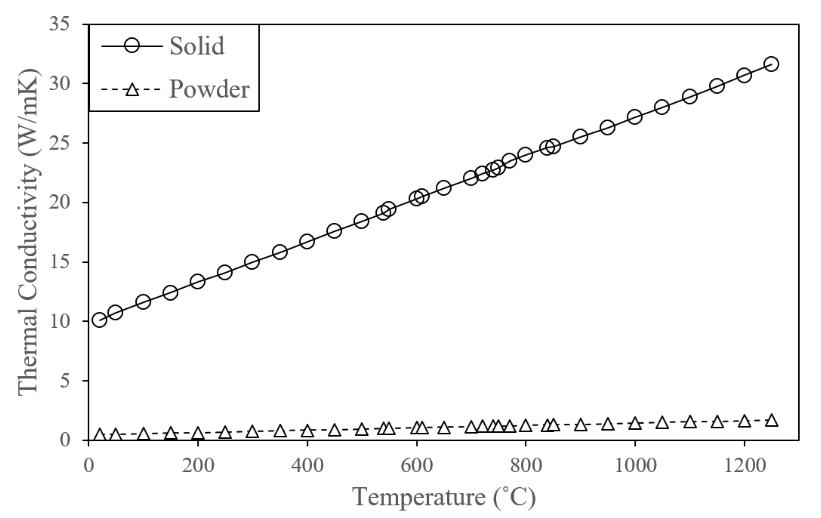
• A proper powder material model is used to calculate the temperature-dependent thermal conductivity incorporating the solid conductivity, the nitrogen gas conductivity, and the inter-particle radiation;
• The Marangoni effects inside the melt pool by calculating the Marangoni number and its equivalent thermal conductivity;
• Validation of the melt pool dimensions for single tracks with the literature;
• Experimental temperature measurement using a two-color pyrometer to validate the temperature from the multi-track layer model;
• In-depth RS profile measurement using XRD to validate the part scale model RS predictions;
• Study the effect of process parameters on thermal history, temperature gradients, CR, and their subsequent impact on the formation of RS.

2. Model Setup

2.1. Transient Thermal Model

Heat transfer in powder bed fusion is governed by heat conduction defined by the transient heat transfer energy balance equation, Equation (1)

$$k\left(\frac{{\partial }^{2}T}{\partial x^2}\right)+k\left(\frac{{\partial }^{2}T}{\partial y^2}\right)+k\left(\frac{{\partial }^{2}T}{\partial z^2}\right)+\dot{q}=\rho C\frac{\partial T}{\partial t}$$

(1)

where:

k: Thermal conductivity of the powder bed (W/m∙K)

T: Temperature (K)

$\dot{q}$: Energy generated per unit volume (W/m³)

$\rho$: Density of the powder bed (kg/m³)

C: Specific heat capacity (J/kg∙K)

t: time (s)

The initial condition for Equation (1) is set as the powder bed preheat temperature of 80 °C and represented by Equation (2)

$$T\left(x,y,z, t_0\right)=T_{preheat}$$

(2)

2.2. Boundary Conditions

2.2.1. Heat Flux Boundary Condition

As the laser beam irradiates the surface of the powder bed, heat is added into the powder, which can be represented as a specified heat flux boundary condition (BC) and defined using the Fourier heat flux equation given in Equation (3):

$$Q_{laser}=Q_{in}=k\nabla T\left(x,y,z\right)$$

(3)

2.2.2. Convection Boundary Condition

A constant nitrogen gas flow is pumped into the build chamber to reduce the oxygen percentage and carry away any spatter and ejected particles from the melt pool. The gas flow over the powder bed surface draws away heat due to forced convection, which is calculated using Equation (4):

$$Q_{convection}=h_o\left(T_{pb}-T_{\infty }\right)$$

(4)

where:

$h_o$: Overall heat transfer coefficient due to forced convection (W/m²∙K)

$T_{pb}$: Powder bed surface temperature

$T_{\infty }$: Ambient temperature (assumed 300 K)

The heat transfer coefficient due to forced convection is calculated similarly to the flow over a flat plate. Therefore, h will depend on the speed of the inert gas, as in Equations (6) and (7), and all fluid flow properties are to be calculated at film temperature [32,46]. The film temperature is the average temperature between the powder bed surface temperature and the gas flow temperature, Equation (5). The EOS M280 machine used to perform the experiments has an inert gas velocity of 3 m/s.

$$T_f=\frac{T_{pb}+T_{\infty }}{2}$$

(5)

$$h=\frac{k_g}{W}\frac{0.6776 R{e}^{1/2}P{r}^{1/3}}{\left[1+\frac{Pr}{0.0207}\right]}$$

(6)

$$Re=\frac{U_{\infty }W}{{\gamma }_g}$$

(7)

where:

$T_f$: The film temperature (K)

$k_g$: Gas thermal conductivity (W/m∙K)

W: Width of the powder bed (250 mm for EOS M280)

Re: Reynolds number calculated at the film temperature

Pr: Prandtl number

$U_{\infty }$: Inert gas velocity (m/s)

${\gamma }_g$: Kinematic viscosity (m²/s)

2.2.3. Radiation Boundary Condition

Another source of heat loss is radiation heat transfer to the surroundings, which is defined using Equation (8):

$$Q_{radiation}=e{\sigma }_s\left(T_{pb}{}^4-T_{\infty }{}^4\right)$$

(8)

where:

${\sigma }_s$: Stefan-Boltzmann constant (W/m²·K⁴)

$e$: Emissivity of the powder bed

Since the powder bed is porous, the bulk material properties cannot be used. Therefore, an analytical model is used to calculate the emissivity of the powder bed [47,48], represented by Equations (9)–(11).

$$e=A_H{\epsilon }_H+\left(1-A_H\right)e_s$$

(9)

$$A_H=\frac{0.908{\phi }^2}{1.908{\phi }^2-2\phi +1}$$

(10)

$$e_H=\frac{{\epsilon }_s\left[2+3.082{\left(\frac{1-\phi }{\phi }\right)}^2\right]}{{\epsilon }_s\left[1+3.082{\left(\frac{1-\phi }{\phi }\right)}^2\right]-1}$$

(11)

where:

$A_H$: Porous area fraction of powder surface

$\phi$: Powder bed porosity ratio

$e_s$: Emissivity of bulk material

The powder bed porosity depends on the recoating system and powder flowability [9]. However, it difficult to precisely measure the powder bed porosity and is usually assumed to be between 40% to 60%.

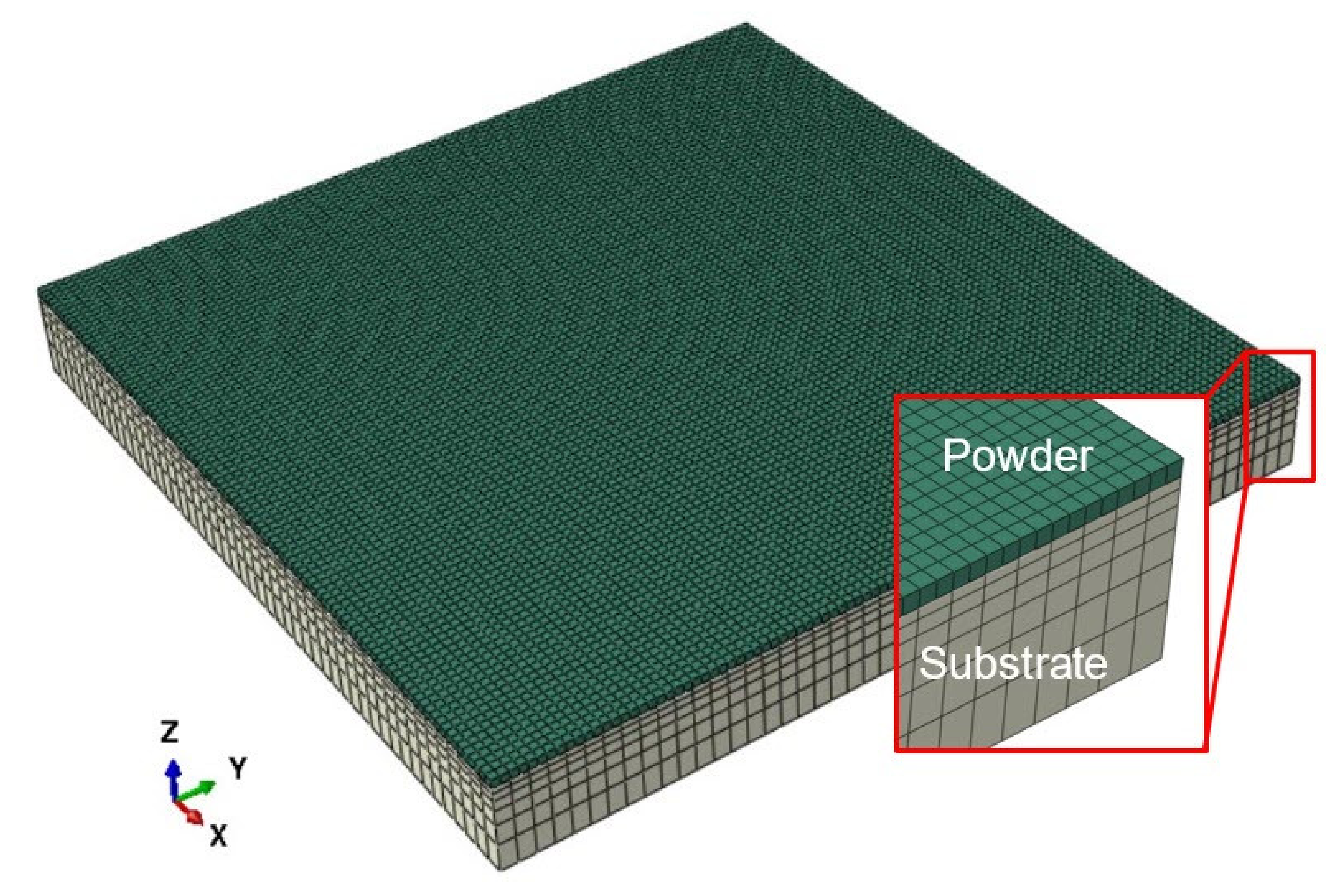
2.3. Material Model

In PBF, the powder is heated consistently up to melting. Therefore, the material model is governed mainly by the temperature-dependent thermophysical properties of the powder. An analytical model developed by Sih and Barlow [47] is used to calculate the thermal conductivity of the powder bed based on the bulk material thermal conductivity and powder bed porosity ratio. The model, Equation (12), considers the radiation between particles, Equation (13), and the presence of stagnant inert gas in the voids between the powder particles.

$$k_{pb}=k_g[\left(1-\sqrt{1-\phi }\right)\left(1+\phi \frac{k_r}{k_g}\right)+\sqrt{1-\phi } (\frac{2}{1-\raisebox{1ex}{$k_g$}\!\left/ \!\raisebox{-1ex}{$k_s$}\right.}\left(\frac{1}{1-\raisebox{1ex}{$k_g$}\!\left/ \!\raisebox{-1ex}{$k_s$}\right.}ln\frac{k_s}{k_g}-1)+\frac{k_r}{k_g})\right]$$

(12)

where:

$k_{pb}$: Powder bed thermal conductivity (W/m∙K)

$k_g$: Inert gas thermal conductivity (temperature dependent) (W/m∙K)

$\phi$: Powder bed porosity ratio

$k_s$: Thermal conductivity of the bulk material (temperature dependent)

$k_r$: Equivalent conductivity due to thermal radiation between powder particles

$$k_r=\frac{4\epsilon \sigma T^3{D}_p}{1-0.132\epsilon }$$

(13)

$e$: Emissivity of the powder (calculated previously)

T: Temperature (K)

$D_p$: Average diameter of the powder particles (m)

The next two properties to model powder bed thermal behavior are the specific heat capacity and density. A simplistic linear is used based on the porosity of the powder bed

$$C_p=\left(1-\phi \right)C_s$$

(14)

$${\rho }_p=\left(1-\phi \right){\rho }_s$$

(15)

The temperature-dependent thermo-physical properties of bulk IN625 were obtained from [49], and the full material properties used are shown in

Table 1. Thermo-physical properties of IN625.

Property		Units	Ref.
$\mathrm{Thermal}\mathrm{conductivity}(k_s)$	10.1–31.6	W/m∙K	[49]
$\mathrm{Density}\left({\rho }_s\right)$	8453–7925	Kg/m3	[49]
$\mathrm{Specific}\mathrm{heat}\mathrm{capacity}\left(C_{ps}\right)$	419–657	J/kg∙K	[49]
$\mathrm{Quescient}\mathrm{liquid}\mathrm{thermal}\mathrm{conductivity}\left(k_l\right)$	30.078	W/m∙K	[42]
$\mathrm{Liquid}\mathrm{specific}\mathrm{heat}\mathrm{capacity}\left(C_{pl}\right)$	709.25	J/kg∙K	[42]
$\mathrm{Solidus}\mathrm{temperature}\left(T_s\right)$	1563	K	[42]
$\mathrm{Liquidus}\mathrm{temperature}\left(T_L\right)$	1623	K	[42]
$\mathrm{Boiling}\mathrm{temperature}\left(T_b\right)$	3000	K	[42]
$\mathrm{Latent}\mathrm{heat}\mathrm{of}\mathrm{fusion}\left(L_f\right)$	290	kJ/kg∙K	[42]
$\mathrm{Latent}\mathrm{heat}\mathrm{of}\mathrm{vaporization}\left(L_V\right)$	640	kJ/kg∙K	[28]
Dynamics viscosity (μ)	$7\times {10}^{-3}$	Pa∙s	[42]
$\mathrm{Temperature}\mathrm{gradient}\mathrm{of}\mathrm{surface}\mathrm{tension}\left(d\sigma /dT\right)$	$-1.1\times {10}^{-4}$	N∙m/K	[28]
$\mathrm{Average}\mathrm{powder}\mathrm{size}\mathrm{diameter}\left(D_p\right)$	27	μm	[50]
Powder bed porosity (φ)	0.4	-	-
Emissivity (e)	0.4	-	[42]
$\mathrm{Nitrogen}\mathrm{thermal}\mathrm{conductivity}(k_g)$	0.02604–0.0947	W/m∙K	[51]
$\mathrm{Ambient}\mathrm{temperature}\left(T_{\infty }\right)$	313	K	-

.

The selection of a suitable material mode is essential to predict temperature history better. Since the primary mode of heat transfer in L-PBF is conduction, as mentioned above, a low thermal conductivity will lead to a high concentration of heat at the center of the melt pool and raise the predicted peak temperature. Employing the powder model shows that the solid thermal conductivity is 20 times the powder thermal conductivity, as shown in Figure 1.

2.4. Heat Source Modeling

A volumetric heat source model is employed to consider the laser beam penetration into the porous powder bed. Three models are chosen for comparison, the Goldak double ellipsoidal model, shown in Equation (16), which was developed for welding [52].

$$Q_v=\frac{6\sqrt{3}{A}_{c}P}{abc\pi \sqrt{\pi }}{e}^{-\left[\frac{3{\left(x-vt\right)}^2}{a^2}+\frac{3{\left(y-h\right)}^2}{b^2}+\frac{3z^2}{c^2}\right]}$$

(16)

where P is the laser power (W), $A_c$ is the absorption coefficient, x, y, and z are the local, a, b, and c are the longitudinal, transverse, and depth dimensions of the heat source, respectively, v is the laser scan speed (mm/s), t is the time (s), and h is the hatch spacing (mm). The dimensions a and b were assumed as the radius of the laser spot, while the depth dimension c is set as the melt pool depth determined experimentally.

The second and third heat source models examined are categorized as attenuated volumetric heat sources, based on the assumption that, as the laser penetrates the inter-particles voids, it becomes scattered and loses its energy at a certain depth. This attenuation depth is called the optical penetration depth (OPD), and its value was measured for pure nickel [53] at different powder particle size distributions (PSD), as shown in

Table 2. Optical penetration depth of pure Ni [53].

Particle Size Distribution	OPD
−20 μm	20 μm
−75 μm	200 μm

. However, there are no measured values for OPD in IN625 powders, but since IN625 comprises 58% Ni, the values for pure nickel were used to calculate the OPD using interpolation. The experiments were performed using an IN625 powder with a PSD of −45 μm [50], which gives an OPD of 100 μm.

The difference between the two attenuated volumetric heat sources is the attenuation profile being either a linear decay model, represented by Equation (17), or an exponential decay model, calculated using Equation (18).

$$Q_v=\frac{2A_{c}P}{\pi r^2}{e}^{\left[\frac{-2\left({\left(x-vt\right)}^2+{\left(y-h\right)}^2\right)}{r^2}\right]}\times \frac{2}{d}\left(1-\frac{z}{d}\right)$$

(17)

$$Q_v=\frac{2A_{c}P}{\pi r^{2}d}{e}^{\left[\frac{-2\left({\left(x-vt\right)}^2+{\left(y-h\right)}^2\right)}{r^2}\right]}\times e^{\left(-\frac{\left|z\right|}{d}\right)}$$

(18)

where P is the laser power (W), $A_c$ is the absorption coefficient, x, y, and z are the local, d is the OPD (mm), r is the laser spot radius (mm), v is the laser scan speed (mm/s), t is the time (s), and h is the hatch spacing (mm).

2.5. Melt Pool Modeling

The formation of a melt pool occurs in two steps: the first step occurs between the solidus and liquidus temperatures; hence, it is governed by the latent heat of fusion, given in Table 1. The second step is the fully melted phase, where fluid mechanics such as the Marangoni effect and natural convection dominate heat transfer in the melt pool. Marangoni effects are important, as they drive fluid flow inside the meltpool, hence altering its dimensions [54]. Additionally, the Marangoni effect will influence the solidification process and the resulting grain formation [55,56]. Simulation of the Marangoni effect requires the use of CFD; however, the current study employs an FE model to predict the RS. In order to overcome the absence of fluid flow modeling in FE, an effective thermal conductivity model [57] is used to account for heat transfer due to the Marangoni effect artificially, as shown in Equation (19).

$$k_{eff}=k_l+hL$$

(19)

where $k_{eff}$ is the effective thermal conductivity (W/m·K), $k_l$ is the quiescent liquid thermal conductivity (W/m·K), h is the convective heat transfer coefficient (W/m²·K), and L is the characteristic length (m), which is assumed as half the melt pool width [57,58]. The value of the convective heat transfer coefficient inside the melt pool can be calculated from the Nusselt number using Equation (20), which is the ratio of convective to conduction heat transfer. Since convection in the melt pool is driven by the Marangoni effect, then the Nusselt number can be calculated as a function of the Marangoni number shown in Equations (21) and (22).

$$Nu=\frac{hL}{k_l}$$

(20)

$$Nu=1.6129ln\left(Ma\right)-10.183$$

(21)

$$Ma=-\frac{d\sigma }{dT}\frac{L\Delta T\rho C_{pl}}{\mu k_l}$$

(22)

where Nu is the Nusselt number, Ma is the dimensionless Marangoni number, $\frac{d\sigma }{dT}$ is the temperature gradient of surface tension (N·m/K), L is the characteristic length, ρ is the liquid density (kg/m³), $C_{pl}$ is the liquid specific heat capacity, $k_l$ is the quiescent liquid thermal conductivity (W/m·K), μ is the dynamic viscosity (kg/m·s), and $\Delta T$ is the maximum temperature gradient in the melt pool, which is taken as the temperature difference between the center of the melt pool (peak temperature) to the boundary of the melt pool (solidus temperature) and is calculated using Equation (23)

$$\Delta T=\frac{-C_{pl}+\sqrt{C_{pl}{}^2+2{\left(\frac{d\sigma 1}{dT\mu }\right)}^{2}dt\frac{Q_v}{\rho }}}{{\left(\frac{d\sigma 1}{dT\mu }\right)}^2}$$

(23)

$$dt=\frac{L}{v}$$

(24)

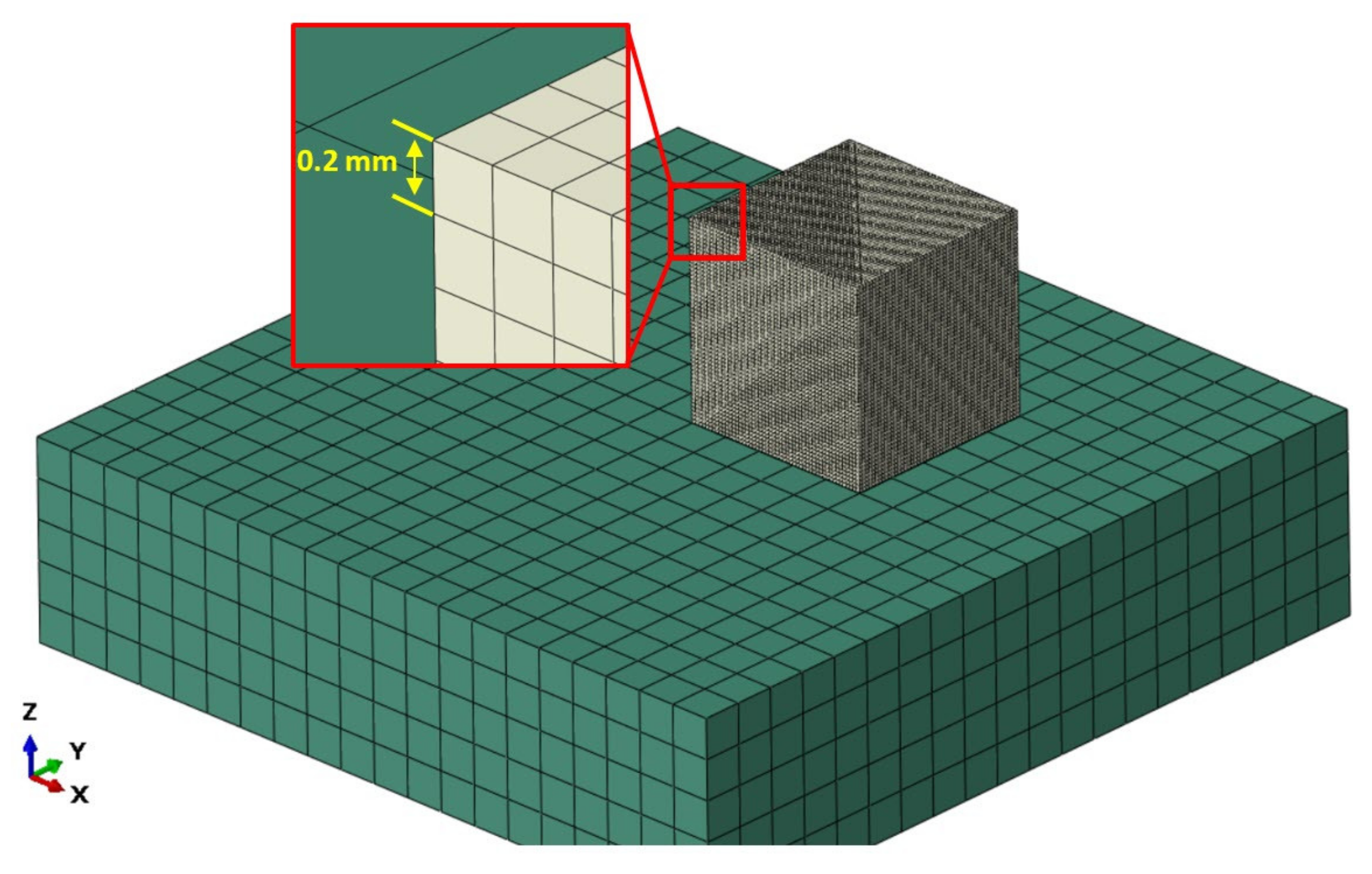
2.6. Modeling Approach

The modeling approach is based on three models, each focusing on predicting a certain set of results to characterize the thermo-mechanical response occurring in L-PBF under different process parameters. The first model is a single-track model, with a very fine mesh, to test the validity of the proposed material, melt pool, and heat source models by predicting melt pool dimensions, temperature gradients, and CR and comparing them to experimental results. The second model is a layer scale model with a coarser mesh to simulate the effects of multi-tracks on the temperature history, CR, melt pool dimensions, and the subsequent RS evolution in a single layer. The third model is a low-fidelity part scale model, which examines the far-field temperature histories and how it drives the final in-depth RS and part distortion.

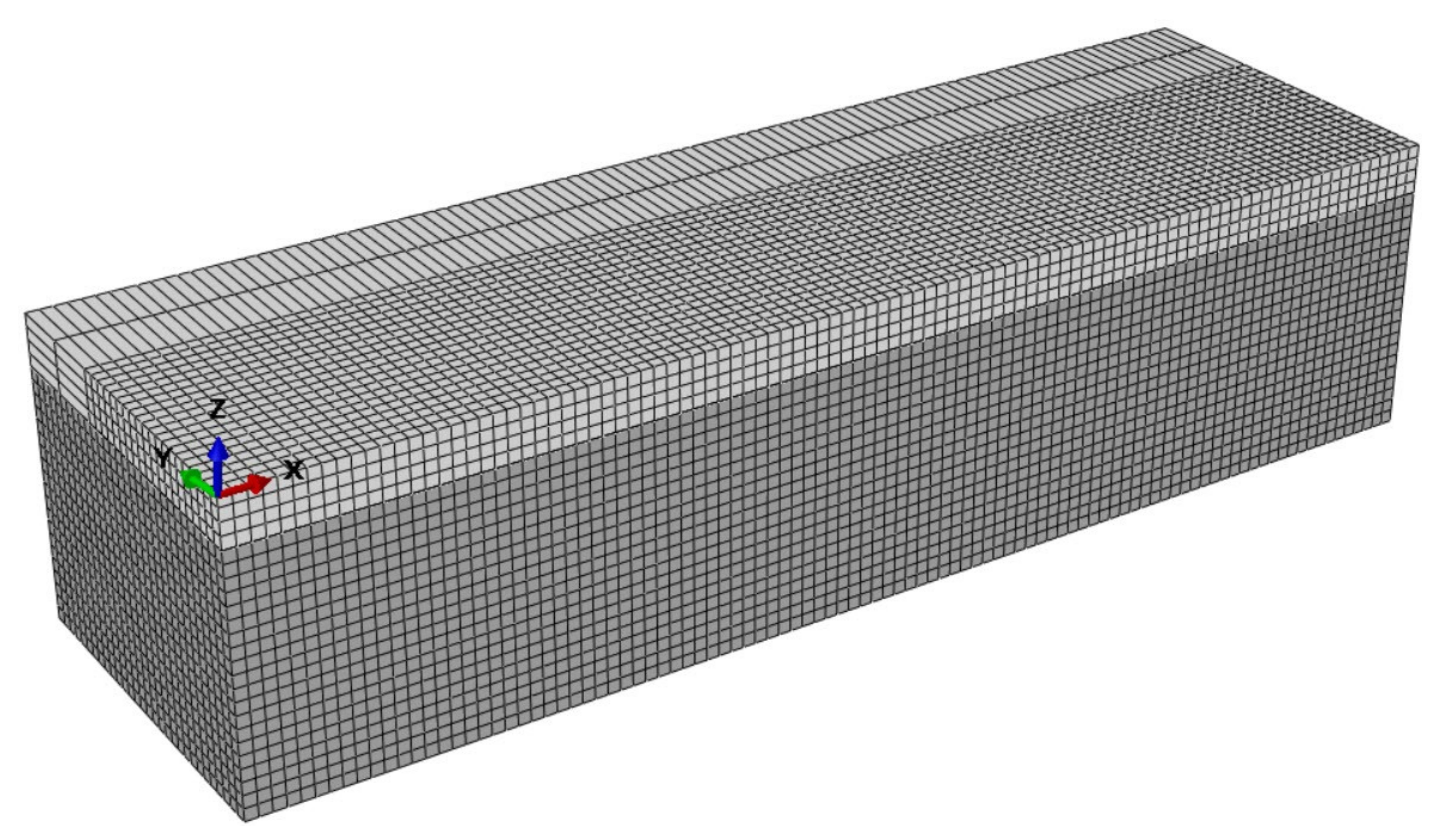
2.6.1. Single-Track Model

A 3D Lagrangian finite element (FE) model was built using ABAQUS to model single-track exposure of IN625. The model dimensions are 1 mm × 240 μm × 300 μm, with the top 40 μm assigned as the powder layer, as shown in Figure 2. The model was meshed with heat transfer DC3D8 elements with a minimum size of 10 μm employed in the powder layer. The volumetric heat flux was applied as a body on the powder layer using the user subroutine DFLUX to simulate the spatial movement of the laser beam with time. Symmetry BC was assigned to reduce the model’s size, with the XZ plane taken as the plane of symmetry.

The user subroutine USDFLD changes the material model from powder to liquid and then to solid as the material solidifies. The criteria for changing the material state depends on the condition of reaching the melting temperature, as shown below:

$$Material state variable \left(SV\right)=\left\{\begin{array}{c}0\to Powder T<T_{melt}\\ 1\to liquid T>T_{melt}\\ 2\to Solid T < T_{melt} and T_{max} > T_{melt}\end{array}\right.$$

The melt pool dimensions, temperature gradient, and CR are extracted from the model when the melt pool reaches a steady-state, determined when the peak temperature reaches a constant value. The process parameters studied include two laser powers, 140 W and 220 W, and two scan speeds, 500 mm/s and 650 mm/s.

2.6.2. Multi-Track Model

The multi-track model aims to observe the effect of hatch spacing, laser power, and scan speed on the temperature profile, temperature gradient, CR, and consequent effect on RS evolution during the solidification layer. In order to do so, a sequentially coupled thermal stress model is used, since, in LPBF, the temperature change will drive a change in stress, but the generation of stress will not cause an increase in temperature. Therefore, two separate models, 3D FE models, were built: firstly, a pure heat transfer model to calculate the temperature fields generated due to laser exposure. Secondly, the temperature fields from the heat transfer model were imported into a static stress model to calculate the thermal stresses developed due to the cooling down of the material during solidification.

The heat transfer model has a powder layer with dimensions of 4 mm × 4 mm × 0.04 mm and is tie-constrained to the substrate having a thickness ten times the powder layer. The model was meshed with DC3D8 hexahedral elements having a uniform size of 40 μm. In contrast, the substrate had a coarser mesh with the element size biased towards the top surface, where the element size starts at 40 μm and increases to 140 μm, as shown in Figure 3. The user subroutine USDFLD changed the powder layer’s material properties from powder to liquid and solid material due to material heating, melting, and cooling.

The scan strategy employed was a stripe scan with serpentine laser motion [50]. The laser heat load was defined as a body flux acting on the powder layer, and the spatial motion of the laser beam was implemented using the DFLUX subroutine. The step time was set as the total time required to expose a layer with a cross-section of 10 mm × 10 mm, the same size as the experiments [50]. The laser process parameters are stated in

Table 3. Process parameters for LPBF of IN625.

Parameter	Levels
Power (W)	140, 220, 270
Scan speed (mm/s)	500, 650, 800
Hatch spacing (mm)	0.08, 0.1, 0.12

. A preheat temperature of 80 °C was assigned to the whole model and set as a BC for the bottom surface of the substrate. Convection and radiation are defined for the top surface of the powder layer with an ambient temperature of 40 °C. The temperature profiles, temperature gradients, and CRs are extracted at the center point of the powder layer to examine the effect of multi-track laser exposures and hatch spacing on temperature evolution.

The static stress model had the same dimensions and mesh size as the heat transfer model. Thermal stresses are the main driver of RS and deformation in LPBF; hence, the temperature field from the heat transfer model was assigned as an initial condition in the stress model. Since LPBF is characterized by rapid cooling, the molten material solidifies once the laser beam passes. This means that solidification and stress formation progressively follow the laser beam during the multi-track exposure. Therefore, to model this behavior, “quiet” or “inactive” elements represented the powder material that did not develop any stresses yet. Once the laser beam passes over these elements, they are activated to calculate stress evolution during cooling. The user subroutine UEPACTIVATIONVOL was used for progressive activation of the powder layer elements in tandem with the laser scan strategy. The coordinates of the laser position are calculated at every increment, and the elements within a circle, with a diameter equal to the melt pool width calculated from the heat transfer model, are activated [59]. Due to a limitation in Abaqus, a set of elements with an area equal to the laser spot diameter needed to be activated priory to avoid convergence issues with UEPACTIVATIONVOL. In order to reduce computational time and improve the convergence of the non-linear model, the unsymmetric stiffness matrix storage option is selected to use Newton’s method to solve the non-linear problem. In addition, the strain state extrapolation feature is turned off to improve convergence [60,61].

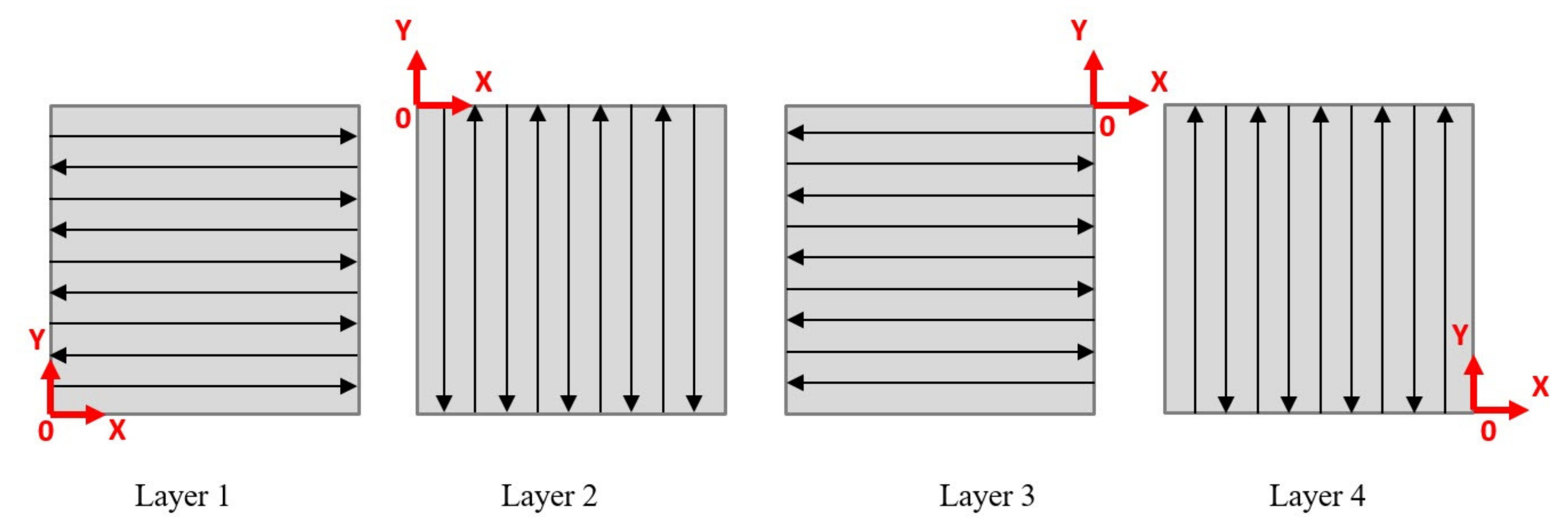
2.6.3. Multi-Layer Model

A large-scale FE model is required to predict stresses and deformations on a part scale. However, utilizing a fine mesh from the high-fidelity model would be computationally infeasible. Therefore, a low fidelity model that predicts the far-field temperatures without focusing on the melt pool area during printing and recoating was proven to provide good predictions of part scale stresses and deformations [17,61]. The ABAQUS AM module [62] was used to build the sequentially coupled temperature-stress part scale model, consisting of a heat transfer step followed by a stress analysis step, and finally removing the part from the build plate.

The heat transfer model consists of a 10 mm × 10 mm × 10 mm cube coupon meshed with DC3D8 200 μm elements, while the substrate has a coarser mesh of 2 mm in size, as shown in Figure 4. The 200 μm element used is a lump sum of five layers of 40 μm thickness to save on computational cost, since the interest is the far-field temperature history [17,61]. The part and the substrate are connected using a “tie-constraint.” Simulation of the PBF process requires successive addition of material using UEPACTIVATIONVOL subroutine based on an event series that specifies the time instances where the recoating starts and ends. A Matlab code was written to generate the recoater event series file, with the recoating time set at 5 s. The laser heat source is modeled as a point source, which is acceptable when the laser spot size is relatively smaller than the element size. A stripe scan with serpentine laser motion was used for in-layer exposure, while a 0°–90°, alternating scan was employed for subsequent layer exposures, as illustrated in Figure 5. An event series data set is created using Matlab to determine the time, spatial coordinates, laser power, and laser spot diameter corresponding to the employed scan strategy. The tool path–mesh intersection built-in module determines the intersection of the laser event series with the element integration points and then calls the user subroutine UMDFLUX to apply heat flux at the corresponding time [61,62]. The newly formed external surfaces are automatically determined, and the radiation and convection heat transfer is applied. Finally, after the whole part is exposed, it is left to cool down for 600 s.

The same geometry and mesh size were used for the stress analysis model, where the temperature fields from the heat transfer model are imported into the stress model. The thermal strains and stresses were calculated by imposing an initial temperature of 1000 °C, above which thermal stress is negligible. The difference between this temperature and the imported part temperature will determine the thermal stress field [17,61]. Temperature-dependent material properties were used [49,63], while Johnson–Cook (J–C) plasticity [64] was used to model the temperature-dependent plasticity according to Equation (25):

$$\sigma =\left(A+B{\epsilon }^n\right)(1+Cln(\frac{\dot{\epsilon }}{\dot{{\epsilon }_o}}))(1-{\left(\frac{T-T_r}{T_m-T_r}\right)}^m)$$

(25)

where $\sigma$ is the von mises flow stress, $\epsilon$ is the equivalent plastic strain, $\dot{\epsilon }$ is the equivalent plastic strain rate, and $\dot{{\epsilon }_o}$ is the reference plastic strain rate. T is the current temperature, $T_m$ is the melting temperature, and $T_r$ is the reference temperature at which the J–C parameters were determined. A is the initial yield strength, B is the strain hardening coefficient, n is the strain hardening exponent, C is the strain rate coefficient, and m is the thermal softening exponent. The values for the J–C parameters used in the current study are listed in

Table 4. Johnson–Cook plasticity parameters [65].

Parameter	Value
A (MPa)	558
B (MPa)	2201.3
n	0.8
C	0.000209
m	1.146
Tm (°C)	1290
Tr (°C)	20
$\dot{{\epsilon }_o} \left(s^{-1}\right)$	1670

.

The J–C parameters listed above were determined for a conventionally manufactured IN625; in an attempt to partially modify these parameters to match that of the additively manufactured IN625, a tensile test was performed at room temperature. A sub-size flat specimen was printed with dimensions according to the ASTM E8 standard [66] with a gauge length of 25 mm, a width of 6 mm, and a thickness of 5 mm. The true stress–strain curve was plotted, and the Ramberg–Osgood model [67] was used to fit the data according to Equation (26) and calculate the yield strength, the strength coefficient (K), and the strain hardening exponent (n), which are analogous to the A, B, and n parameters in the J–C equation.

$${\epsilon }^{total}=\frac{{\sigma }_y}{E}+{\left(\frac{\sigma }{K}\right)}^{\raisebox{1ex}{$1$}\!\left/ \!\raisebox{-1ex}{$n$}\right.}$$

(26)

A total fixation BC is applied to the bottom surface of the substrate. After the part was built and cooled down, the substrate was removed using the model change feature to simulate the part’s separation from the substrate. The substrate removal will release some stresses, and the RS inside the part will remain. For validation, the stresses are extracted and averaged across an area 2 mm in diameter to resemble the spot size of the experimentally measured RS using XRD measurement.

3. Experimental Validation

3.1. Laser Absorptivity Measurement

Diffuse reflectance spectroscopy (DRS) was used to measure the optical absorptivity of the IN625 in a wavelength range of 400–1400 nm. The test measures the powder’s reflectance, which is used to calculate the Kubelka–Munk absorption coefficient, as shown in [9]. For example, for an EOSM280, the Yb-fiber laser used has a wavelength of 1070 nm that corresponds to an absorptivity coefficient of 0.62.

3.2. Single Track Validation

The melt pool width and depth predicted by the single-track model are validated by comparing them to the experimental melt pool dimensions measured in the literature [68,69]. The single exposed by NIST [68] and Dilip et al. [69] were built with a layer thickness of 20 μm, and the model geometry was modified to accommodate the smaller layer thickness. The meltpool dimensions were measured by extracting the distance from the center of the melt pool to the outer temperature contour having a temperature corresponding the solidus temperature of 1290 °C.

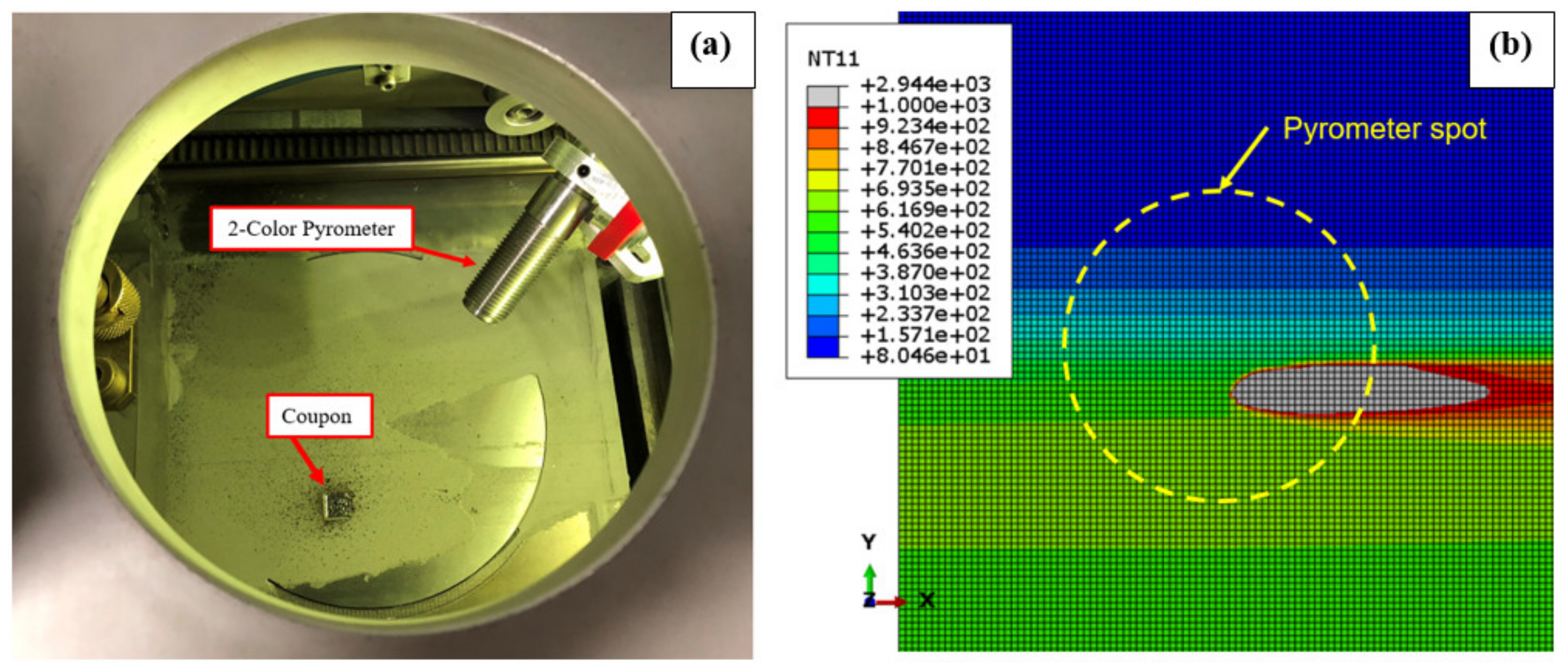
3.3. Multi-Track Temperature Measurement

A Fluke Endurance-series two-color pyrometer was used to measure melt pool measurements during exposure of a single layer. The two-colour pyrometer operation is based on the ratio of two separate infrared bands with a slight difference in wavelength to determine the object’s temperature. Hence, temperature measurement would be independent of the emissivity, thus reducing measurement uncertainty. The pyrometer used has a Si/Si detector with a nominal wavelength of 1 μm, and the ratio between the two wavelengths, also called the slope, was calibrated as 0.96 [70]. The pyrometer has a temperature range of 1000–3000 °C, and it was installed inside the build chamber of an Omnitek L-PBF machine, as shown in Figure 6a, at a distance of 85 mm, which results in a measurement spot size of 2 mm in diameter.

For validation, the elements temperatures above 1000 °C, i.e., the lower limit of the pyrometer, within a 2 mm diameter circle were averaged and compared to the pyrometer measurements [71], as shown in Figure 6b. The tested parameters were 220 W, 650 mm/s, 0.12 mm hatch spacing, and a layer thickness of 0.04 mm. Since the pyrometer had a response time of 10 ms, the temperatures calculated from the model are extracted and averaged at an increment of 10 ms.

3.4. Residual Stresses Measurements

In-depth RS were measured in IN625 cube coupons [50] using X-ray diffraction (XRD). Since X-ray penetration depth is about 5 μm in Inconel, electro-polishing was used to minimally affect the existing stress field [72]. The material was removed in 0.1 mm increments down to a depth of 1 mm from the top surface. RS were measured in two directions; parallel to the laser motion (scan direction) and perpendicular to it (hatch direction). The in-depth RS measurements were performed on two samples corresponding to two laser powers, 140 W and 220 W, at a hatch spacing of 0.12 mm, and a constant scan speed of 650 mm/s. In addition, predicted RS is compared to surface RS measured by the current authors in a previous study [50] at different process parameters.

4. Results

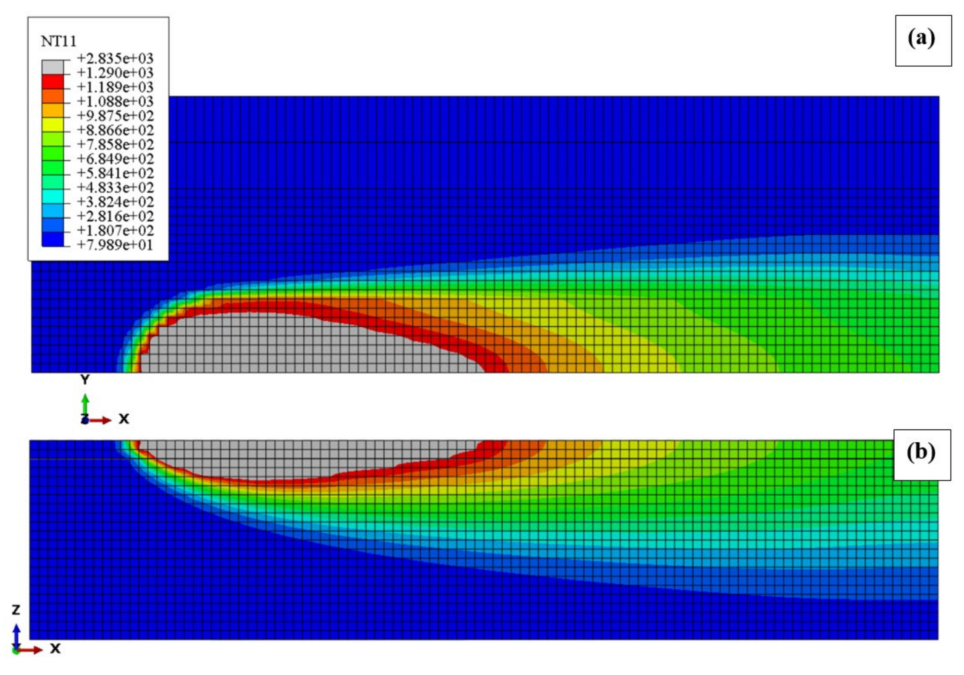
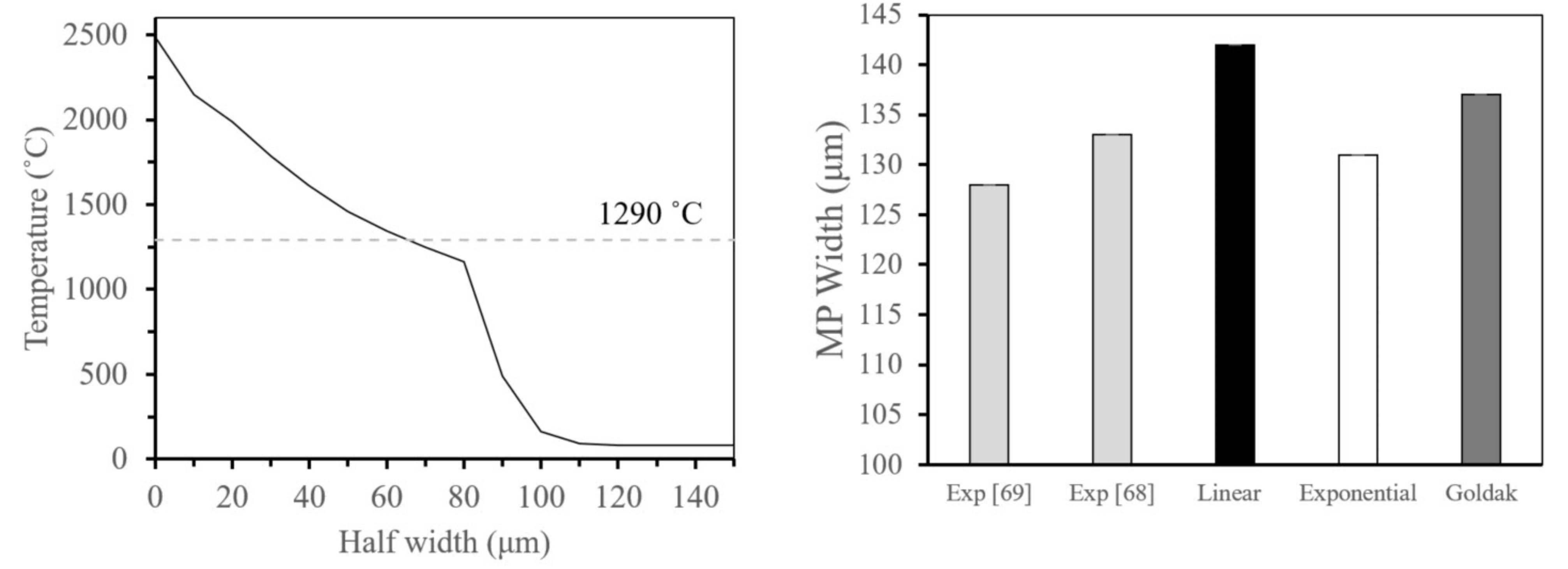
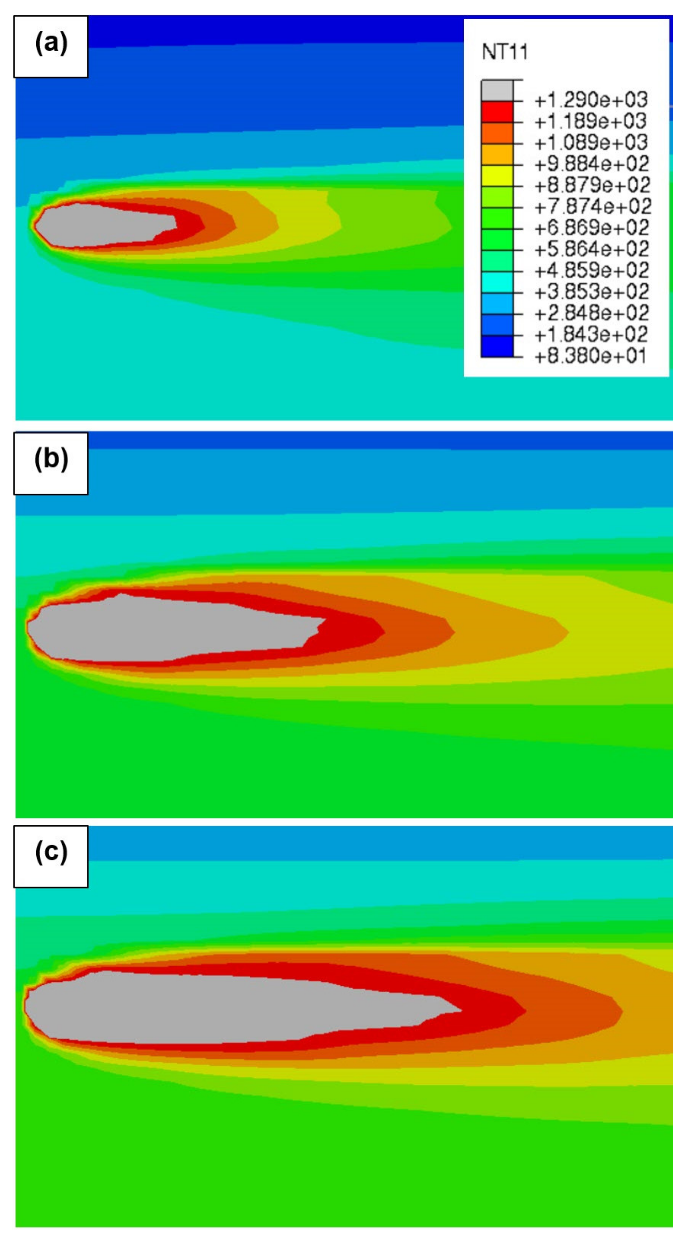
4.1. Single Tracks

The temperature contours of the predicted melt pool are shown in Figure 7 for the 20 μm layer thickness validation model with an exponential heat source. The grey-colored area represents temperatures above the solidus temperature of 1290 °C. The temperature profiles are plotted in the width direction, Figure 8, and in-depth, to calculate the melt pool dimensions, as shown in Figure 9. The intersection point of the temperature profiles with the solidus temperature locus determines the width and depth of the melt pool.

Comparison of the experimentally measured melt pool width [68,69] with the predicted melt pool width for the three heat source models is shown in Figure 8. The exponential heat source model predicted a melt pool width of 131 μm, which best agrees with the experimental measurements. However, the melt pool depth was underestimated for all three heat source models, as shown in Figure 9. The melt pool depth measured by NIST [68] was much deeper than the predicted value due to printing on the bare substrate without a powder layer. Therefore, the exponential heat source was chosen for subsequent simulations. The length of the melt pool was measured in the study by NIST [68] using a high-speed infrared camera. By comparing the result with the numerical prediction, Figure 10 shows that the model greatly underestimates the melt pool length. The underestimation could be attributed to approximating the Marangoni effect inside the melt pool and calculating its value based only on the outward flow in the melt pool width direction.

Calculating the melt pool width and depth for the parameters examined in the current study (Figure 11) shows that the melt pool dimensions decrease with increased scan speed, which agrees with the literature [68,69,73]. Furthermore, it is observed that the melt pool width is inversely proportional to the square of the scan speed, while the melt pool depth is inversely proportional to the scan speed.

The temperature history is extracted at the midpoint along the laser scan path and plotted, as an example, for the case of 220 W and 650 mm/s, as shown in Figure 12. A rapid temperature rise is seen as the laser approaches the midpoint, followed by rapid cooling to 1290 °C. Finally, the CR is calculated as the slope of the temperature history profile once the temperature drops below the solidification temperature, which will drive RS.

The CR for all three scan speeds is plotted in Figure 13 and is to the order of 10⁵, characteristic of rapid cooling. The cooling increases linearly with increasing scan speed, regardless of the laser power. The temperature gradient is also plotted in Figure 13, as it affects the magnitude of thermal stresses formed during cooling according to Equation (27), where E is the modulus of elasticity (MPa), $\alpha$ is the thermal expansion coefficient, and $\Delta T$ is the temperature gradient (°C).

$$\sigma =E\alpha \Delta T$$

(27)

The temperature gradient exhibits a downward trend with increased scan speed, resulting in RS with the same trend. However, previous experimental RS measurements show non-monotonic trends for RS values [50]. These trends could mean that RS is governed by a temperature gradient, and the opposite effect of CR could play a role in determining the final stress state [42].

4.2. Multi-Track Model

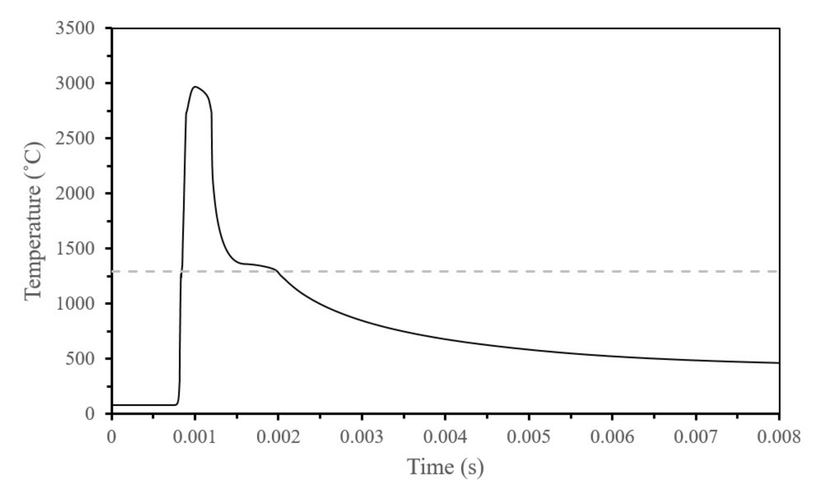
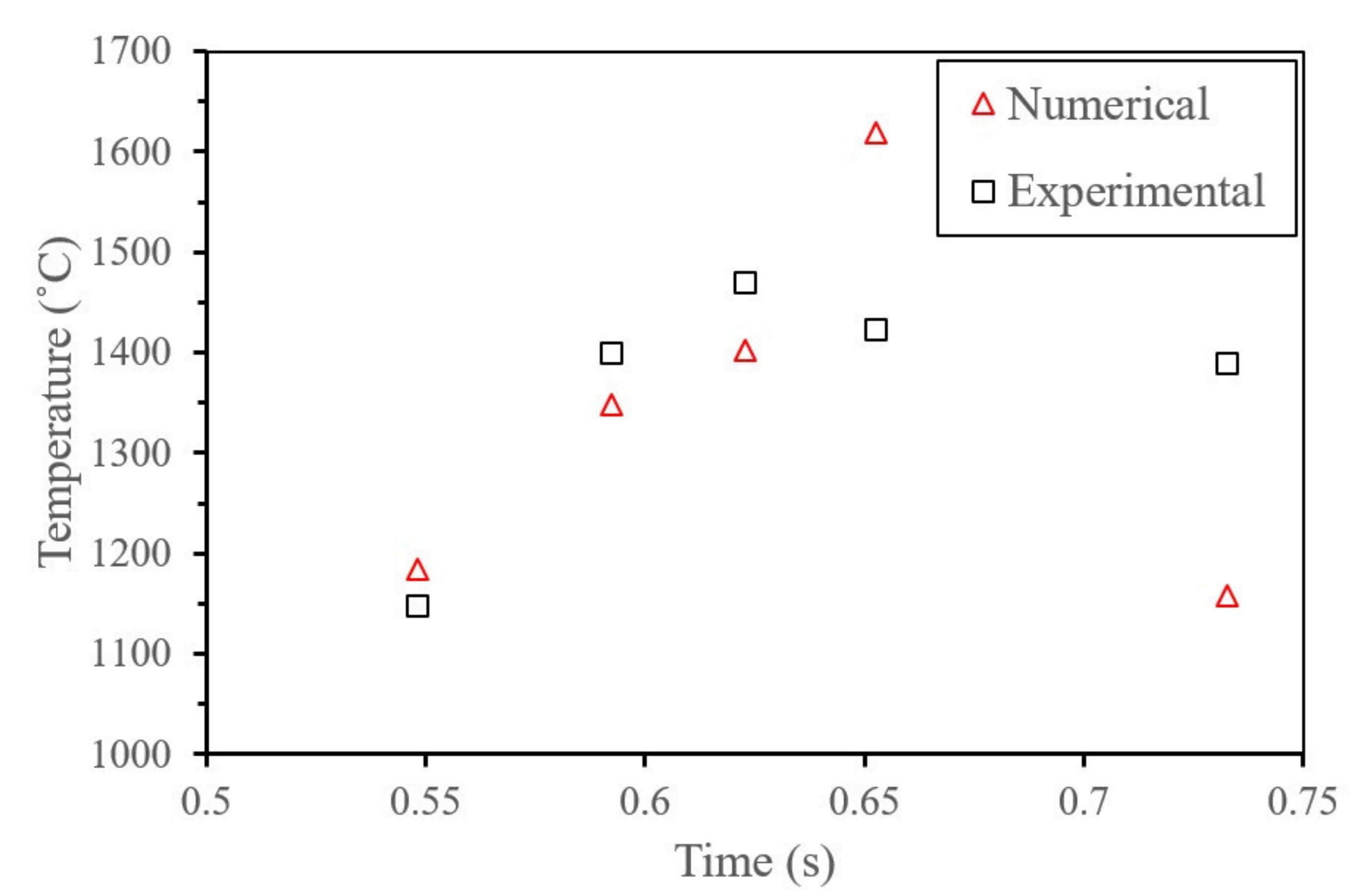
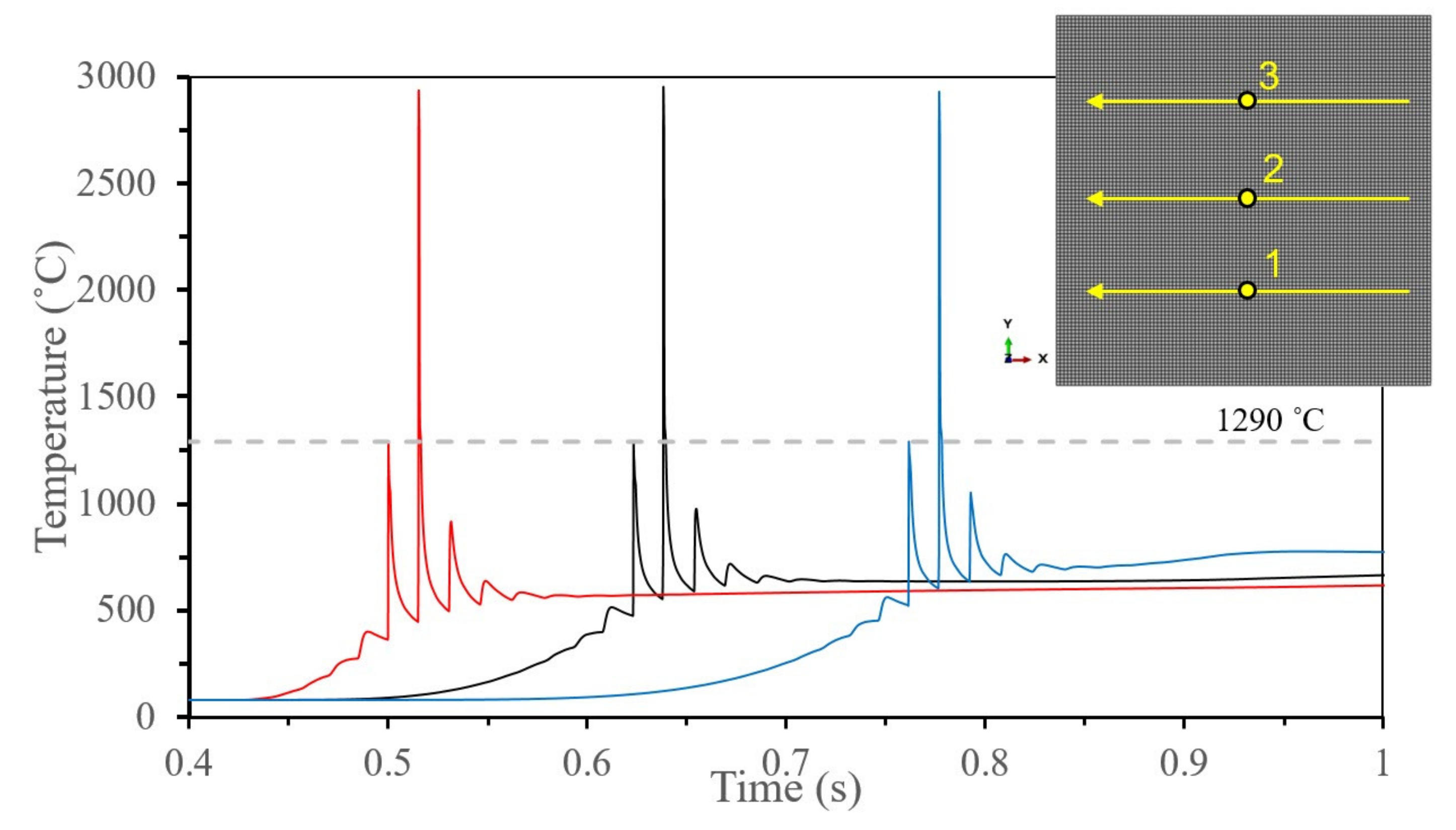
4.2.1. Temperature Validation and Evolution

Temperature predictions from the multi-track model are compared to pyrometer measurements, as shown in Figure 14. The numerical temperature predictions are in good agreement with the experimental data. However, the discrepancy at the highest temperature predictions could be due to underestimating the melt pool length; since the calculated temperature is averaged over the melt pool, a difference in the melt pool area will affect temperature prediction.

The temperature history is plotted at three points, 1 mm apart, at 220 W laser power, 650 mm/s scan speed, and 0.12 mm hatch spacing, as shown in Figure 15. The three points exhibit the same thermal cycles where the temperature rises to a point shy of the melting temperature as the laser scans the precedent track. Afterward, the temperature at the point of interest cools down to about 500 °C as the laser beam passes directly over it, resulting in a peak temperature higher than the boiling temperature. Due to rapid cooling, the temperature drops from 2900 °C down to 570 °C, where the heat from the subsequent track scan causes the temperature to rise again to 950 °C. Beyond that point, the temperature drops to a plateau of about 650 °C until the whole layer is scanned. The CR and temperature gradients are plotted in Figure 16 for the points mentioned above. The presented CR is calculated as the temperature cools down below 1000 °C. Although a larger surrounding solid area could indicate that the cooling will increase because the solid material has higher thermal conductivity and specific heat capacity compared to the powder state, it is shown that the CR decreases as the area of the solidified layer increases. The reason is that the larger solidified volume retains more heat; therefore, the area surrounding the melt pool has a relatively high temperature, resulting in a lower temperature gradient, as shown in Figure 16, and lower heat transfer due to conduction.

In addition, Figure 17 compares the temperature and von Mises stress evolutions during the layer exposure at different time instances until the end of exposure at 1.25 s. The peak temperatures are mainly focused inside and around the boundary of the melt pool and drastically decay beyond that. Conversely, the Mises stress is minimum around the melt pool boundaries and increase farther away from the melt pool due to the rapid cooling and stress generation, until it reaches its maximum value at the part edges, as seen in Figure 17f.

The temperature evolution at the midpoint of the modeled area is plotted in Figure 18 for the total layer time of 6.25 s, corresponding to 1.25 s of laser exposure plus 5 s for powder recoating. The temperature profile can be divided into a rapid non-linear phase, which occurs during the first 1.25 s, followed by the linear phase. The thermal stresses are also plotted for the principal directions, the laser scan direction (S11), and the perpendicular direction, the hatch direction (S22), where S11 is observed to be always greater than S22. To understand why S11 is greater than S22, the RS formation mechanism needs to be explained.

RS in LPBF is formed due to the difference in thermal strains during subsequent heating and cooling during subsequent scans called the temperature gradient mechanism (TGM) [15,73,74], governed by Equation (27). To better understand the formation mechanism of RS, Figure 19 shows a layer during laser exposure where the yellow area, $A_T$, represents a track along the laser path surrounded by the previously solidified area, $A_S$, and the subsequent powder area. This layer can be represented by the bar model analogy for simplification, whereas bar T and S are constrained at one end and free to move on the other end. As bar T is heated, it expands and pulls on bar S, resisting the motion by inducing compressive stress. The stress cycle undergone by the material is represented by the stress-temperature plot in Figure 19, where the compressive stress increases with temperature till reaching the yield temperature $\left(T_y\right)$ at point A, upon which plastic deformation occurs. As bar T cools down during solidification, the compressive strains and stresses decrease to zero at point C. As the temperature drops further, bar T shrinks and pulls on bar S, which resists this motion; therefore, bar T experiences tensile strains while bar S exhibits compressive strains. Finally, the tensile stress in bar T increases up to the yield point, where the material undergoes another plastic deformation until reaching equilibrium temperature. These plastic strains lock in the thermal stresses and prevent them from returning to zero, thus creating RS. The RS can be represented by Equation (28) or Equation (29), depending on the maximum temperature experienced by the material.

If $T_y\le T_{max}<2T_y$, then

$${\sigma }_{RS}=\left|E\Delta {\epsilon }_{p1}\right|=\alpha E\left(T_{max}-T_y\right),$$

(28)

If $2T_y\le T_{max}$, then

$${\sigma }_{RS}=\left|E\Delta {\epsilon }_{p1}+E\Delta {\epsilon }_{p2}\right|=\alpha E{T}_y$$

(29)

The same bar model analogy can be used to explain why S11 is greater than S22 by examining Figure 20, where the bar model is superimposed on arbitrary melt pool temperature contours [75]. The thermal stress in the X direction (S11) is generated due to the temperature difference with the adjacent area in the Y direction $\left(\Delta T_Y\right)$, while the thermal stress in Y direction (S22) arises due to the temperature difference in the X direction $\left(\Delta T_X\right)$. As shown in Figure 16, $\left(\Delta T_Y\right)$ is always greater than $\left(\Delta T_X\right)$; hence, S11 is always greater than S22.

Figure 21 provides a closer examination of the non-linear stress formation phase, where the material undergoes a few heating and cooling cycles. Commonly, stresses that are generated due to a moving heat source were considered to be affected by the temperature gradient only and its thermal softening effect on the material. However, in LPBF, the material deforms at high strain rates due to the high CR, which causes strain rate hardening, thus opposing the thermal softening effect. Following the temperature and stress evolution in Figure 21, it is seen that the stress is zero as long as the temperature has not reached the melting temperature; hence, it remains in its powder state. As the laser passes over the point of interest during track n, the material melts, and as it solidifies, stresses are generated. By examining Figure 21 and Figure 22 simultaneously, to observe the stress and plastic strain formation during cooling, it is seen that as the temperature decreases, the compressive plastic strain decreases, analogous to line BD in Figure 19, while tensile stresses increase. As the laser beam exposes track n + 1, the conducted heat causes a temperature rise of track n, as mentioned previously, thus causing an increase in compressive stress and a corresponding decrease in tensile stresses. Finally, the temperature due to the conducted heat reaches a maximum of 940 °C, the material cools down again, generating more tensile stresses. As the distance between track n and laser spot increases, the quantity of heat reaching track n decreases. Therefore, the material undergoes low peak heating and cooling cycles, which generates comparatively lower tensile stresses.

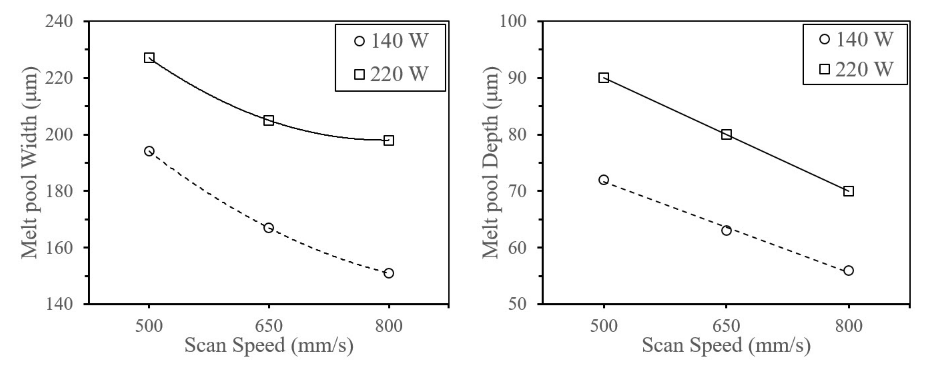
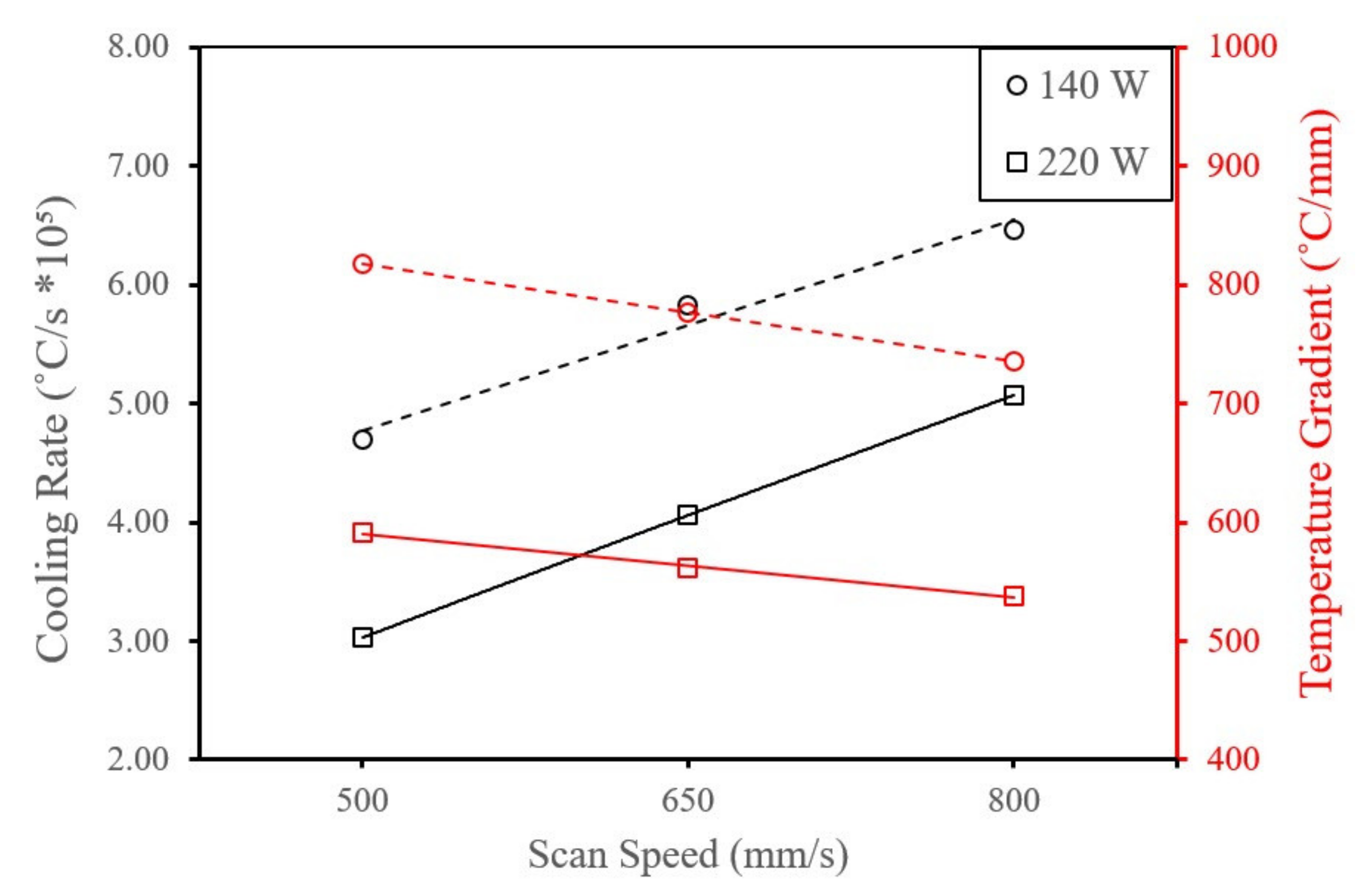
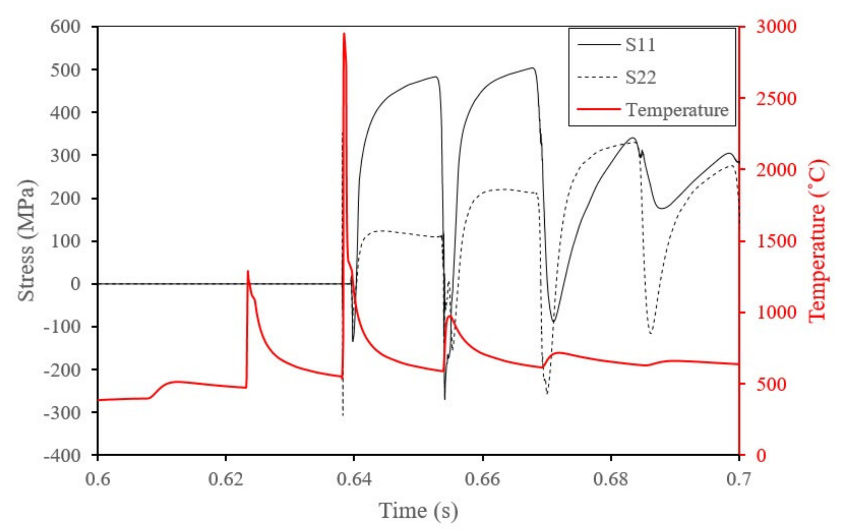
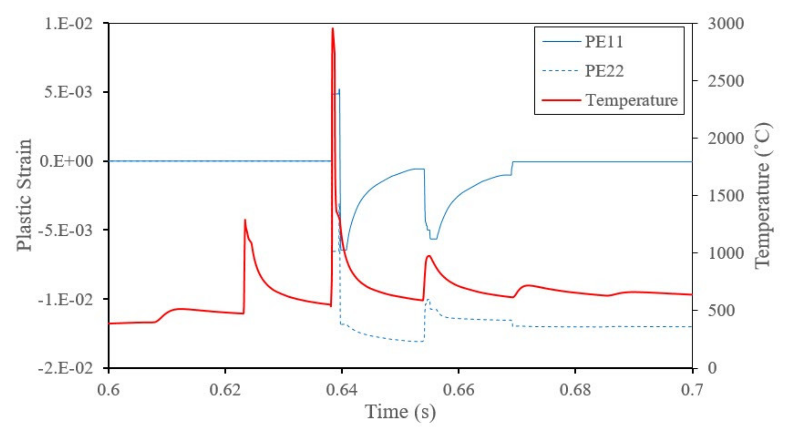
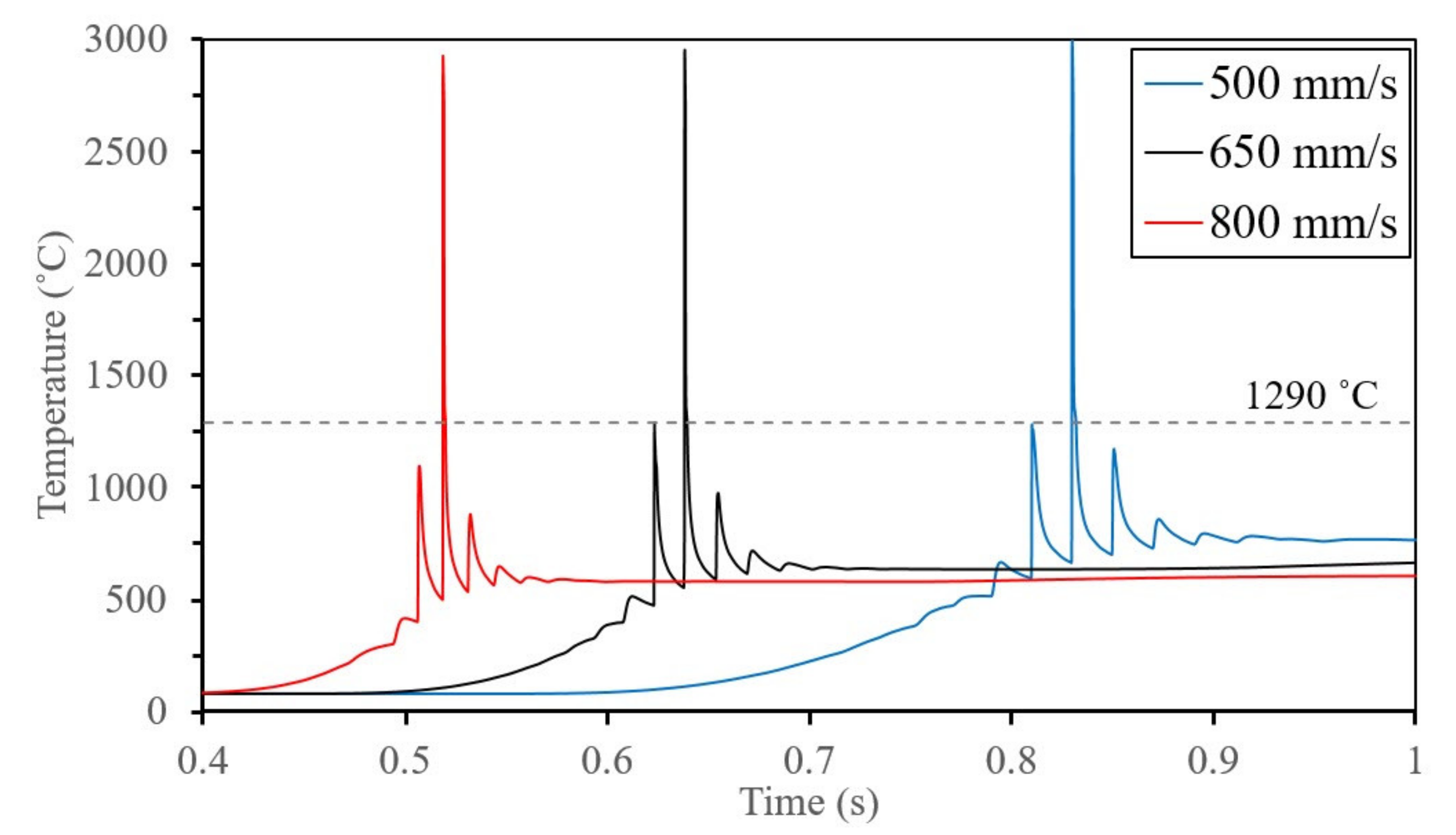
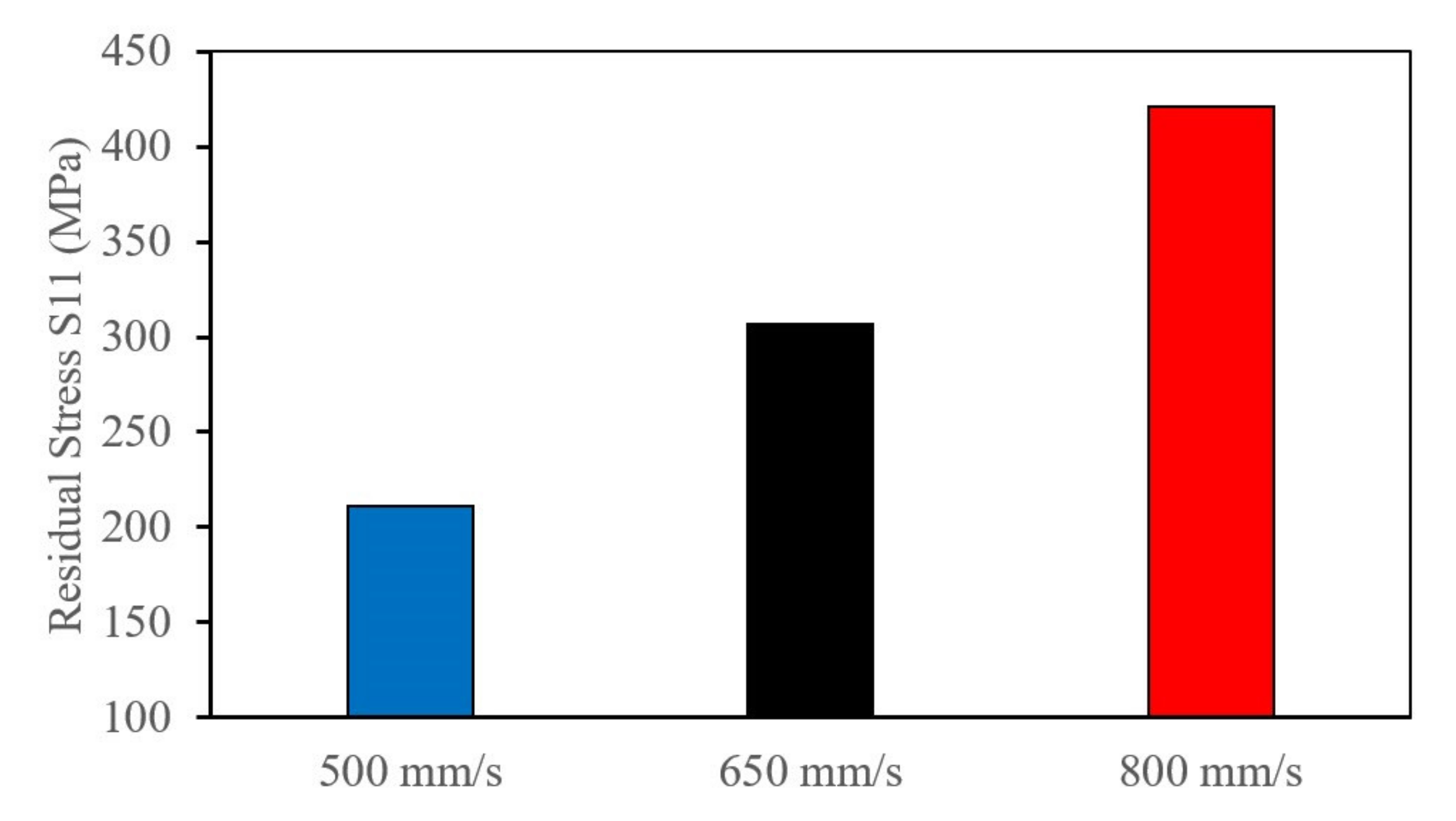
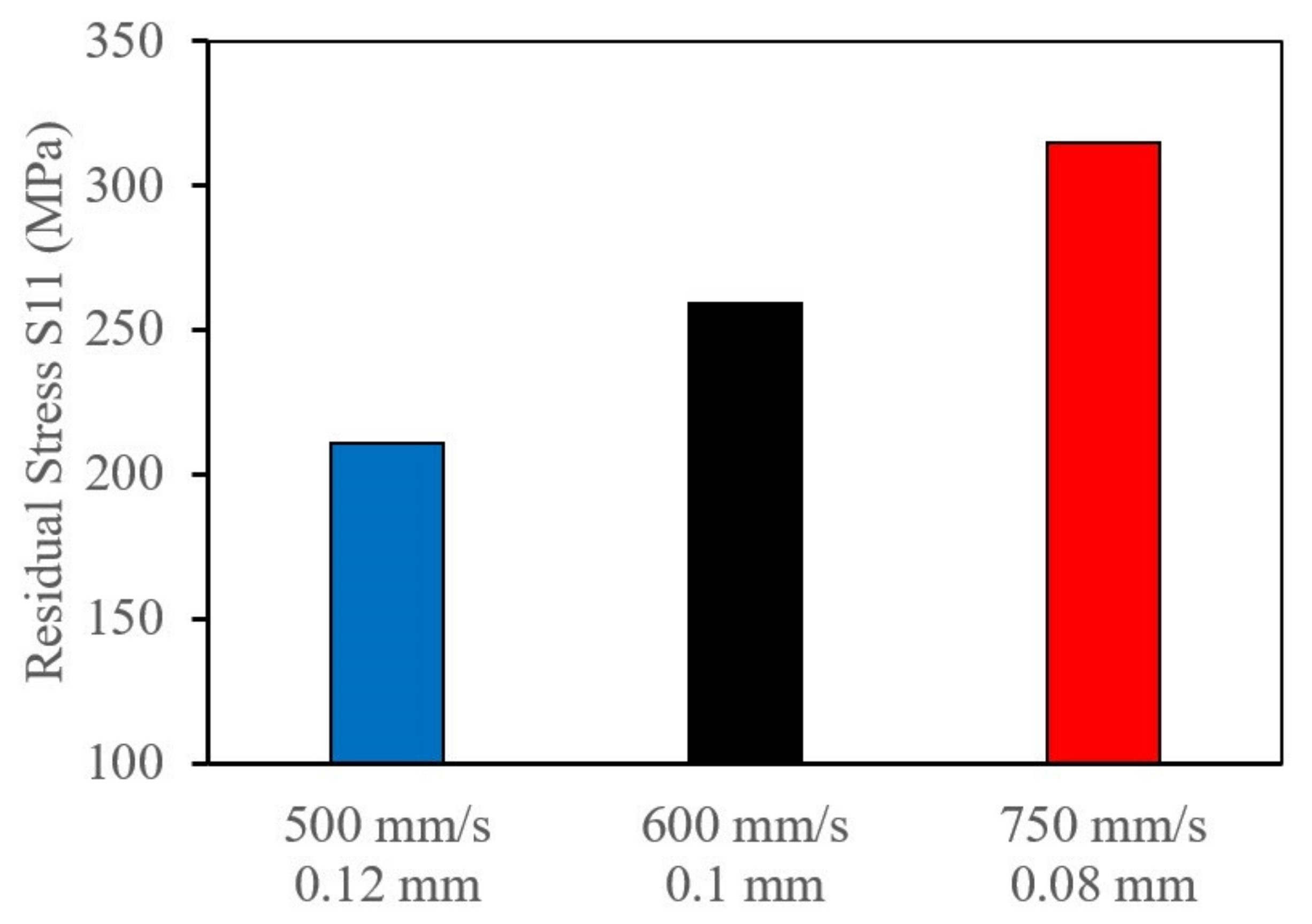
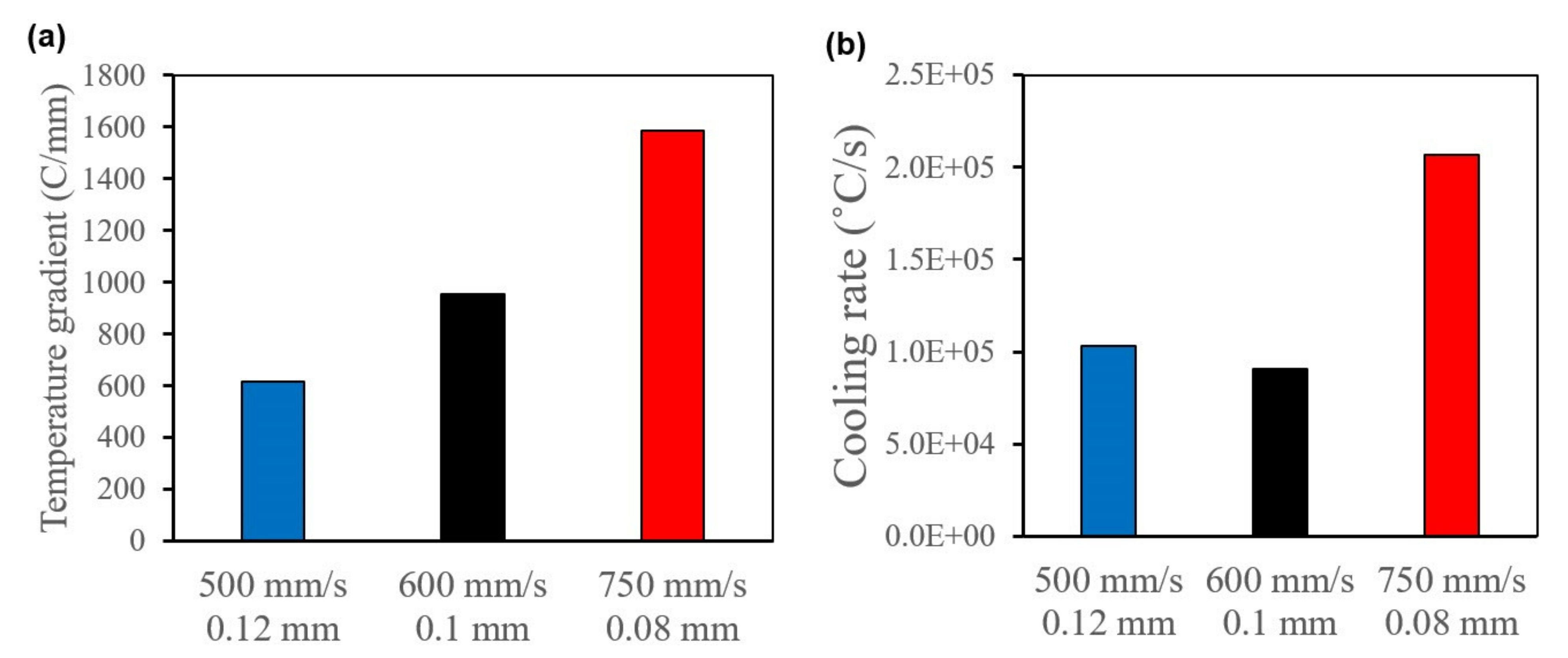
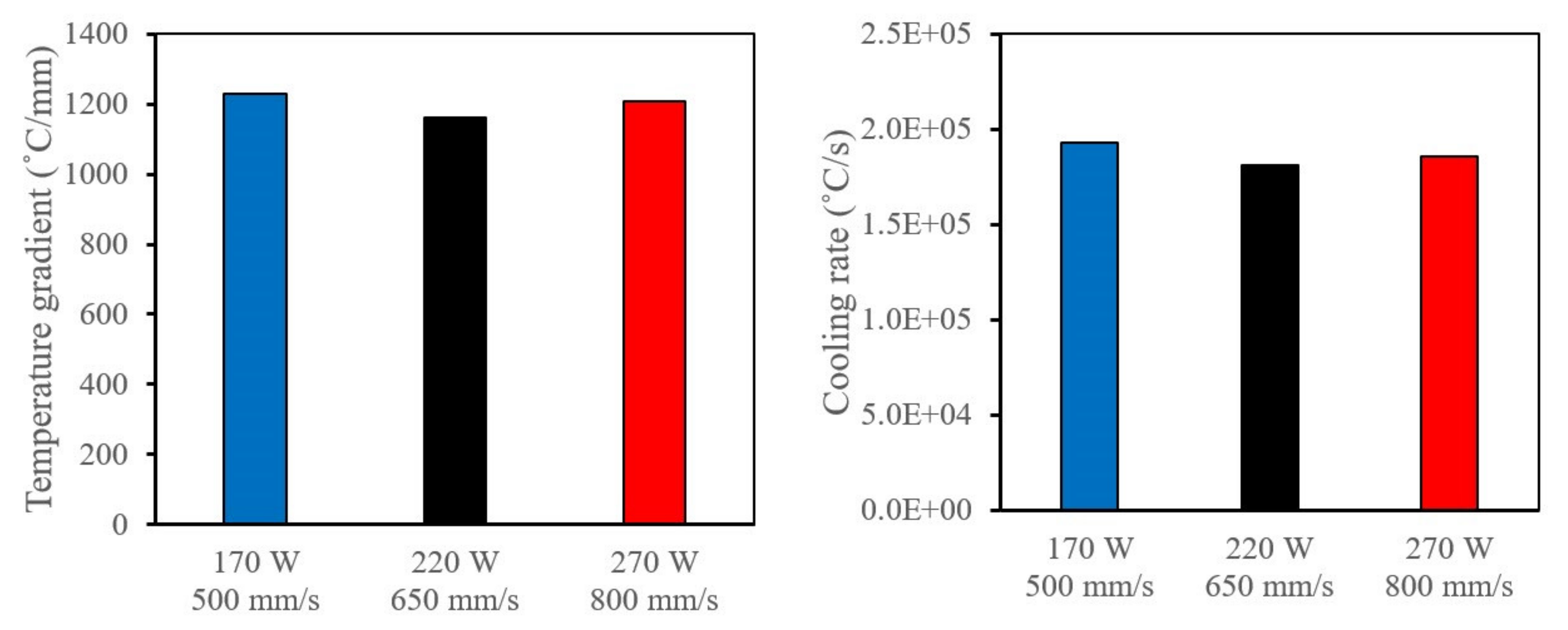
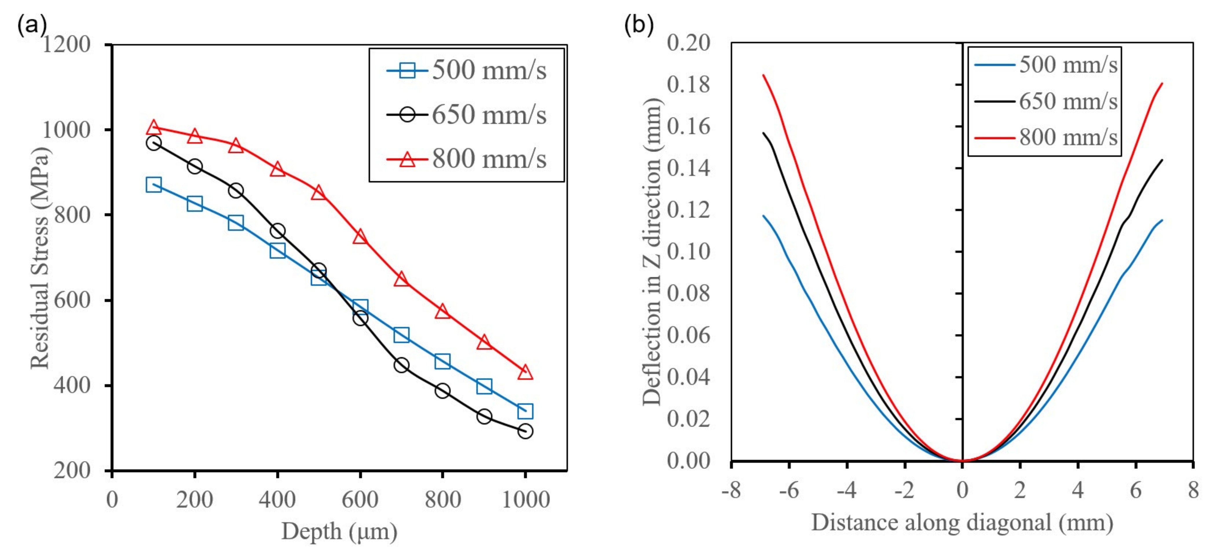
4.2.2. Effect of Scan Speed on RS

Examining the effect of the scan speed on the temperature history at the center point of the layer can be seen in Figure 23, where three scan speed levels of 500 mm/s, 650 mm/s, and 800 mm/s are shown. As expected, the temperature peaks decreased with increasing scan speed. Yet, the temperature at the layer midpoint did not reach the melting temperature during the exposure of track n − 1, as the hatch spacing was greater than the half-width of the melt pool. However, at a scan speed of 500 mm/s, the melt pool half-width was 120 μm, equal to the hatch spacing, but the peak temperature from track n − 1 was just shy of the melting temperature.

Surface RS are measured after laser exposure plus a relaxation time equal to the recoating time of 5 s. It is shown in Figure 24 that tensile RS is formed, and its magnitude increases linearly with the increase in scan speed. The RS increase is due to the corresponding increase in the temperature gradient and CR, Figure 25, which would induce higher thermal stresses. The increase in the temperature gradient occurs even though increasing the scan speed will cause a reduction in the energy density added to the powder layer. The increasing trend can be attributed to the increase in CR, which causes the surrounding material to cool faster, thus creating a more significant temperature difference. In addition, as the speed increases, the melt pool width decreases, resulting in less heating of the adjacent tracks and lower temperature peak, as seen in Figure 23, where the amplitude of the third peak is lower at the higher scan speeds. Therefore, the lower temperatures of the adjacent tracks will lead to a larger temperature gradient.

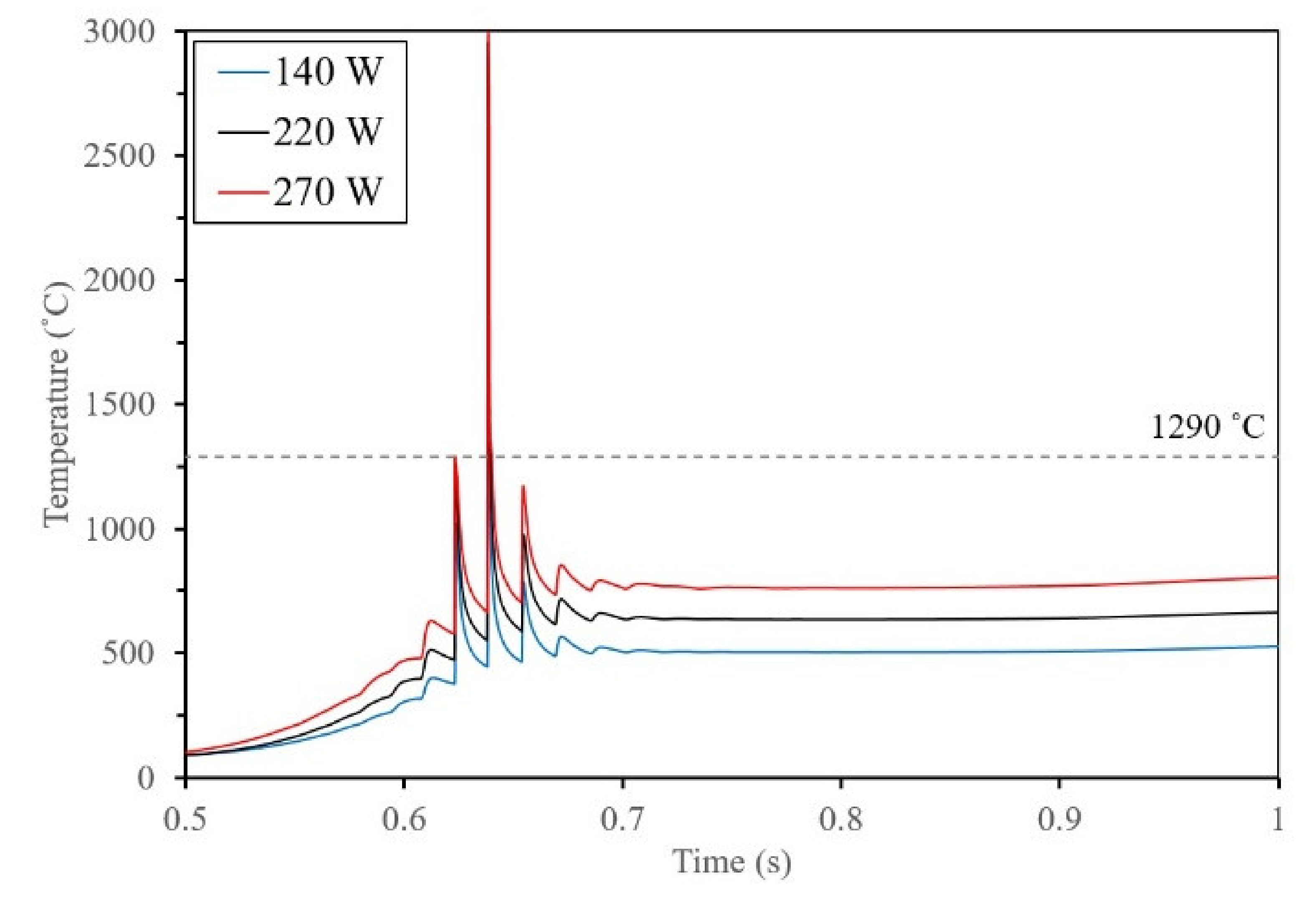
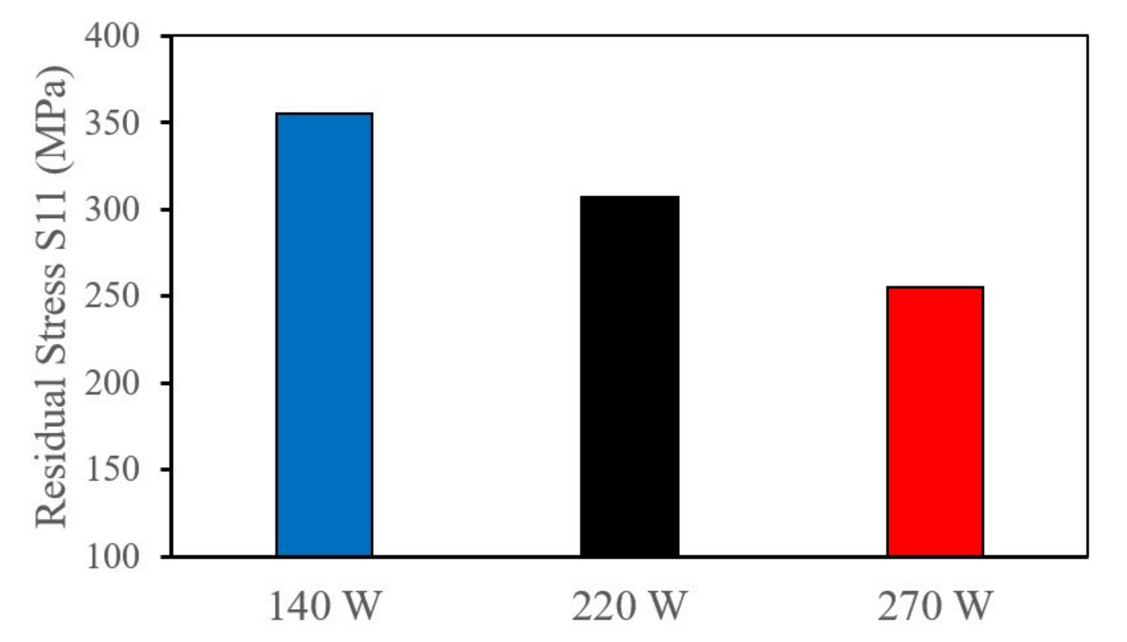
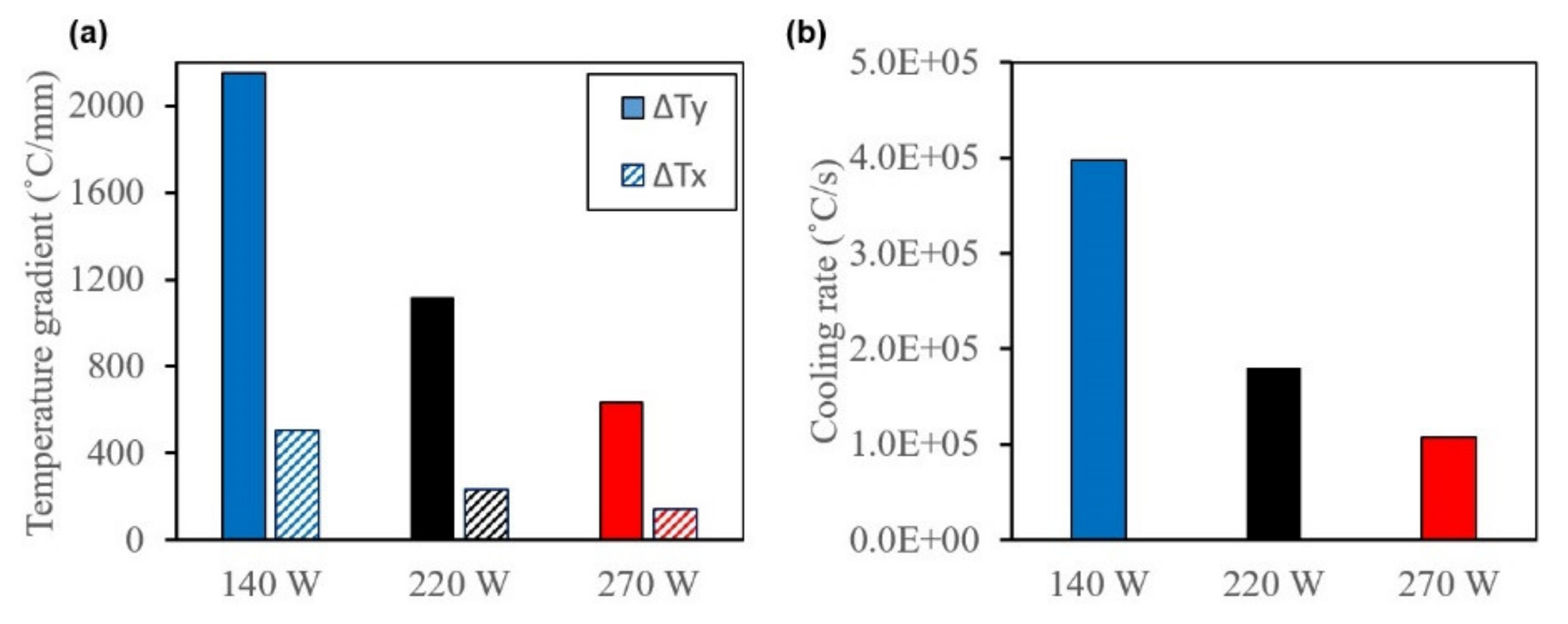
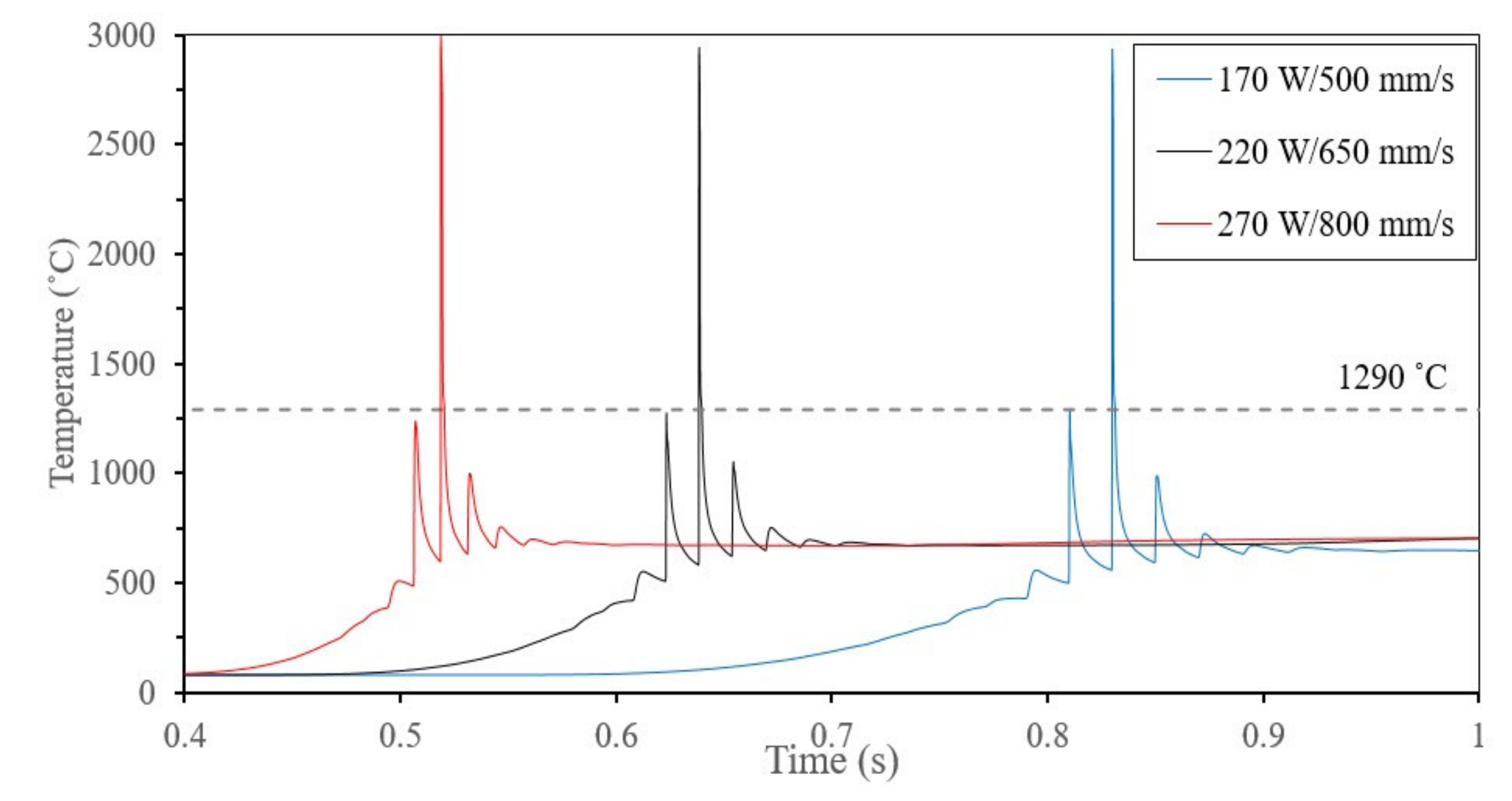
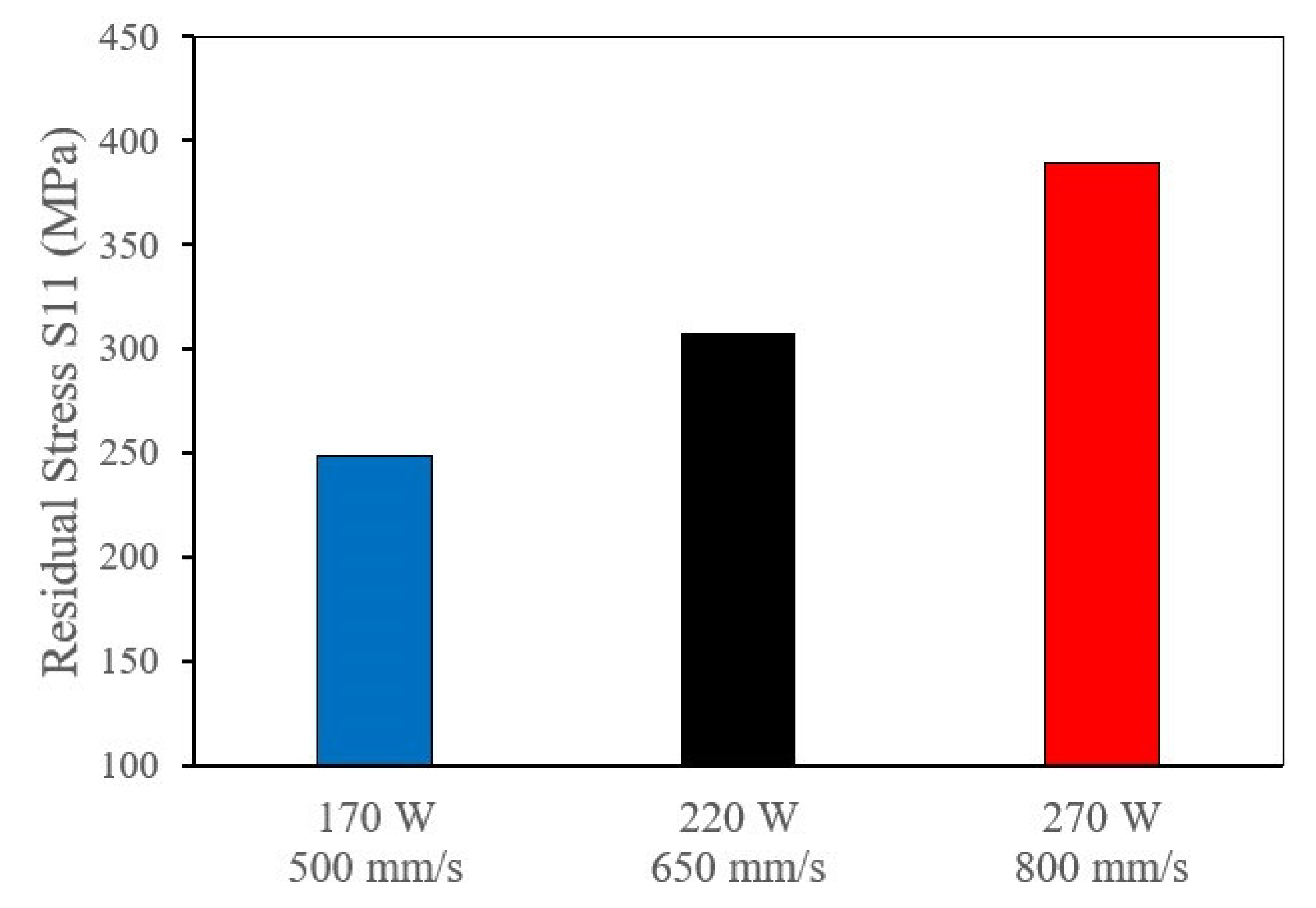
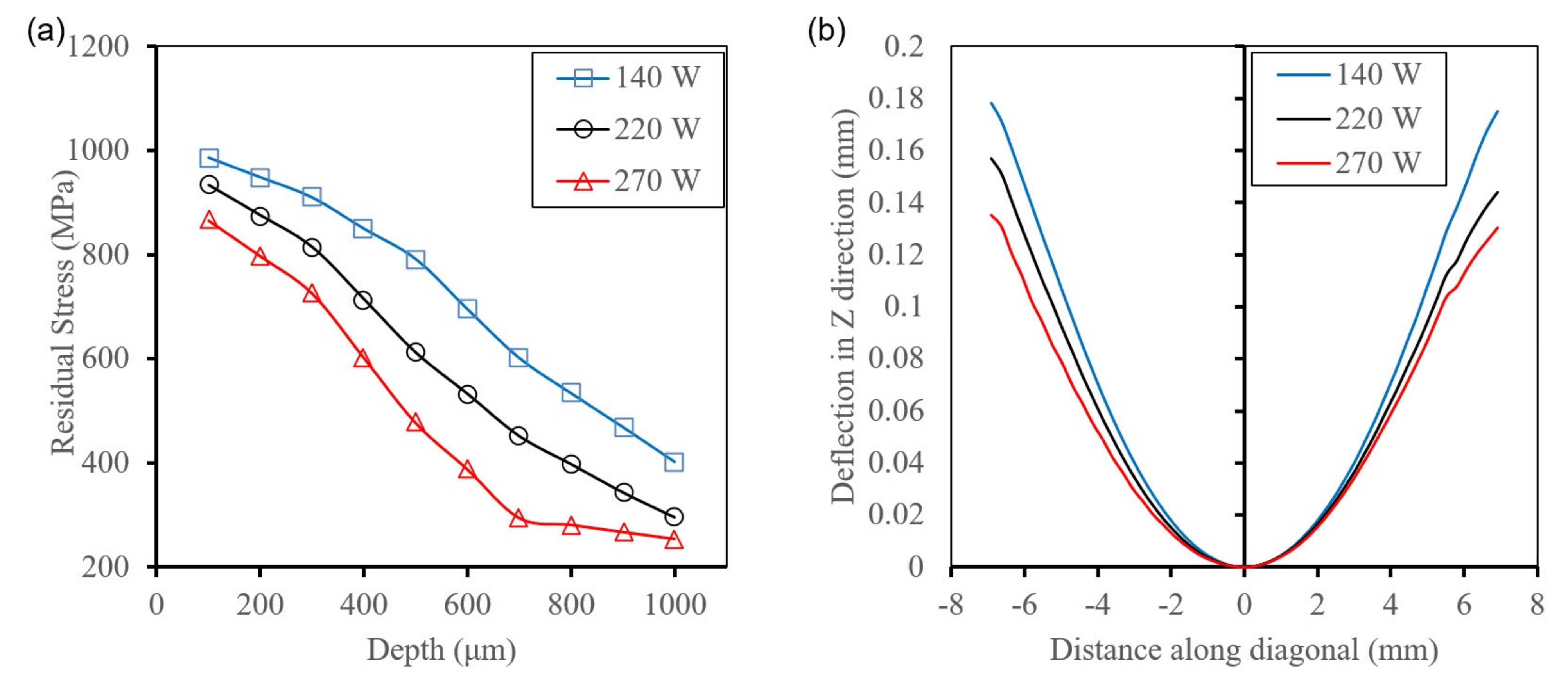
4.2.3. Effect of Laser Power on RS

Three different laser power levels were modeled at a constant scan speed of 650 mm/s and 0.12 mm hatch spacing to examine the effect of laser power on the temperature profiles and RS. The temperature history in Figure 26 shows similar temperature evolutions for all three laser powers at the midpoint of track n. At any time, the minimum temperature is recorded with the 140 W power and increases with increasing the laser power. At 270 W, the melt pool width was 300 μm, which means that the half-width is larger than the hatch spacing. The larger inter-track overlap is reflected in the temperature history profile, where the point on track n reached the melting point while the laser was still scanning track n − 1, seen as the first peak on the red curve in Figure 26.

Prediction of RS at the midpoint of track n shows that a laser power of 140 W resulted in the highest surface RS, as shown in Figure 27, and RS decreases with the increase in laser power, which agrees with the literature [50]. The declining trend in RS is analogous to the temperature gradient and CR trend, shown in Figure 28, where the highest temperature gradient is recorded at 140 W. The decreasing trend can be traced back to the melt pool size, where the widths are measured to be 138 μm, 176 μm, and 298 μm, corresponding to 140 W, 220 W, and 270 W, respectively. Therefore, the wider melt pool will have a larger heat-affected zone (HAZ), as shown in Figure 29, and the surrounding material will have a higher temperature. The higher temperature of the HAZ is evident by the amplitude of the third peak in Figure 26, which increases with the increase in laser power. The higher the amplitude, the lower the temperature difference between the second (below solidus temperature) and third peak, corresponding to a lower temperature gradient.

4.2.4. Effect of Hatch Spacing on RS

The increase in hatch spacing from 0.08 mm to 0.12 mm resulted in a temperature history profile, Figure 30, different from that under varying scan speed or laser power. At 0.08 mm, the distance between subsequent tracks is small, so that the temperature of track n has peaked above the melting temperature three distinct times by the first three peaks on the blue curve in Figure 30. As the hatch spacing increases to 0.1, there are only two peaks above the melting point. At the largest hatch spacing, there is not enough heat conducted between tracks to raise the temperature of track n, thus leading to only one peak above the melting point.

The increase in hatch spacing, i.e., the decrease in energy density, caused the surface RS to drop from 389 MPa to 307 MPa, as shown in Figure 31. Conversely, the decrease in energy density by increasing the scan speed or decreasing the laser power led to an increase in surface RS, as shown in Figure 24 and Figure 27.

It is found that the surface RS trend is governed by the temperature gradient, which had a more dominant effect on the surface RS than the CR, as shown in Figure 32. As the hatch spacing increases from 0.08 mm to 0.1 mm, the temperature gradient decreases; hence, the surface RS decrease. However, increasing the hatch spacing from 0.1 mm to 0.12 caused a reduction in the temperature gradient and an opposite increase in the CR, leading to a slightly lower surface RS.

4.2.5. Effect of Same Energy Density

Studying the effects of laser power, scan speed, and hatch spacing on surface RS shows opposing effects and, consequently, non-monotonic trends for the effect of the energy density on the surface RS. Therefore, the effect of the individual process parameters needs to be investigated at constant energy density. The first set of simulations are performed at an energy density of 3.67 $\mathrm{J}\mathrm{/}\mathrm{m}{\mathrm{m}}^2$ with a constant laser power of 220 W. Three levels for the scan speed, 500 mm/s, 600 mm/s, and 750 mm/s, and three hatch spacings, 0.12 mm, 0.1 mm, and 0.08 mm, are selected, respectively.

The temperature history, presented in Figure 33, shows that all three parameter combinations resulted in multiple temperatures peaks above the melting point. However, it is noticed that the maximum peak temperature was achieved at the lowest scan speed of 500 mm/s and the largest hatch spacing, which means that the scan speed has a more dominant effect on the maximum temperature versus the hatch spacing. Conversely, the hatch spacing has a more dominant effect when it comes to raising the temperature of the adjacent tracks, where the least hatch spacing resulted in two subsequent peaks with peak temperature highly above the melting point, as seen by the red curve in Figure 33.

Examining the effect of the distinct temperature histories on the surface RS, presented in Figure 34, shows that the surface RS are lowest at 500 mm/s and 0.12 mm with a magnitude of 211 MPa and increase non-linearly to reach a maximum value of 454 MPa at 750 mm/s and 0.08 mm.

The non-linear trend in the temperature gradient, shown in Figure 35, is the driver of the surface RS as the temperature gradient increases with the increase in scan speed and decrease in the hatch spacing. However, the CR decreases when the scan speed increases from 500 mm/s to 600 mm/s then increases beyond that point, which means that the temperature gradient mainly affects the surface RS. It can also be deduced that the scan speed has a more dominant effect than the hatch spacing on the surface RS, since increasing the hatch spacing from 0.1 mm to 0.12 resulted in a negligible change in the surface RS, as shown in Figure 31. However, the variation of the scan speed caused the surface RS to increase significantly.

To further investigate the effect of process parameters on surface RS with the same energy density, the laser power and scan speed are varied, while the hatch spacing is kept constant at 0.12 mm. Three power levels, 170 W, 220 W, and 270 W, and three scan speeds, 500 mm/s, 650 mm/s, and 800 mm/s, gave an energy density of 2.82 $\mathrm{J}\mathrm{/}\mathrm{m}{\mathrm{m}}^2$. All three parameter combinations resulted in almost identical temperature profiles, with a slight difference in the magnitude of the peaks, as shown in Figure 36.

The results presented in Section 4.2.2 and Section 4.2.3 show that the increase in scan speed caused an increase in surface RS; conversely, the increase in laser power caused a decrease in surface RS. However, the combined effect of increasing the laser power and scan speed increased surface RS, as shown in Figure 37. Therefore, the scan speed has a more dominant effect on the surface RS than the laser power. To investigate the underlying causes that drive this trend in the surface RS, the temperature gradients and CRs are plotted in Figure 38.

The highest temperature gradient and CR were recorded at the lowest laser power and scan speed. Increasing the laser power and scan speed causes the temperature gradient and CR to decrease slightly and increase as the laser power and scan speed increase. Based on the previous observations, the surface RS followed the same trend as the temperature gradient. Therefore, if applied here, the surface RS should have been the highest at the 170 W/ 500 mm/s combination, decreasing at 220 W/650 mm/s, and then increasing again at 270 W/800 mm/s. However, this is not the case, as shown in Figure 37. Therefore, an in-depth investigation of the temperature and stress history is required.

The temperature and stress evolutions, plotted in Figure 39, show that, after the laser melts track n, the material starts to solidify and generates high thermal stresses. The stress reaches a magnitude of 460 MPa, 440 MPa, and 445 MPa, corresponding to 170 W/500 mm/s, 220 W/650 mm/s, and 270 W/800 mm/s, respectively. The trend of these stresses is similar to the temperature gradients shown in Figure 38. However, the final stress state is not reached yet, and further stress changes occur with the subsequent laser passes. As heat is conducted from the subsequent tracks, the temperature of track n rises, thus relieving the previously generated stresses causing the cyclic change in stresses shown in the left column in Figure 39. As the laser travels far enough from track n, the magnitude of the cyclic stress decreases. The conducted heat will keep reaching track n until the laser has finished scanning the whole layer; hence, the more time it takes for the laser to scan the layer, the more heat is conducted and, consequently, the greater the reduction in the stress magnitude. The laser scanning time from track n to the end of the layer is calculated at 0.84 s, 0.6 s, and 0.52 s, corresponding to 500 mm/s, 650 mm/s, and 800 mm/s, respectively, as shown in the right column of Figure 39. The difference in time durations allows the conducted heat to reduce the stresses to −80 MPa, −21 MPa, and 70 MPa, respectively. Once the laser finishes scanning, the temperature of the whole layer cools down for the same period, thus raising the stresses to their final state, where the lowest stress is recorded at 170 W and 500 mm/s.

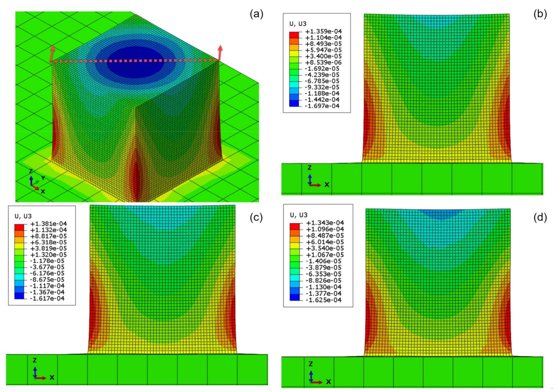
4.3. Part Scale Model

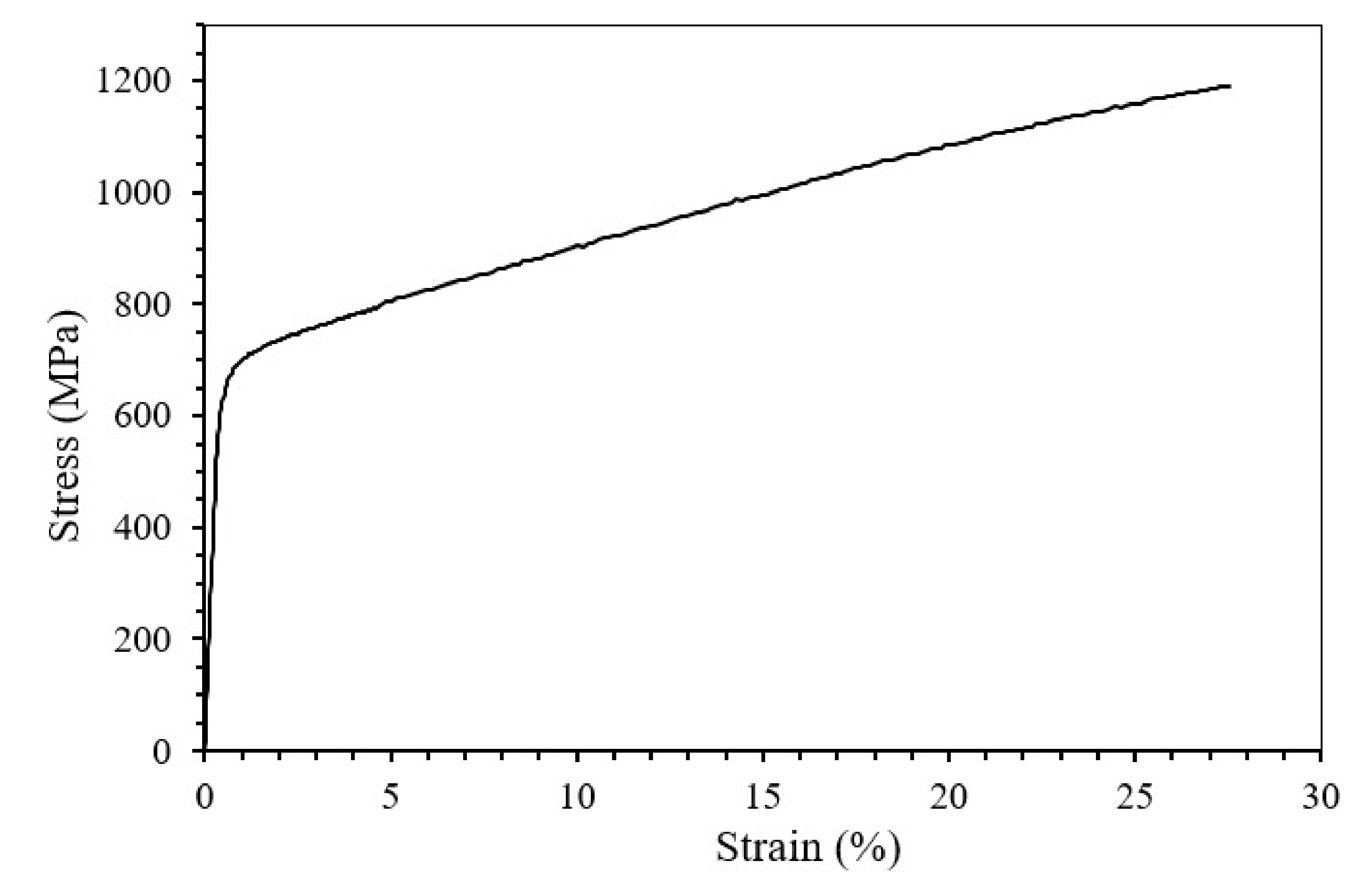
4.3.1. Tensile Test

Tensile testing of as-built condition showcased the sample undergoing ductile failure as presented by the true stress–strain curve shown in Figure 40. The yield strength at 0.2% elongation was 650 MPa, with a Young’s modulus of 171 GPa, and the ultimate strength was 1191 MPa. By fitting the data to the Ramberg–Osgood equation, the strength coefficient was found to be 1618 MPa, and the strain hardening exponent was 0.243.

The J–C model’s A, B, and n parameters were changed to the new value to compare the predicted RS in-depth profile with the experimental data. Due to the absence of tensile testing data for different process parameters, the same values of A, B, and n were used for all simulated process parameters. Additionally, since the measured Young’s modulus is lower than its values reported in the literature, the newly measured value was used in the current study. Finally, Young’s modulus was measured at room temperature. Still, Young’s modulus data from the literature were offset by the difference between measured to obtain its values at high temperature. Their reported values were obtained at room temperature, as shown in Figure 41.

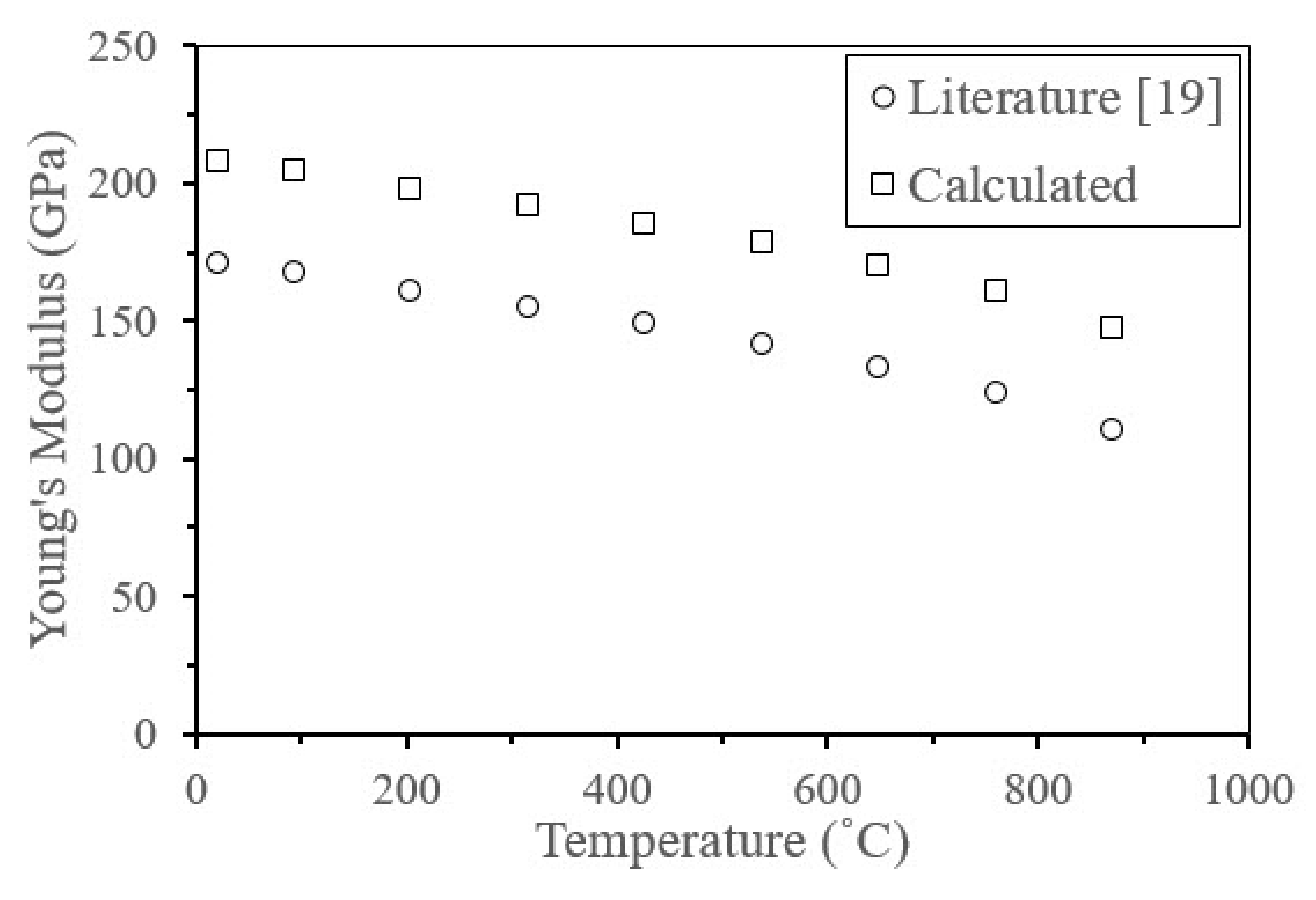
4.3.2. Numerical Results

The part scale model is used to predict the RS distribution across the whole part and the deflection of the part, which will affect its dimensional accuracy. The evolution of the Mises stress can be seen in Figure 42 at different time instances. At a time of 667 s, i.e., after a 4 mm height (Figure 42a), the maximum stresses are predicted at the bottom of the part, at the interface between the part and the substrate. As the number of layers increases to reach 10 mm, more heat is added to the top surface of the part and conducts downwards, causing the stress magnitude to decrease, as shown in Figure 42b. Once the laser exposure is completed, the part begins to cool down for 600 s, at which point the stresses in the part increase again (Figure 42c) to reach its maximum value. Once the part is separated from the substrate, the stress magnitudes decrease to reach their final value, as shown in Figure 42d.

The RS were calculated at the end of the building process after a cooling time of 600 s and separation from the build plate. The RS were calculated by averaging the stresses across an area with a diameter of 2 mm. The predicted in-depth RS profile is validated by comparing to experimentally measured RS profile at two laser powers, 220 W and 140 W, a scan speed of 650 mm/s, and a hatch spacing of 0.12 mm, as shown in Figure 43 and Figure 44, respectively.

Two RS profiles are compared to the experimental results: the first RS profile is calculated using the J–C parameters found in the literature [65]. The second RS profile is predicted with J–C parameters partially adjusted using data from tensile testing of IN625 manufactured using LPBF. It is found that the first profile under predicts the in-depth RS, while the second profile over predicts the RS profile. However, both profiles follow the same trend as the experimental results. These results highlight the need for J–C plasticity parameters for LPBF-manufactured IN625 to predict the generated stresses better.

Prediction of the in-depth RS with increasing the hatch spacing shows that the hatch spacing does not affect the RS profile, as shown in Figure 45, regardless of the laser power used. The hatch effect absence could be attributed to using a point source heat model, which does not generate the teardrop shape of a melt pool, so the effect of melt pool overlap is negated and would not affect the predicted RS.

Examining the effect of laser power on the in-depth RS and deflection show that increasing the laser power from 140 W to 270 W decreases the in-depth RS, as seen in Figure 46. However, the generated RS for all three laser powers are highly tensile down to a depth of 1 mm from the surface. This trend is similar to that predicted from the layer model for the surface RS, as presented in Section 4.2.3. Increasing the scan speed also showed a similar trend to the results reported in Section 4.2.2. The in-depth RS increased with increasing the scan speed, as shown in Figure 47a.

The deflection of the top surface in the Z direction is of particular interest, as it increases the chances of the recoater impacting the part and damaging or breaking the part off. Therefore, the deflection was extracted along the diagonal of the part, as shown in Figure 48a. It is observed that after cutting the part from the build plate, the edges of the part deflect upwards. At the same time, the center sinks in, resulting in a parabola-shaped surface.

Examining the effect of process parameters on the deflection shows that the laser power has the same effect on the deflection as on RS, as seen in Figure 46b, where the lowest power resulted in the largest deflection. Conversely, the scan speed increased top surface deflection, as shown in Figure 47b. This is because the deflection of the part edges means that part of the generated stresses is released; hence, the magnitude of the stresses is always lower at the outer edges.

5. Conclusions

The current work presented a systematic approach to different modeling scales of laser powder bed fusion of IN625, including single tracks, multi-tracks, and multi-layer models. The shortcomings found in the literature were addressed by employing a Gaussian volumetric heat source model, a material model to accurately represent the thermos-physical properties of the powder layer, artificial inclusion of the Marangoni effect, and the use of the Johnson–Cook plasticity model to include the strain hardening, strain rate effect, and thermal softening of the material. The results from all models were validated with multiple experimental results, including melt pool dimensions, temperature measurements using a two-color pyrometer, and in-depth residual stress profiles. The main findings can be summarized as follows:

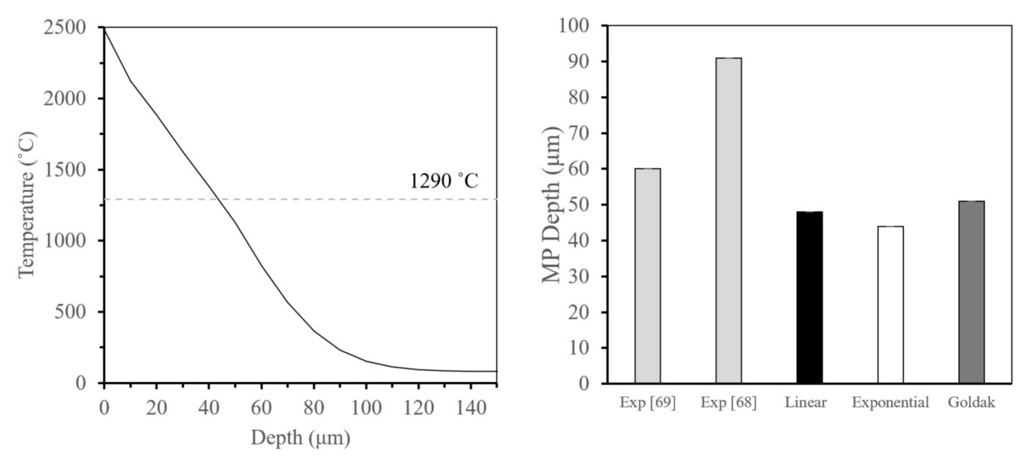
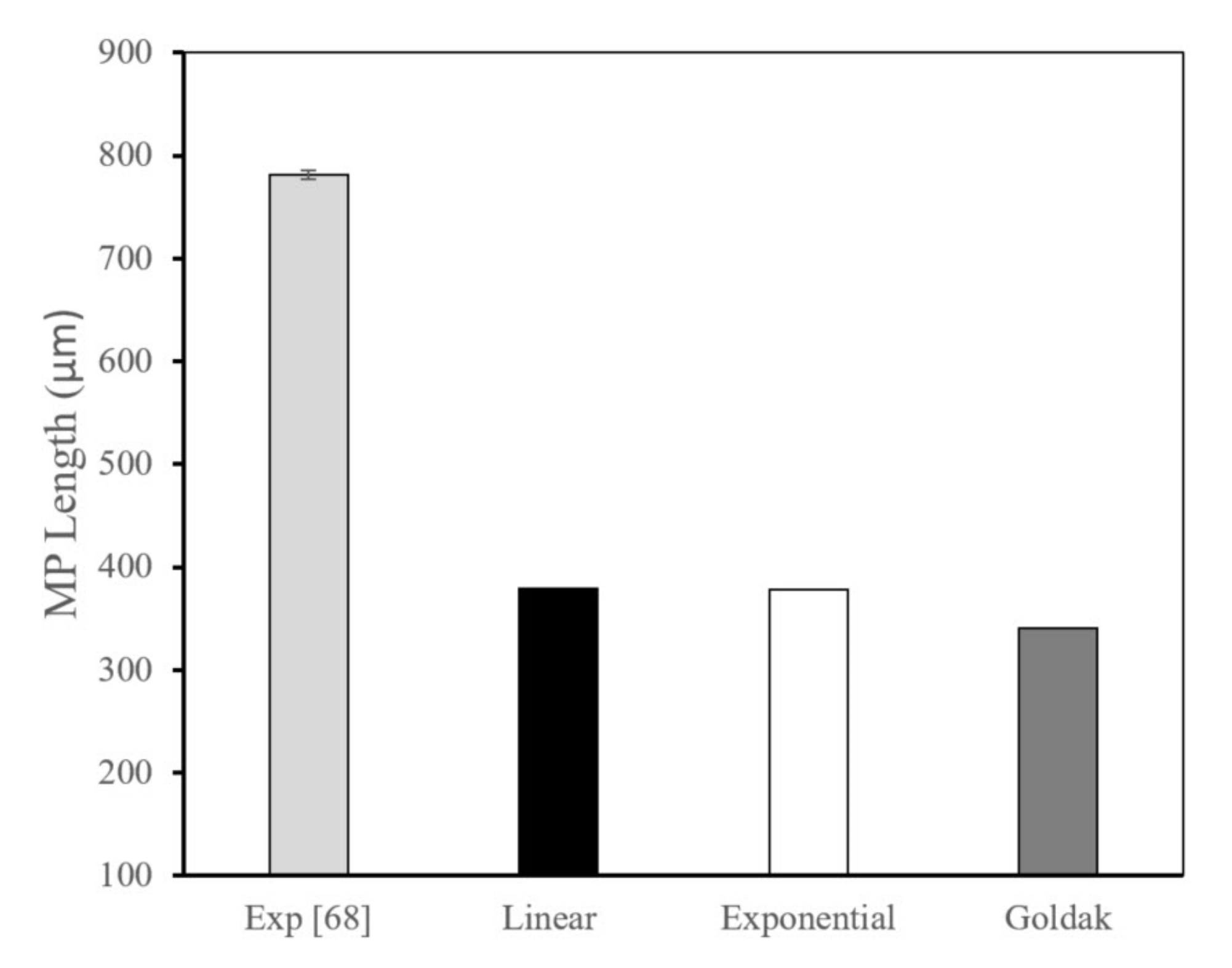
• The exponential decay volumetric heat source, with an artificial increase in thermal conductivity to account for the Marangoni effects, resulted in the best prediction of melt pool dimensions.
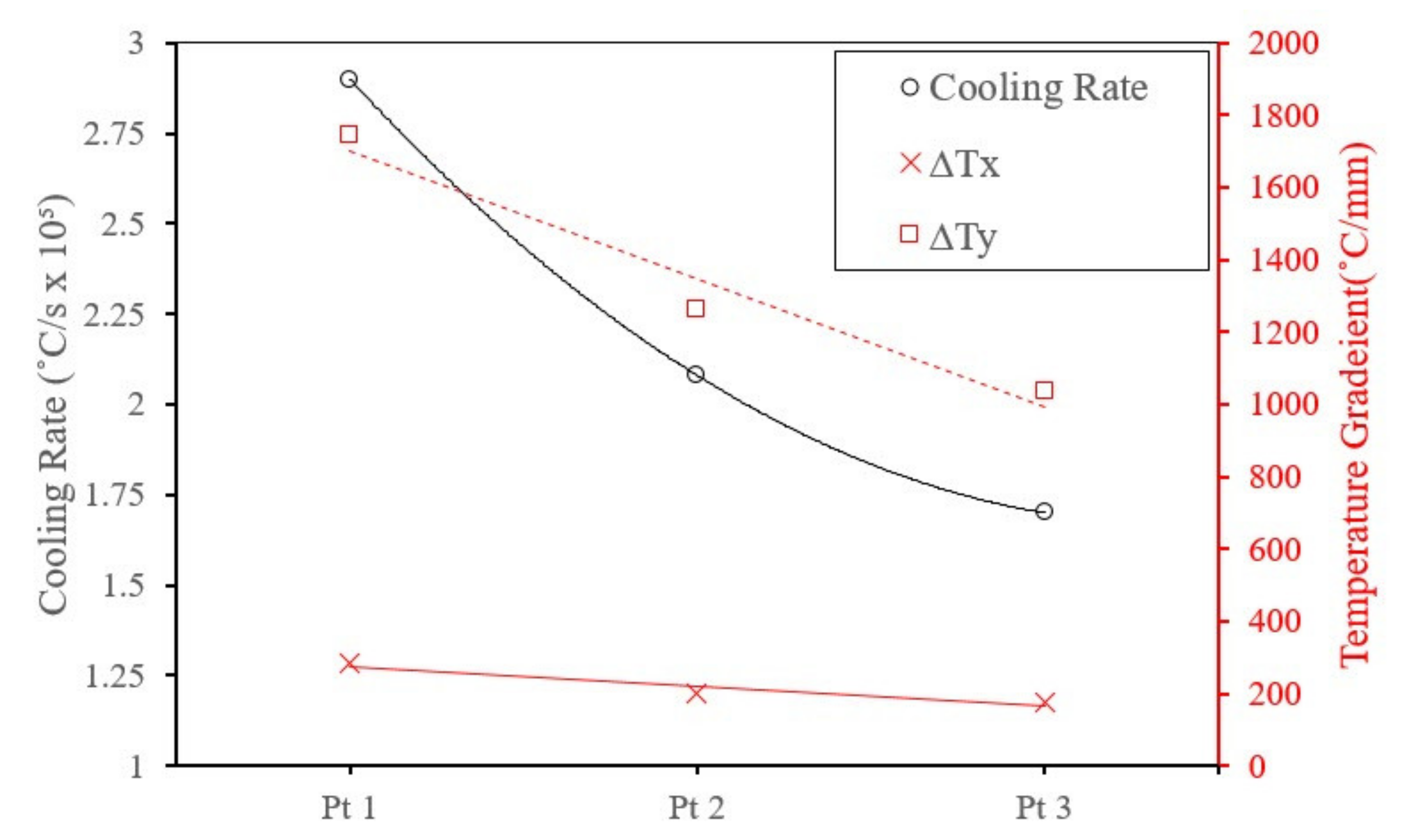
• The maximum residual stress is generated along the laser scan direction, governed by the temperature gradient and cooling rate in the hatch direction.
• Increasing the scan speed resulted in an increase in the surface tensile residual stress due to the increase in the temperature gradient.
• The surface tensile residual stress decreases with the increase in hatch spacing.
• At the same energy density, the thermal stresses are mostly affected by the scan speed, laser power, and hatch spacing.
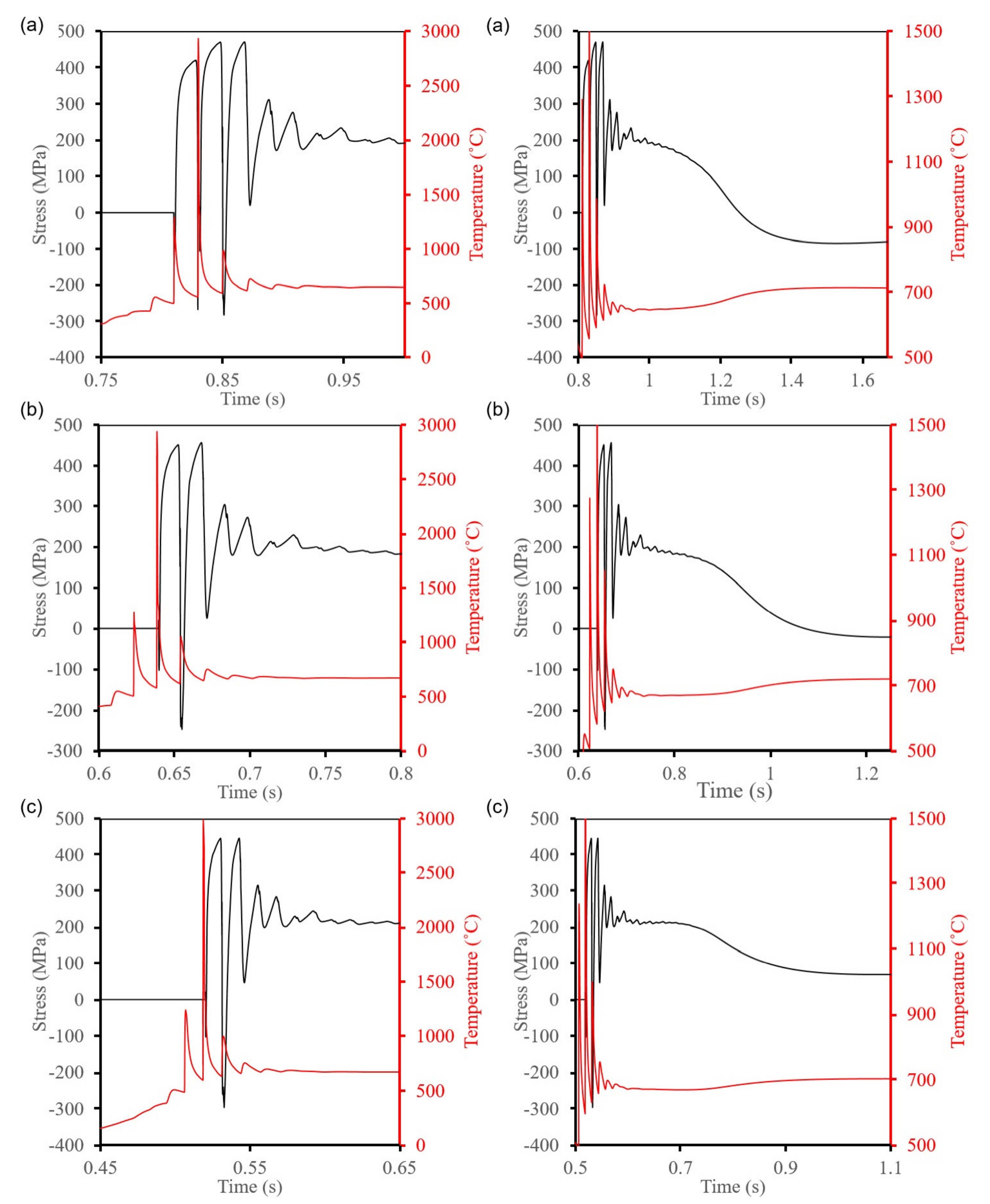
• Although the high cooling rate will increase the strain rate experienced by the material, the evolution of the stresses is mainly dominated by the temperature gradient.
• The cyclic temperature governs the final state of the stress during the non-linear phase and the cooling rate during the linear phase.
• In-depth residual stresses on a part scale and the top surface deflection exhibit the same trend, where increasing the laser power lowers the residual stresses.
• Increasing the scan speed increases the in-depth residual stresses as well as the top surface deflection.

References

- ISO/ASTM52900-15, Standard Terminology for Additive Manufacturing—General Principles—Terminology; ASTM International: West Conshohocken, PA, USA. 2015. Available online: www.astm.org (accessed on 1 September 2021).
- DebRoy, T.; Wei, H.; Zuback, J.; Mukherjee, T.; Elmer, J.; Milewski, J.; Beese, A.M.; Wilson-Heid, A.D.; De, A.; Zhang, W. Additive manufacturing of metallic components—Process, structure and properties. Prog. Mater. Sci. 2018, 92, 112–224. [Google Scholar] [CrossRef]
- Armillotta, A.; Baraggi, R.; Fasoli, S. SLM tooling for die casting with conformal cooling channels. Int. J. Adv. Manuf. Technol. 2014, 71, 573–583. [Google Scholar] [CrossRef] [Green Version]
- Dehoff, R.; Duty, C.; Peter, W.; Yamamoto, Y.; Chen, W.; Blue, C.; Tallman, C. Case study: Additive manufacturing of aerospace brackets. Adv. Mater. Process. 2013, 171, 19–23. [Google Scholar]
- Huang, R.; Riddle, M.; Graziano, D.; Warren, J.; Das, S.; Nimbalkar, S.; Cresko, J.; Masanet, E. Energy and emissions saving potential of additive manufacturing: The case of lightweight aircraft components. J. Clean. Prod. 2016, 135, 1559–1570. [Google Scholar] [CrossRef] [Green Version]
- Leal, R.; Barreiros, F.; Alves, L.; Romeiro, F.; Vasco, J.; Santos, M.; Marto, C. Additive manufacturing tooling for the automotive industry. Int. J. Adv. Manuf. Technol. 2017, 92, 1671–1676. [Google Scholar] [CrossRef]
- Zhang, B.; Li, Y.; Bai, Q. Defect formation mechanisms in selective laser melting: A review. Chin. J. Mech. Eng. 2017, 30, 515–527. [Google Scholar] [CrossRef] [Green Version]
- Piscopo, G.; Salmi, A.; Atzeni, E. On the quality of unsupported overhangs produced by laser powder bed fusion. Int. J. Manuf. Res. 2019, 14, 198–216. [Google Scholar] [CrossRef] [Green Version]
- Balbaa, M.; Ghasemi, A.; Fereiduni, E.; Elbestawi, M.; Jadhav, S.; Kruth, J.-P. Role of powder particle size on laser powder bed fusion processability of AlSi10Mg alloy. Addit. Manuf. 2020, 37, 101630. [Google Scholar] [CrossRef]
- Criales, L.E.; Arısoy, Y.M.; Lane, B.; Moylan, S.; Donmez, A.; Özel, T. Laser powder bed fusion of nickel alloy 625: Experimental investigations of effects of process parameters on melt pool size and shape with spatter analysis. Int. J. Mach. Tools Manuf. 2017, 121, 22–36. [Google Scholar] [CrossRef]
- Maamoun, A.H.; Xue, Y.F.; Elbestawi, M.A.; Veldhuis, S.C. Effect of selective laser melting process parameters on the quality of al alloy parts: Powder characterization, density, surface roughness, and dimensional accuracy. Materials 2018, 11, 2343. [Google Scholar] [CrossRef] [Green Version]
- Narvan, M.; Al-Rubaie, K.S.; Elbestawi, M. Process-structure-property relationships of AISI H13 tool steel processed with selective laser melting. Materials 2019, 12, 2284. [Google Scholar] [CrossRef] [Green Version]
- Sealy, M.P.; Madireddy, G.; Williams, R.E.; Rao, P.; Toursangsaraki, M. Hybrid processes in additive manufacturing. J. Manuf. Sci. Eng. 2018, 140, 060801. [Google Scholar] [CrossRef]
- Han, S.; Salvatore, F.; Rech, J.; Bajolet, J. Abrasive flow machining (AFM) finishing of conformal cooling channels created by selective laser melting (SLM). Precis. Eng. 2020, 64, 20–33. [Google Scholar] [CrossRef]
- Kruth, J.-P.; Deckers, J.; Yasa, E.; Wauthlé, R. Assessing and comparing influencing factors of residual stresses in selective laser melting using a novel analysis method. Proc. Inst. Mech. Eng. Part B J. Eng. Manuf. 2012, 226, 980–991. [Google Scholar] [CrossRef]
- Narvan, M.; Ghasemi, A.; Fereiduni, E.; Kendrish, S.; Elbestawi, M. Part deflection and residual stresses in laser powder bed fusion of H13 tool steel. Mater. Des. 2021, 204, 109659. [Google Scholar] [CrossRef]
- Yang, Y.; Allen, M.; London, T.; Oancea, V. Residual strain predictions for a powder bed fusion Inconel 625 single cantilever part. Integr. Mater. Manuf. Innov. 2019, 8, 294–304. [Google Scholar] [CrossRef] [Green Version]
- Simson, T.; Emmel, A.; Dwars, A.; Böhm, J. Residual stress measurements on AISI 316L samples manufactured by selective laser melting. Addit. Manuf. 2017, 17, 183–189. [Google Scholar] [CrossRef]
- Kruth, J.-P.; Mercelis, P.; Van Vaerenbergh, J.; Froyen, L.; Rombouts, M. Binding mechanisms in selective laser sintering and selective laser melting. Rapid Prototyp. J. 2005, 11, 26–36. [Google Scholar] [CrossRef] [Green Version]
- Hussein, A.; Hao, L.; Yan, C.; Everson, R. Finite element simulation of the temperature and stress fields in single layers built without-support in selective laser melting. Mater. Des. 2013, 52, 638–647. [Google Scholar] [CrossRef]
- Fu, C.; Guo, Y. 3-dimensional finite element modeling of selective laser melting Ti-6Al-4V alloy. In Proceedings of the 25th Annual International Solid Freeform Fabrication Symposium, Austin, TX, USA, 4–6 August 2014. [Google Scholar]
- Roberts, I.; Wang, C.; Esterlein, R.; Stanford, M.; Mynors, D. A three-dimensional finite element analysis of the temperature field during laser melting of metal powders in additive layer manufacturing. Int. J. Mach. Tools Manuf. 2009, 49, 916–923. [Google Scholar] [CrossRef]
- Dong, L.; Makradi, A.; Ahzi, S.; Remond, Y. Three-dimensional transient finite element analysis of the selective laser sintering process. J. Mater. Process. Technol. 2009, 209, 700–706. [Google Scholar] [CrossRef]
- Dong, L.; Correia, J.; Barth, N.; Ahzi, S. Finite element simulations of temperature distribution and of densification of a titanium powder during metal laser sintering. Addit. Manuf. 2017, 13, 37–48. [Google Scholar] [CrossRef]
- Andreotta, R.; Ladani, L.; Brindley, W. Finite element simulation of laser additive melting and solidification of Inconel 718 with experimentally tested thermal properties. Finite Elem. Anal. Des. 2017, 135, 36–43. [Google Scholar] [CrossRef]
- Khairallah, S.A.; Anderson, A. Mesoscopic simulation model of selective laser melting of stainless steel powder. J. Mater. Process. Technol. 2014, 214, 2627–2636. [Google Scholar] [CrossRef]
- Mukherjee, T.; Wei, H.; De, A.; DebRoy, T. Heat and fluid flow in additive manufacturing—Part I: Modeling of powder bed fusion. Comput. Mater. Sci. 2018, 150, 304–313. [Google Scholar] [CrossRef] [Green Version]
- Robichaud, J.; Vincent, T.; Schultheis, B.; Chaudhary, A. Integrated computational materials engineering to predict melt-pool dimensions and 3D grain structures for selective laser melting of Inconel 625. Integr. Mater. Manuf. Innov. 2019, 8, 305–317. [Google Scholar] [CrossRef]
- Xia, M.; Gu, D.; Yu, G.; Dai, D.; Chen, H.; Shi, Q. Influence of hatch spacing on heat and mass transfer, thermodynamics and laser processability during additive manufacturing of Inconel 718 alloy. Int. J. Mach. Tools Manuf. 2016, 109, 147–157. [Google Scholar] [CrossRef]
- Denlinger, E.R.; Jagdale, V.; Srinivasan, G.; El-Wardany, T.; Michaleris, P. Thermal modeling of Inconel 718 processed with powder bed fusion and experimental validation using in situ measurements. Addit. Manuf. 2016, 11, 7–15. [Google Scholar] [CrossRef]
- Criales, L.E.; Arısoy, Y.M.; Lane, B.; Moylan, S.; Donmez, A.; Özel, T. Predictive modeling and optimization of multi-track processing for laser powder bed fusion of nickel alloy 625. Addit. Manuf. 2017, 13, 14–36. [Google Scholar] [CrossRef]
- Masoomi, M.; Thompson, S.M.; Shamsaei, N. Laser powder bed fusion of Ti-6Al-4V parts: Thermal modeling and mechanical implications. Int. J. Mach. Tools Manuf. 2017, 118, 73–90. [Google Scholar] [CrossRef] [Green Version]
- Chen, C.; Yin, J.; Zhu, H.; Xiao, Z.; Zhang, L.; Zeng, X. Effect of overlap rate and pattern on residual stress in selective laser melting. Int. J. Mach. Tools Manuf. 2019, 145, 103433. [Google Scholar] [CrossRef]
- Olleak, A.; Xi, Z. Efficient lpbf process simulation using finite element modeling with adaptive remeshing for distortions and residual stresses prediction. Manuf. Lett. 2020, 24, 140–144. [Google Scholar] [CrossRef]
- Chen, Q.; Liang, X.; Hayduke, D.; Liu, J.; Cheng, L.; Oskin, J.; Whitmore, R.; To, A.C. An inherent strain based multiscale modeling framework for simulating part-scale residual deformation for direct metal laser sintering. Addit. Manuf. 2019, 28, 406–418. [Google Scholar] [CrossRef]
- Gouge, M.; Denlinger, E.; Irwin, J.; Li, C.; Michaleris, P. Experimental validation of thermo-mechanical part-scale modeling for laser powder bed fusion processes. Addit. Manuf. 2019, 29, 100771. [Google Scholar] [CrossRef]
- Turner, J.A.; Babu, S.S.; Blue, C. Advanced Simulation for Additive Manufacturing: Meeting Challenges through Collaboration. 2015. Available online: https://info.ornl.gov/sites/publications/files/Pub56487.pdf (accessed on 1 September 2021).
- Lavery, N.P.; Brown, S.G.; Sienz, J.; Cherry, J.; Belblidia, F. A review of computational modelling of additive layer manufacturing—Multi-scale and multi-physics. Sustain. Des. Manuf. 2014, 651, 673. [Google Scholar]
- Mirkoohi, E.; Ning, J.; Bocchini, P.; Fergani, O.; Chiang, K.-N.; Liang, S.Y. Thermal modeling of temperature distribution in metal additive manufacturing considering effects of build layers, latent heat, and temperature-sensitivity of material properties. J. Manuf. Mater. Process. 2018, 2, 63. [Google Scholar] [CrossRef] [Green Version]
- Neiva, E.; Chiumenti, M.; Cervera, M.; Salsi, E.; Piscopo, G.; Badia, S.; Martín, A.F.; Chen, Z.; Lee, C.; Davies, C. Numerical modelling of heat transfer and experimental validation in powder-bed fusion with the virtual domain approximation. Finite Elem. Anal. Des. 2020, 168, 103343. [Google Scholar] [CrossRef]
- Criales, L.E.; Arısoy, Y.M.; Özel, T. Sensitivity analysis of material and process parameters in finite element modeling of selective laser melting of Inconel 625. Int. J. Adv. Manuf. Technol. 2016, 86, 2653–2666. [Google Scholar] [CrossRef]
- Gan, Z.; Lian, Y.; Lin, S.E.; Jones, K.K.; Liu, W.K.; Wagner, G.J. Benchmark study of thermal behavior, surface topography, and dendritic microstructure in selective laser melting of Inconel 625. Integr. Mater. Manuf. Innov. 2019, 8, 178–193. [Google Scholar] [CrossRef]
- Zhao, Z.; Li, L.; Tan, L.; Bai, P.; Li, J.; Wu, L.; Liao, H.; Cheng, Y. Simulation of stress field during the selective laser melting process of the nickel-based superalloy, GH4169. Materials 2018, 11, 1525. [Google Scholar] [CrossRef] [Green Version]
- Heeling, T.; Cloots, M.; Wegener, K. Melt pool simulation for the evaluation of process parameters in selective laser melting. Addit. Manuf. 2017, 14, 116–125. [Google Scholar] [CrossRef]
- Xiao, Z.; Chen, C.; Zhu, H.; Hu, Z.; Nagarajan, B.; Guo, L.; Zeng, X. Study of residual stress in selective laser melting of Ti6Al4V. Mater. Des. 2020, 193, 108846. [Google Scholar] [CrossRef]
- Churchill, S.W. A comprehensive correlating equation for forced convection from flat plates. AIChE J. 1976, 22, 264–268. [Google Scholar] [CrossRef]
- Sih, S.S.; Barlow, J.W. Emissivity of powder beds. In Proceedings of the 1995 International Solid Freeform Fabrication Symposium, Austin, TX, USA, 7–9 August 1995. [Google Scholar]
- Sih, S.S.; Barlow, J.W. The prediction of the emissivity and thermal conductivity of powder beds. Part. Sci. Technol. 2004, 22, 427–440. [Google Scholar] [CrossRef]
- Heugenhauser, S.; Kaschnitz, E. Density and thermal expansion of the nickel-based superalloy INCONEL 625 in the solid and liquid states. High Temp.—High Press. 2019, 48, 381–393. [Google Scholar] [CrossRef]
- Balbaa, M.; Elbestawi, M.; McIsaac, J. An experimental investigation of surface integrity in selective laser melting of Inconel 625. Int. J. Adv. Manuf. Technol. 2019, 104, 3511–3529. [Google Scholar] [CrossRef]
- Zimina, N.; Fomicheva, I. Thermal accommodation in the gas-metal system. 3. Nitrogen. Zhurnal Fizicheskoi Khimii 1992, 66, 3184–3190. [Google Scholar]
- Goldak, J.; Chakravarti, A.; Bibby, M. A new finite element model for welding heat sources. Metall. Trans. B 1984, 15, 299–305. [Google Scholar] [CrossRef]
- Fischer, P.; Romano, V.; Weber, H.-P.; Karapatis, N.; Boillat, E.; Glardon, R. Sintering of commercially pure titanium powder with a Nd: YAG laser source. Acta Materialia 2003, 51, 1651–1662. [Google Scholar] [CrossRef]
- Markl, M.; Körner, C. Multiscale modeling of powder bed–based additive manufacturing. Annu. Rev. Mater. Res. 2016, 46, 93–123. [Google Scholar] [CrossRef]
- Zhao, Y.; Koizumi, Y.; Aoyagi, K.; Wei, D.; Yamanaka, K.; Chiba, A. Molten pool behavior and effect of fluid flow on solidification conditions in selective electron beam melting (SEBM) of a biomedical Co-Cr-Mo alloy. Addit. Manuf. 2019, 26, 202–214. [Google Scholar] [CrossRef]
- Miyata, Y.; Okugawa, M.; Koizumi, Y.; Nakano, T. Inverse columnar-equiaxed transition (CET) in 304 and 316L stainless steels melt by electron beam for additive manufacturing (AM). Crystals 2021, 11, 856. [Google Scholar] [CrossRef]
- Ladani, L.; Romano, J.; Brindley, W.; Burlatsky, S. Effective liquid conductivity for improved simulation of thermal transport in laser beam melting powder bed technology. Addit. Manuf. 2017, 14, 13–23. [Google Scholar] [CrossRef]
- Van Elsen, M.; Al-Bender, F.; Kruth, J.P. Application of dimensional analysis to selective laser melting. Rapid Prototyp. J. 2008, 14, 15–22. [Google Scholar] [CrossRef]
- Piscopo, G.; Atzeni, E.; Salmi, A. A hybrid modeling of the physics-driven evolution of material addition and track generation in laser powder directed energy deposition. Materials 2019, 12, 2819. [Google Scholar] [CrossRef] [Green Version]
- Abaqus User’s Manual. Available online: https://www.3ds.com/products-services/simulia/support/documentation (accessed on 1 September 2021).
- Song, X.; Feih, S.; Zhai, W.; Sun, C.-N.; Li, F.; Maiti, R.; Wei, J.; Yang, Y.; Oancea, V.; Brandt, L.R. Advances in additive manufacturing process simulation: Residual stresses and distortion predictions in complex metallic components. Mater. Des. 2020, 193, 108779. [Google Scholar] [CrossRef]
- Simulia. Abaqus 6.19 User’s Manual; Simulia: Johnston, RI, USA, 2019. [Google Scholar]
- Special Metals, Inconel Alloy 625. Available online: https://www.specialmetals.com/assets/smc/documents/alloys/inconel/inconel-alloy-625.pdf (accessed on 1 September 2021).
- Johnson, G.R. A constitutive model and data for materials subjected to large strains, high strain rates, and high temperatures. In Proceedings of the 7th International Symposium on Ballistics, The Hague, The Netherlands, 19–21 April 1983; pp. 541–547. [Google Scholar]
- Lotfi, M.; Jahanbakhsh, M.; Farid, A.A. Wear estimation of ceramic and coated carbide tools in turning of Inconel 625: 3D FE analysis. Tribol. Int. 2016, 99, 107–116. [Google Scholar] [CrossRef]
- ASTM E8/E8M-21, Standard Test Methods for Tension Testing of Metallic Materials; ASTM International: West Conshohocken, PA, USA, 2021.
- Ramberg, W.; Osgood, W.R. Description of Stress-Strain Curves by Three Parameters; National Advisory Committee for Aeronautics: Washington, DC, USA, 1943. [Google Scholar]
- Lane, B.; Heigel, J.; Ricker, R.; Zhirnov, I.; Khromschenko, V.; Weaver, J.; Phan, T.; Stoudt, M.; Mekhontsev, S.; Levine, L. Measurements of melt pool geometry and cooling rates of individual laser traces on IN625 bare plates. Integr. Mater. Manuf. Innov. 2020, 9, 16–32. [Google Scholar] [CrossRef]
- Dilip, J.; Anam, M.A.; Pal, D.; Stucker, B. A short study on the fabrication of single track deposits in SLM and characterization. In Proceedings of the 2016 International Solid Freeform Fabrication Symposium, Austin, TX, USA, 8–10 August 2016. [Google Scholar]
- Rezaeifar, H.; Elbestawi, M. On-line melt pool temperature control in L-PBF additive manufacturing. Int. J. Adv. Manuf. Technol. 2021, 112, 2789–2804. [Google Scholar] [CrossRef]
- Li, S.; Xiao, H.; Liu, K.; Xiao, W.; Li, Y.; Han, X.; Mazumder, J.; Song, L. Melt-pool motion, temperature variation and dendritic morphology of Inconel 718 during pulsed-and continuous-wave laser additive manufacturing: A comparative study. Mater. Des. 2017, 119, 351–360. [Google Scholar] [CrossRef]
- Schajer, G.S. Practical Residual Stress Measurement Methods; John Wiley & Sons: Hoboken, NJ, USA, 2013. [Google Scholar]
- Balbaa, M.; Mekhiel, S.; Elbestawi, M.; McIsaac, J. On selective laser melting of Inconel 718: Densification, surface roughness, and residual stresses. Mater. Des. 2020, 193, 108818. [Google Scholar] [CrossRef]
- Mercelis, P.; Kruth, J.-P. Residual stresses in selective laser sintering and selective laser melting. Rapid Prototyp. J. 2006, 12, 254–265. [Google Scholar] [CrossRef]
- Katayama, S. Handbook of Laser Welding Technologies; Elsevier: Amsterdam, The Netherlands, 2013. [Google Scholar]