Article

Minimisation of Pose-Dependent Regenerative Vibrations for 5-Axis Milling Operations

1
Virtual Machining, TU Dortmund University, Otto-Hahn-Str. 12, 44227 Dortmund, Germany
2
Institute of Machining Technology, TU Dortmund University, Baroper Str. 303, 44227 Dortmund, Germany
*
Author to whom correspondence should be addressed.
J. Manuf. Mater. Process. 2021, 5(3), 99; https://doi.org/10.3390/jmmp5030099
Submission received: 12 August 2021 / Revised: 3 September 2021 / Accepted: 6 September 2021 / Published: 10 September 2021
(This article belongs to the Special Issue Advances in Modelling of Machining Operations)

Abstract

:
The machining of free-formed surfaces, e.g., dies or moulds, is often affected by tool vibrations, which can affect the quality of the workpiece surface. Furthermore, in 5-axis milling, the dynamic properties of the system consisting of the tool, spindle and machine tool can vary depending on the tool pose. In this paper, a simulation-based methodology for optimising the tool orientation, i.e., tilt and lead angle of simultaneous 5-axis milling processes, is presented. For this purpose, a path finding algorithm was used to identify process configurations, that minimise tool vibrations based on pre-calculated simulation results, which were organised using graph theory. In addition, the acceleration behaviour of the feed drives, which limits the ability of adjusting the tool orientation with a high adaption frequency, as well as potential collisions of the tool, tool chuck and spindle with the workpiece were considered during the optimisation procedure.

1. Introduction

The machining of free-form surfaces is used, e.g., in the manufacturing of dies and moulds or the production of forming tools for lightweight components. These components often have stiffening ribs which require the production of deep cavities on the forming tool. Due to undesired, regenerative vibrations occurring during the milling process, it can be reasonable to simulate these processes in advance [1,2,3]. By using simulation systems, it is possible to identify process areas in which an undesirable dynamic behaviour occurs or the cutting forces are excessively high. Thus, milling processes can be planned with less experimental effort, lower costs and in shorter time. For example, a reduced surface quality of the workpiece, collisions between tool shaft, tool chuck and workpiece as well as an excessive wear of the milling tool and machine tool can be avoided [4]. Especially in simultaneous 5-axis milling processes, a prior simulation-based analysis is particularly reasonable due to the complex, constantly changing engagement situation between milling tool and workpiece. Moreover, the common use of long, slender and compliant milling tools makes a prior analysis of the process necessary.
In order to model the dynamic behaviour of the tool in the machining process, analytical approaches [5] or geometric physically-based process simulations are often used [1,6]. A fast calculation of the process stability for different process parameter value combinations and tool engagement situations or discrete positions of the tool along the numerically controlled (NC) path, respectively, is enabled by analytical modelling approaches [7,8]. In geometric physically-based process simulations manufacturing processes are simulated in discrete time steps. This allows the simulation of entire milling processes with varying engagement conditions [6]. In 5-axis milling processes which are carried out with milling tools with spherical form elements, such as ball-end milling cutters, the process design offers optimisation potential by choosing beneficial tool orientations, i.e., lead and tilt angle. This way, regenerative oscillations of the tool can be reduced or prevented by exploiting the axis position-dependent dynamic properties of the machine tool. Analytical approaches have already been used to investigate the engagement conditions and the cutting forces on spherical tools as a function of the lead and tilt angle between the tool axis and the workpiece surface normal [9,10,11]. Sun and Altintas derived stability limits from analytical models for spherical cutters. Thus, the process dynamics at unstable points of an NC path could be optimised by selecting suitable tilt and lead angles [11]. Furthermore, the tool path in 5-axis milling was optimised based on analytic stability calculation with regard to the engagement situation and process forces, without taking into account the pose-dependent dynamic properties of the system [12].
In previous investigations, the influence of the axis positions on the dynamic behaviour of machine tools with different axis configurations was determined by measuring the Frequency Response Functions (FRFs) at defined positions in the workspace of the machine tool [13,14]. For five-axis milling, the change of the FRFs was analysed for different poses of the spindle and cutting tool, i.e., different positions of the individual axes of an exemplary machine tool [15]. In order to keep the experimental effort for the parameterisation of the dynamics model as low as possible, it is not reasonable to determine the FRF of the machine tool experimentally for every possible position and pose in the workspace. Therefore, linear interpolation methods [16,17] as well as a machine learning approach [17] can be used in order to calculate FRFs at non-measured axis positions or tool poses, respectively. For the simulation-based optimisation of milling processes, several approaches exist which can be used to influence the manufacturing process in a positive way, e.g., the optimisation can be conducted by modifying an already existing NC path [4,18], by adapting process parameters [19,20,21], or by generating a new optimised NC path [22] or milling strategy [12]. A comprehensive list of constraints, resulting from the characteristics of the process, machine tool and tool, which needs to be fulfilled for an optimisation of the machining process was presented by Tandon et al. as well as Jha and Hornik [20,23]. Zhao et al. increased the possible feed rate by reducing the wrap angle when manufacturing the corners of pockets in the workpiece. For this purpose, they used an arcuated path in the corners for each rough milling operation [18]. Anotaipaiboon and Makhanov presented an approach for the generation of a 5-axis milling NC path by using adaptive space-filling curves in order to optimise the machining strip width [22]. By optimising the dynamic behaviour of the milling tool in the manufacturing process, parameters like surface quality [11,24], machining deformations [24], tool wear [25] or cutting force [26] can be optimised at the same time.
In this paper, a method for the optimisation of the dynamic behaviour of the tool by changing the tool orientation along an NC path is presented. For this purpose, a geometric physically-based simulation system was used to identify tool poses leading to stable or unstable process behaviour. This incorporated the axis position-dependent dynamic properties by means of previously presented models [15,16]. In addition, the kinematic properties of an exemplary machine tool were modelled in Section 2.1 and simulated in a geometric-kinematic model and an acceleration model in Section 2.1.2, taking into account the rotary and swivel axes as well as the machine control system. In the presented optimisation method, described in Section 2.3, the milling process is simulated for different tool orientations along a discretised NC path to generate a directed graph. Moreover, the resulting stable, collision-free and reachable tool orientations along the NC path were identified using a path-finding algorithm. The unstable tool orientations along the original NC path are replaced by stable tool orientations identified by the optimisation algorithm, as described in detail in Section 2.4. The results are discussed in Section 3.

2. Materials and Methods

In this section, the development and parameterisation of different models which are used to simulate the limits of the milling process are presented.

2.1. Modelling of the Kinematic Properties and Dynamic Behaviour of Machine Tools

The kinematic and dynamic behaviour of the feed drives of a machine tool limits the ability to change the pose of the cutting tool along NC paths, especially when using high feed rates. To analyse this limitation, both have to be modelled, as the movement of one axis could imply movements of other axes, e.g., when moving the rotational axes to change the tool orientation while moving on a given NC path. This means that the dynamic behaviour when moving one axis may also be limited by other axes. For this, both the kinematic properties and the dynamic behaviour were analysed and modelled. First, the modelling of the kinematic properties of a 5-axis milling centre DMG Mori HSC 75 linear (DMG Mori, Seebach, Germany) is presented in Section 2.1.1, and afterwards the acceleration and deceleration behaviour and the respective models are shown in Section 2.1.2.

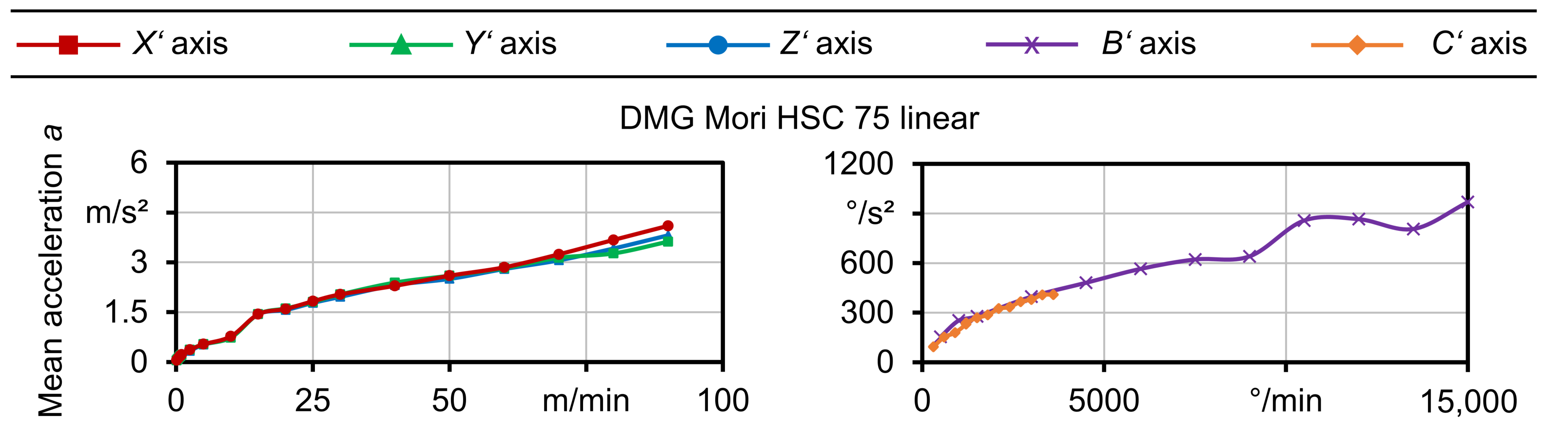
2.1.1. Machine Tool Kinematics

The kinematics of the investigated machine tool DMG Mori HSC 75 linear is shown in Figure 1. To distinguish the axis coordinates from the tool orientation B and C, the former are indicated with an apostrophe in the following. The 5-axis milling machine DMG Mori HSC 75 linear has a fork head with a swivelling milling spindle ( B axis), which performs the movements in Y and Z direction, and a rotatable workpiece table ( C axis), which traverses in X direction.
In NC programs, all process movements of cutting tools and workpieces, apart from free travel movements, are commonly described in a coordinate system relative to the workpiece, which is defined by the translatory axes X, Y and Z and spatial rotations A, B and C. Rotational and pivoting movements, which are used, e.g., to set the tool orientation, are indicated by these spatial angles. This allows NC programs to be executed on machine tools with different kinematic properties. In the control system of a machine tool, the relative coordinates are transformed into axis coordinates, which is a surjective function for 5-axis machine tools, i.e., there is no unique inverse function. A method to model the kinematic behaviour of the milling centre DMG Mori HSC 75 linear is described in the following. Due to the kinematics of the machine tool, the position of the cutting tool in relation to the workpiece influences both, the position of the B axis and the table, i.e., the C axis. Let the workpiece coordinate system be parallel to the X and Y axes of the machine tool, the position of the C axis corresponds to the angle between the transformed and non-transformed X-axis α and the position of the B’-axis corresponds to the angle ξ between the tilted tool axis z T o o l and non-tilted tool axis z , which describe the tool orientation, as shown in Figure 2. These can be determined by a transformation of the untilted tool axis z
z T o o l = R A · R B · R C · z
by the transformation matrices for rotations around the tool axes A, B and C, and R A , R B and R C , respectively. The angle ξ between the non-tilted and tilted tool axis can be calculated as
ξ = arccos z z T o o l z · z T o o l .
The angle α or C axis position, respectively, can be calculated as the angle between the tilted tool axis projected into the X Y plane by the projection matrix P and the original X axis:
α = arccos x ( P · z T o o l ) x · P · z T o o l with P :   x , y , z     x , y , 0 .
As the movement area of the B axis of the analysed machine tool is limited between + 10 B 90 and the C axis can reach every position between C = 0 and C = 360 , the B axis and C axis positions can be defined as
B   =   ξ for ξ 10 ξ else ,
C   =   α for ξ 10 α + 180 else .
To change the tool orientation, a rotation around the Tool Centre Point (TCP) is required. Due to the kinematics of the machine tool, this requires synchronous movements of the rotary and tilting axes B and C and the linear axes. Thus, the positions of the rotary and tilting axes B and C influence the position of the X axis. The positions of the Y and Z axis are influenced by the B axis position and the position of the machine table, C , respectively. The B axis position results in the influences on the axis position p B
p B   =   cos B 0 sin B 0 1 0 sin B 0 cos B · t ,
where t represents the vector from the TCP to the rotational tool axis in the unrotated coordinate system. Let w p be a vector from the centre of the machine tool table to the NC position, the table rotation C requires a shift of the linear axes positions:
p C   =   cos C sin C 0 sin C cos C 0 0 0 1 · w p .
However, the coordinates of the linear axes p A x e s can be calculated from the workpiece coordinates p W P and the shift between the workpiece coordinate system and the machine coordinate system m
p A x e s = p W P + p B + p C + m .
For the determination of the geometric properties of the machine tool, different poses in the working space were approached by defined workpiece coordinates, while the resulting axis coordinates were stored. For this, two cutting tools with different tool lengths l t were used to incorporate the tool length in the models. By solving the overdetermined system of equations obtained by inserting the values into Equation (8), t was found to be
t = 0 0 160.115   m m + l t ,
where l t is the length of the milling cutter mounted in the tool chuck and 160.115   m m is the machine specific distance between the planar support face of the clamping system and the centre of rotation of the B axis.

2.1.2. Dynamic Properties of the Axis Drives

For modelling the dynamic behaviour of the different axis drives of the machine tool, the acceleration of the linear, swivel and rotation axes X , Y , Z , B and C were individually investigated based on measurements. For this purpose, the acceleration of each axis was measured and analysed using the machine integrated position measuring system while accelerating to different feed speeds v f and decelerating to standstill, respectively. In addition, circular arcs were traversed at varying speeds in different planes to investigate the acceleration behaviour when multiple axes were moved simultaneously. A measurement frequency of f m e a s = 333.3 Hz was used, which corresponded to the maximum measurement frequency of the data recording system integrated in the control system of the machine tool. As representatively shown for the C axis of the DMG Mori HSC 75 linear and a feed velocity v f = 3600 / min (Figure 3), the acceleration showed comparable shapes and amplitudes for acceleration and deceleration phases. In all measurements, a linear increase and decrease of the acceleration was found, which indicates an acceleration with a constant jerk. The mean value of the jerk was determined from each experiment depending on the difference between start and target feed rate, as presented in Figure 4 and Table 1.
Another, simplified way to model the acceleration behaviour is the calculation with a constant acceleration value, which was determined as a function of the difference of the traverse speeds (Figure 5). To accelerate the calculation, regression models were used for modelling the acceleration of the DMG Mori HSC 75 linear, where Δ v f is given in m m / min and / min and a m , i is calculated in m m / 2 min and 2 / min , respectively:
a m , i = u · Δ v f 2 + v · Δ v f + w ,
with the parameter values of the regression models given in Table 2. The coefficient of determination was R 2 0.99 for all given regression models. In the simulations used in this research work, the model with constant acceleration was used. The acceleration model was used to calculate if the desired feed rate could be achieved. Thus, the error caused by considering the acceleration as linear could be neglected.
As presented in [27] for the linear drives of the milling centre DMG Mori HSC 75 linear, this simplification allows to calculate the achievable traverse speeds on an NC path in two steps. First, the NC path is parsed forward to calculate the axis positions and the acceleration and deceleration values of the linear drives as well as the duration for the movements of the rotary drives for each NC step. Second, the maximum achievable feed velocity for each NC step and, thus, the feed velocity along the NC path is calculated.

2.2. Geometric Physically-Based Process Simulation

Geometric physically-based cutting process simulations (GPS) [1] can be used to calculate process forces, generated workpiece surfaces [28] or tool [29] and workpiece vibrations [30]. In discrete time steps, a Constructive Solid Geometry (CSG) [31] model is applied to determine the uncut chip shape for each tooth feed by intersecting geometric models of cutting tool and workpiece. The tool model is extended by a ray-based model in order to realise a refined discrete-time calculation of the uncut chip thickness [29]. Based on the uncut chip thickness, the process forces are derived using an empirical force model based on the work in [32]. The dynamic properties of the tool are represented by a compliance model based on harmonic, uncoupled oscillators. The dynamic properties of the TCP are determined by calibrating the compliance model based on measured frequency response functions. This way, the interaction of process force and deflection and, thus, also the regenerative effect can be modelled. The pose-dependent dynamic behaviour of the system consisting of machine tool, spindle and milling tool was modelled by a linear interpolation of the oscillator parameter values (OPV) between 48 measurement poses for each time step based on the current position of the machine tool axes, as described in [16]. Based on the computed deflections between the milling tool and the workpiece, the workpiece shape is calculated by CSG modelling, while the generated surface location errors are visualised by using a multi-dexel board [33].

2.3. Approach for the Tool Orientation Dependent Optimisation of the Process Stability in 5-Axis Milling Processes

The general procedure for the pose-dependent process optimisation is shown in Figure 6.
It was carried out on the basis of a geometric model of the raw or preprocessed workpiece and an NC program with an NC path, i.e., generated by CAM, used for machining the workpiece. For the simulation of the milling process and for the collision avoidance, a geometric model of the pre-machined workpiece was utilised in the GPS in form of a triangle mesh, i.e., STL file. In order to optimise the process stability of 5-axis milling processes by changing the tool orientation, i.e., tilt and lead angle, three criteria must be verified for each position along the NC path. These were the collision avoidance, the reachability of the desired position depending on the acceleration behaviour of the machine tool and the presence of a dynamically stable state. In the GPS, a cutting force model according to Kienzle as well as a pose-dependent compliance model, described in [15], were used in order to determine positions of the axes of the spindle (B’,Y’,Z’), leading to stable and unstable processes along the NC path. The stability at a certain point of the NC path was the main criterion of the optimisation process in order to identify suitable tool orientations. Based on the Poincaré diameter (PD), which is an output variable of the GPS, the stability was evaluated. The PD describes the diameter of the path traced by a fixed point on a tool cutting edge during a complete tool rotation [34]. It was calculated for each simulation step based on the pose dependent compliance model. In case the PD exceeds 0.1 · f z , the stability criterion was exceeded and the process was declared unstable at this point. This stability criterion which was defined based on past experience well represents the sudden increase of the vibration amplitude caused by the occurrence of chatter vibrations. The application of other methods for analysing tool vibrations or determining process stability would also be possible in the presented optimisation method, for example, the methods shown in [35].
Moreover, collision data and the acceleration of the machine tool axes were simulated by using the GPS as well.
The collision monitoring was implemented as a model in the GPS similar to the work in [4]. A CSG cylinder with a diameter corresponding to the inserted tool was utilised in order to detect potential collisions of the tool shaft and the workpiece. As the workpiece and the tool intersect due to the engagement situation up to the depth of cut a p , the cylinder which determines unintentional collisions must be displaced along the tool axis in the direction of the spindle z T o o l by an offset corresponding to the tool radius. Thus, contacts between the workpiece and the spherical part of the milling tool were not considered as collisions. In order to detect and prevent collisions between the tool chuck and the workpiece, additional cylinders with the diameter corresponding to the diameter of the tool chuck and an offset corresponding to the tool length were used. Subsequently, the cylinders were tilted along the B and C axis in the GPS and the collision was checked by testing, if any workpiece point was inside the cylinder. When the cylinder was in contact with the workpiece, the maximum angle was registered and a collision cone was created from the collision-free angular positions, as shown in Figure 7.
The reachability of a potential stable and collision-free point of the NC path was evaluated on the basis of the acceleration model of the machine tool, described in Section 2.1.2. The data determined by the GPS were collected in a SQLite database. The optimiser algorithm used the database in order to identify whether the three criteria reachability, collision avoidance and process stability were fulfilled.

2.4. Optimisation Method

Predominantly, the purpose of the optimisation was to minimise the PD over the considered optimisation interval. Therefore, two approaches were considered: First, an average PD over the interval can be minimised. Second, the maximum value of the PD occurring in the interval should be minimised. An overview of the optimisation method is shown in Figure 8 and is described in detail in this section.
To collect the required data for the optimisation method, a simulation was conducted for each combination of the angle of the B and C axis which was represented by each column in the resulting diagram (Figure 9). The used range of the angle of the C axis was determined as 0 and 360 in order to allow full rotations.
Due to the axes configuration of the machine tool DMG Mori HSC 75 linear and the geometry of the workpiece, the probability of a collision in the workspace increased for B < 70 . Therefore, an interval between 70 and 0 was considered for the B rotation. Additionally, by limiting the considered interval of the B rotation, the amount of total combinations of poses was reduced as well. The stepsize within the angle intervals needed to fulfil two criteria. First, the stepsize must be high enough in order to reduce the number of necessary simulations, and second, low enough, to be reachable from the corresponding previous NC position. Thus, a stepsize of 4 was utilised for the B and C rotation, resulting in a minimal angle of B = 68 and 1620 necessary simulations. Subsequently, the collision-free tool orientations for each NC step were calculated in an additional geometric kinematic process simulation.
The NC path was split into intervals which were determined by their length as well as the direction of the motion. Therefore, a minimal, L i , m i n , and maximal interval length, L i , m a x , were used as optimisation parameters. If the direction of motion was changed in the determined interval between the min and max length, a new interval was started. In case the feed rate exceeded a certain value v f , s p l i t which indicated rapid feed movements, i.e., free travel movements, an interval was only created if the direction of motion changed as well. This was to prevent unnecessary calculation steps being performed for, e.g., travelling paths at maximum speed without tool engagement.
Using the determined intervals and the data from the simulations, a directed graph G was generated, as shown in Figure 9. For each tool orientation and interval, one node v i , B , C indexed with the interval index i and the tool orientation B and C was inserted, as well as a start and target node v s , v t , resulting in
| V | = n a n g l e s · n i n t + 2
nodes V, with the number of tool orientations n a n g l e s and intervals n i n t . Each node was filled with various data entries from the simulation output databases, containing the average and the maximum PD, the positions of the machine axes B and C and the tool orientation B and C, the interval index and an entry of the collision monitoring.
Edges were added from the start node to collision-free nodes in the first interval and from the collision-free nodes in the last interval to the target node. Other edges were only inserted for nodes in interval i to nodes in the next interval, i + 1 , by the following rule set:
  • node v i , B , C was collision-free and stable;
  • node v i + 1 , B , C was collision-free, stable and reachable; and
  • nodes in interval i + 1 , which were in between the B and C rotation of the two nodes, were collision-free, stable and reachable.
This prevented collisions and instability for each designated configuration of the B and C axis and also during the rotation process between the configurations. The reachability was checked using the acceleration models presented in Section 2.1.2. All inserted edges were weighted by
w e = P D v 0 , B , C for e = { v s , v 0 , B , C } P D v i + 1 , B , C + B = B i B i + 1 C = C i C i + 1 P D v i + 1 , B , C · w f for e = { v i , B , C , v i + 1 , B , C } , 1 i n i n t 1 1 for e = { v n i n t , B , C , v t }
using the average or maximum PD and a weight factor w f , with 68 B 0 and 0 C 356 . The inserted edges between the start node, v s , and nodes in the first interval, v 0 , B , C , were weighted by the PD of the target node of the edge. The weight of edges leading from one interval, i, to the next interval, i + 1 , were calculated by the PD of the target node of the edge, P D v i + 1 , B , C , and the sum of all PDs of nodes, whose B- and C-position was between the node in interval i and i + 1 . The weight factor, w f , was applied to penalise tool rotations of greater angles. Edges from nodes in the last interval, n i n t , to the target node, v t , were weighted by 1, because for this edge no distinction had to be made, as it did not matter which edge was used to reach the target node.
Within the constructed directed graph, a shortest path from the start node v s to the target node v t was searched with the Dijkstra path finding algorithm for directed graphs [36], resulting in a path along stable, collision-free and reachable nodes as shown in Figure 9. Afterwards, an optimised NC path could be generated using the data of the nodes along the shortest path and the related intervals.

3. Results and Discussion

In this section, the results from the GPS and the optimisation algorithm as well as an experimental validation are presented.

3.1. Simulation and Optimisation Results

An NC path for machining a free-formed workpiece was used for the validation of the optimisation algorithm. The GPS was applied to simulate the process for the selected tool orientations with the parameters presented in Table 3. The workpiece model and the investigated NC path is shown in Figure 10.
The resulting PD plot for each simulated tool orientation shows various peaks at different positions along the investigated NC path, as shown in Figure 11a). Considering the stability limit of 0.1 · f z (cf. Section 2.3), four areas with instabilities could be determined, in which several angle combinations resulted in an unstable process. Exemplary PD plots of processes with constant tool orientation are shown in Figure 11b). As indicated in the figure, no fixed tool orientation existed, which resulted in good PD values along the complete path, as the best overall PD plots still showed peaks, especially in the middle of the NC path, even if the stability limit was not exceeded.
Two exemplary optimised paths, OP1 and OP2, generated with the presented optimisation method and the parameters shown in Table 4 were also simulated with the GPS. The resulting PD plots are presented in Figure 11. In Figure 11a, the comparison between all analysed tool orientations and the optimisation results shows that the PD values from the optimised NC paths were constantly lower than the stability limit. A further peak reduction and re-movement of the optimised paths can be observed in Figure 11b), leading to one remaining peak in the NC path centre. This indicates that the presented optimisation method can effectively reduce the resulting PD to stay below the stability limit of 0.1 · f z and furthermore select suitable tool orientations for minimal tool deflection. A positive impact of the optimised tool orientation along the NC path on the resulting PD from the simulation could be determined. However, the remaining peak in the PD plot can be an indication of an unbeneficial engagement situation. By reducing the angle step value, an even better tool orientation could be found. On the other hand, this could be neglected for the presented process, as it was still stable. For other NC paths, setting smaller angle steps for the tool orientation can be necessary, which leads to a quadratic increase of the needed simulation runs. Instead of using smaller angle steps, a combination with other path optimisation methods, e.g., for adapting the cutting width and depth based on simulated process forces and tool oscillations [12], could improve the process stability.
The calculated process forces presented in frequency domain in Figure 12 showed a decrease of the forces in the low frequency range with increasing tilt angle B. In the area near the eigenfrequencies, f = 1.4–1.55 kHz, small force amplitudes around the harmonics of the tooth engagement frequency were observed, which could indicate a modulation of the uncut chip thickness and, thus, small oscillations. This effect is small, as the FFT was conducted over the whole process time. In the optimised processes, these amplitudes were lower, indicating lower oscillations between tool and workpiece. This corresponds to the lower calculated PDs.
To investigate the influence of the parameters on the optimisation process, the optimiser was run with various parameter sets, shown in Table 4. All interval length and weight factor combinations were run for each stability criterion, resulting in 182 optimised paths, which were afterwards simulated with the GPS. The computing time for one optimisation process, excluding the required simulation runs, was approximately 50 min on an AMD Ryzen 5800X processor with 32 GB of RAM. Nevertheless, the computing time for the graph generation and shortest path search varies, due to changing stability, reachability and interval lengths, leading to different amounts of intervals, nodes and edges. The method for the detection of intervals, described in Section 2.4, in some cases resulted in an equal number of intervals for different minimal and maximal interval length along the NC path (Table 4). However, even with the same number of intervals, the allocation on the NC path can be different and result in various axis angle combinations. Figure 13 shows the correlation of the weight factor, the number of intervals and the resulting mean PD value over the complete NC path for both stability criteria methods. Obviously, the mean PD value tends to decrease slightly with increasing number of intervals. A stronger effect could be identified for the decreasing weight factor, which results in lower PD values. Thus, the lowest PD values could be achieved with high interval numbers and a low weight factor. Due to the modelled pose-dependent dynamics in the simulation, the tool deflection and the PD values changed, even with fixed tool orientations. The higher interval numbers and smaller weight factors enable the optimiser to change the angles more frequently and reduce the PD values as shown in Figure 13. Therefore, a fine-stepped adjustment of the axis angles, as seen in Figure 14 for the two optimised NC paths OP1 and OP2, can have a positive impact on the process stability. On the other hand, fine-stepped changes of the tool orientation could reduce the processing and execution speed on machine tools or even cause surface location errors due to jerky movements. The weight factor, w f , was set experimentally for the investigated machining centre and needs to be set different for other machines, due to different dynamics and kinematics.
The selection of a stabilisation criterion by reducing the average or maximal PD inside one interval had minor influences on the optimisation results, as presented in Figure 13. Both methods tend to prefer a frequent adaption of the position of the B and C axis, but neither of them could be identified as the superior stability criterion for the investigated process. The previous mentioned and for stable processes preferred shorter interval length, also reduced the difference between the maximal and average PD values within each interval and therefore the influence of the stability criterion.

3.2. Validation Experiments

Validation experiments were conducted on the 5-axis machining centre DMG Mori HSC 75 linear for the two processes OP1 and OP2 optimised by average and maximal PD criterion, respectively, as well as reference processes with different constant tool orientations (Figure 15). During the milling experiments, the acoustic emissions and process forces were measured using a Tascam DR-40 audio recorder and a dynamometer Kistler type 9255B, on which the workpiece was mounted using a tailored chuck. The processes were conducted with a constant spindle speed n = 2196 / min and a feed per tooth f z = 0.085   m m . During long rotational movements of the B and C axes, the feed velocity was automatically reduced by the control system of the machine tool to comply with the specified path tolerance and to achieve a better surface quality. As a result, the duration of the optimised processes was slightly extended.
The process forces (Figure 16) measured in three Cartesian directions were filtered using a low-pass filter with a cut-off frequency of f c = 2 k Hz in a charge amplifier Kistler 5070A and recorded with a measurement frequency of f m e a s = 25.6 k Hz . The process forces of the whole process were summed up to calculate the total force
F g e s = F x 2 + F y 2 + F z 2
and transformed to the frequency domain by Fast Fourier Transformation (FFT) with a rectangular window function calculating RMS values. Due to the measurement characteristics of the dynamometer especially at higher frequencies, the absolute force values cannot be guaranteed to be accurate. For this reason and others, e.g., due to the parameterisation of the underlying process force model and process damping effects not represented in the simulation, deviations between measured and simulated process forces could have occurred. As all measurements were conducted in the same setup, they can still be compared with each other.
For the processes with low constant tilt angle B = 4 , the highest forces were measured as a result of the comparatively low effective cutting speed. For the optimised processes, the process forces at frequencies f 160 Hz were comparable to the forces measured at B = 56 . For higher frequencies, they were lower compared to the processes with constant tool orientation. Overall, the measured process forces showed the same behaviour as the simulated forces (cf. Figure 12). Only the DC component deviated from the simulated forces by a factor of about three. The presence of slightly increased force amplitudes at the harmonics of the tooth engagement frequency f z near the eigenfrequencies of the milling tool in the area f = 1.4–1.55 kHz which occurred in the process with constant tool orientation B = 56 indicated slight oscillations. In the optimised processes OP1 and OP2, the measured forces in this frequency range were lower. This effect was very small because the FFT was carried out over the entire process duration, so that a short-term occurrence of oscillations only caused a small increase in the corresponding amplitudes. However, the low level of this effect does not indicate whether it is relevant in practice.
The acoustic emissions (Figure 17) measured with rotating spindle showed increased signal amplitudes at the frequency f = 1355 Hz which were generated without any tool engagement. Thus, this frequency cannot be used to determine the process stability or chatter, respectively. The processes with constant tool orientation showed increased signal amplitudes at the harmonics of the tooth engagement frequency in the area near the eigenfrequencies of the tool–machine system around f 1400 Hz and f 1530 Hz over the whole processes. Especially for the processes with low tilt angle B, the amplitudes were significantly higher than those at the tooth engagement frequency, indicating chatter vibrations with low amplitudes. In the concave areas of the workpiece surface, e.g., at the beginning of the NC path, these increased amplitudes were most distinctive due to the higher wrap angle. In contrast, for the optimised processes, increased amplitudes of the acoustic emissions were only observed in some areas of the workpiece. Especially in the concave areas of the workpiece, in which the simulation predicted the highest PDs, i.e., (cf. Figure 13), the acoustic emissions were lower compared to the processes with constant tool orientation. The measurements therefore indicate an improvement of the process with regard to the occurrence of vibrations. This is opposed to an increase of the process time, which could be countered with an increase of the depth of cut or the feed rate. Comparing both optimisation strategies, the process OP2, which was optimised based on the maximal PD, showed lower process forces and acoustic emissions. This optimisation criterion could, therefore, be evaluated as more suitable for the presented application.

4. Conclusions

In this paper, a method for optimising process stability by taking advantage of the axis position-dependent dynamic behaviour of machine tools and the flexible usability of spherical milling tools in a simultaneous 5-axis milling process was presented. The main criterion of the process stability for discrete positions along the NC path, as well as the two constraints of the reachability of the desired axis position and the collision-free swivelling into the corresponding position, were taken into account. An experimentable digital twin of an exemplary machining centre consisting of an axis position-dependent compliance model based on empirical data and kinematic and dynamic models was integrated in a geometric physically-based process simulation system. Simulation-based process optimisation was carried out by the presented optimisation method. To find tool orientations along an NC path suitable to achieve a stable milling process, processes were simulated with different combinations of machine axis angles. The PD was used as a stability criterion. By separating the NC path into intervals defined by their length and changes of the feed direction, nodes for a directed graph could be generated. In this, a path could be searched which led to a stable process by evaluating the maximum or average PD. To ensure the reachability of the identified stable positions of the rotational axes, an empirical acceleration model in combination with a kinematic model was used for the simulation process. By using a penalty function for both axis rotations and the PD, axis rotations could be constrained while a stable process could be achieved.
A simulation-based study of the interval length and weighting parameters resulted in lower PDs with shorter interval length and lower penalisation of axis rotations. On the other hand, higher calculation times were needed due to a refinement of the angle steps required for optimisation with shorter interval length. The optimisation of an exemplary process resulted in a significant reduction of the PD along the entire NC path.
Validation experiments conducted for the optimised processes showed a reduction of the process forces in the range of the eigenfrequencies of the system in most areas of the NC path, corresponding to the simulation results. Measurements of the acoustic emissions also showed lower amplitudes, i.e., oscillations, in these frequencies. Thus, it could be shown that the presented optimisation algorithm can lead to an improvement of 5-axis milling processes. In the future, further improvements could be achieved by incorporating additional process parameters, such as the feed rate, into the optimisation. On the other hand, this would also increase the computational effort and memory requirements.
Although the presented simulation-based optimisation led to good results, its applicability is limited by the complex empirically-based model parameterisation. The calibration of the used pose-dependent compliance model and process force model for spherical milling tools implies a high experimental effort. As the process force calculation and simulation of the tool deflections using a compliance model directly influence each other, a new method for the model calibration should be developed. Combined measurements of process forces and deflections of the tool in milling processes could be performed to facilitate the model parameterisation and further improve the simulation results.

Author Contributions

Conceptualisation, P.W., I.W., A.W. and T.M.; methodology, P.W. and T.M.; software, T.M.; validation, A.W. and T.M.; formal analysis, T.M.; investigation, P.W., I.W., A.W. and T.M.; resources, D.B. and P.W.; data curation, T.M.; writing—original draft preparation, I.W., A.W. and T.M.; writing—review and editing, P.W., D.B., I.W., A.W. and T.M.; visualisation, I.W., A.W. and T.M.; supervision, D.B. and P.W.; project administration, D.B. and P.W.; funding acquisition, D.B. and P.W. All authors have read and agreed to the published version of the manuscript.

Funding

Gefördert durch die Deutsche Forschungsgemeinschaft (DFG)-403392440. Funded by the Deutsche Forschungsgemeinschaft (DFG, German Research Foundation)-403392440.

Data Availability Statement

No new data were created or analysed in this study. Data sharing is not applicable to this article.

Acknowledgments

We acknowledge financial support by Deutsche Forschungsgemeinschaft and Technische Universität Dortmund/TU Dortmund University within the funding programme Open Access Publishing. Furthermore, the authors gratefully acknowledge the computing time provided on the Linux HPC cluster at TU Dortmund University (LiDO3), partially funded in the course of the Large-Scale Equipment Initiative by the German Research Foundation (DFG) as project 271512359.

Conflicts of Interest

The authors declare no conflict of interest. The funders had no role in the design of the study or in the writing of the manuscript.

Abbreviations

The following abbreviations are used in this manuscript:
CADComputer-Aided Design
CAMComputer-Aided Manufacturing/Machining
CSGConstructive Solid Geometry
FFTFast Fourier Transformation
FRFFrequency Response Function
GPSGeometric physically-based Process Simulation
MDPIMultidisciplinary Digital Publishing Institute
PDPoincaré Diameter
TCPTool Centre Point

References

  1. Wiederkehr, P.; Siebrecht, T. Virtual Machining: Capabilities and Challenges of Process Simulations in the Aerospace Industry. Procedia Manuf. 2016, 6, 80–87. [Google Scholar] [CrossRef] [Green Version]
  2. Weinert, K.; Enselmann, A.; Friedhoff, J. Milling Simulation for Process Optimization in the Field of Die and Mould Manufacturing. CIRP Ann. 1997, 46, 325–328. [Google Scholar] [CrossRef]
  3. Ozturk, E.; Budak, E. Modeling of 5-axis milling processes. Mach. Sci. Technol. 2007, 11, 287–311. [Google Scholar] [CrossRef]
  4. Kersting, P.; Zabel, A. Optimizing NC-tool paths for simultaneous five-axis milling based on multi-population multi-objective evolutionary algorithms. Adv. Eng. Softw. 2009, 40, 452–463. [Google Scholar] [CrossRef]
  5. Altintaş, Y.; Budak, E. Analytical Prediction of Stability Lobes in Milling. CIRP Ann.-Manuf. Technol. 1995, 44, 357–362. [Google Scholar] [CrossRef]
  6. Altintaş, Y.; Kersting, P.; Biermann, D.; Budak, E.; Denkena, B.; Lazoglu, I. Virtual process systems for part machining operations. CIRP Ann. 2014, 63, 585–605. [Google Scholar] [CrossRef]
  7. Shamoto, E.; Akazawa, K. Analytical prediction of chatter stability in ball end milling with tool inclination. CIRP Ann. 2009, 58, 351–354. [Google Scholar] [CrossRef]
  8. Lazoglu, I.; Liang, S.Y. Analytical modeling of force system in ball-end milling. Mach. Sci. Technol. 1997, 1, 219–234. [Google Scholar] [CrossRef]
  9. Budak, E.; Ozturk, E. Chatter Stability of 5-Axis-Milling Using Multi-Frequency Solution. In Proceedings of the 3rd International Conference on High Performance Cutting, Dublin, Ireland, 12–13 June 2008; pp. 429–444. [Google Scholar]
  10. Budak, E.; Ozturk, E.; Tunc, L.T. Modeling and simulation of 5-axis milling processes. CIRP Ann.-Manuf. Technol. 2009, 58, 347–350. [Google Scholar] [CrossRef] [Green Version]
  11. Sun, C.; Altintaş, Y. Chatter free tool orientations in 5-axis ball-end milling. Int. J. Mach. Tools Manuf. 2016, 106, 89–97. [Google Scholar] [CrossRef]
  12. Tunc, L.T. Smart tool path generation for 5-axis ball-end milling of sculptured surfaces using process models. Robot.-Comput.-Integr. Manuf. 2019, 56, 212–221. [Google Scholar] [CrossRef]
  13. Baumann, J.; Siebrecht, T.; Wiederkehr, P. Modelling the Dynamic Behavior of a Machine Tool Considering the Tool-position-dependent Change of Modal Parameters in a Geometric-kinematic Simulation System. Procedia CIRP 2017, 62, 351–356. [Google Scholar] [CrossRef]
  14. Brecher, C.; Altstädter, H.; Daniels, M. Axis Position Dependent Dynamics of Multi-axis Milling Machines. Procedia CIRP 2015, 31, 508–514. [Google Scholar] [CrossRef] [Green Version]
  15. Wirtz, A.; Wilck, I.; Schmidt, N.; Biermann, D.; Wiederkehr, P. Experimental analysis of tilt-angle dependent dynamic properties of a 5-axis milling center. Manuf. Lett. 2021, 29, 47–51. [Google Scholar] [CrossRef]
  16. Wilck, I.; Wirtz, A.; Biermann, D.; Wiederkehr, P. Application of interpolation methods for the determination of position-dependent frequency response functions for the simulation of five-axis milling processes. Prod. Eng. 2021, 15, 10. [Google Scholar] [CrossRef]
  17. Finkeldey, F.; Wirtz, A.; Merhofe, T.; Wiederkehr, P. Learning-Based Prediction of Pose-Dependent Dynamics. J. Manuf. Mater. Process. 2020, 4, 85. [Google Scholar] [CrossRef]
  18. Zhao, Z.Y.; Wang, C.Y.; Wu, S.X.; Zhou, H.M. Tool path optimization of pocket corner. Trans. Nanjing Univ. Aeronaut. Astronaut. 2007, 24, 164–169. [Google Scholar]
  19. Kolar, P.; Sulitka, M.; Matyska, V.; Fojtu, P. Optimization of five-axis finish milling using a virtual machine tool. MM Sci. J. 2019, 2019, 3534–3543. [Google Scholar] [CrossRef] [Green Version]
  20. Tandon, V.; El-Mounayri, H.; Kishawy, H. NC end milling optimization using evolutionary computation. Int. J. Mach. Tools Manuf. 2002, 42, 595–605. [Google Scholar] [CrossRef]
  21. Brecher, C.; Fey, M.; Daniels, M. Modeling of Position-, Tool- and Workpiece-Dependent Milling Machine Dynamics. High Speed Mach. 2016, 2, 15–25. [Google Scholar] [CrossRef]
  22. Anotaipaiboon, W.; Makhanov, S.S. Tool path generation for five-axis NC machining using adaptive space-filling curves. Int. J. Prod. Res. 2005, 43, 1643–1665. [Google Scholar] [CrossRef]
  23. Jha, N.K.; Hornik, K. Integrated computer-aided optimal design and finite element analysis of a plain milling cutter. Appl. Math. Model. 1995, 19, 343–353. [Google Scholar] [CrossRef] [Green Version]
  24. Huang, T.; Zhang, X.M.; Ding, H. Tool Orientation Optimization for Reduction of Vibration and Deformation in Ball-end Milling of Thin-walled Impeller Blades. Procedia CIRP 2017, 58, 210–215. [Google Scholar] [CrossRef]
  25. Kayhan, M.; Budak, E. An experimental investigation of chatter effects on tool life. Proc. Inst. Mech. Eng. Part B J. Eng. Manuf. 2009, 223, 1455–1463. [Google Scholar] [CrossRef] [Green Version]
  26. Munoa, J.; Beudaert, X.; Dombovari, Z.; Altintas, Y.; Budak, E.; Brecher, C.; Stepan, G. Chatter suppression techniques in metal cutting. CIRP Ann.-Manuf. Technol. 2016, 65, 785–808. [Google Scholar] [CrossRef]
  27. Biermann, D.; Wiederkehr, P.; Hensel, M.; Freiburg, D.; Finkeldey, F. Simulation of surface structuring considering the acceleration behaviour by means of spindle control. Int. J. Mechatron. Manuf. Syst. 2018, 11, 67–86. [Google Scholar] [CrossRef]
  28. Siebrecht, T.; Kersting, P.; Biermann, D.; Odendahl, S.; Bergmann, J. Modeling of Surface Location Errors in a Multi-scale Milling Simulation System Using a Tool Model Based on Triangle Meshes. Procedia CIRP 2015, 37, 188–192. [Google Scholar] [CrossRef]
  29. Surmann, T.; Enk, D. Simulation of milling tool vibration trajectories along changing engagement conditions. Int. J. Mach. Tools Manuf. 2007, 47, 1442–1448. [Google Scholar] [CrossRef]
  30. Biermann, D.; Kersting, P.; Surmann, T. A general approach to simulating workpiece vibrations during five-axis milling of turbine blades. CIRP Ann. 2010, 59, 125–128. [Google Scholar] [CrossRef]
  31. Foley, J.D.; van Dam, A.; Feiner, S.K.; Hughes, J.F. Computer Graphics: Principles and Practice, Reprinted with Corrections, July 1997 ed., 2nd ed.; Addison-Wesley Publishing Company, Inc.: Boston, MA, USA, 1997. [Google Scholar]
  32. Kienzle, O. Die Bestimmung von Kräften und Leistungen an spanenden Werkzeugen und Werkzeugmaschinen. VDI-Z 1952, 94, 299–305. [Google Scholar]
  33. Müller, H.; Surmann, T.; Stautner, M.; Albersmann, F.; Weinert, K. Online Sculpting and Visualization of Multi-Dexel Volumes. In Proceedings of the 8th ACM Symposium on Solid Modeling and Applications, Seattle, WA, USA, 16–20 June 2003; pp. 258–261. [Google Scholar]
  34. Davies, M.A.; Dutterer, B.; Pratt, J.R.; Schaut, A.; Bryan, J. On the dynamics of high-speed milling with long, slender endmills. CIRP Ann. 1998, 47, 55–60. [Google Scholar] [CrossRef]
  35. Niu, J.; Ding, Y.; Geng, Z.; Zhu, L.; Ding, H. Patterns of Regenerative Milling Chatter Under Joint Influences of Cutting Parameters, Tool Geometries, and Runout. J. Manuf. Sci. Eng. 2018, 140, 121004. [Google Scholar] [CrossRef]
  36. Dijkstra, E.W. A note on two problems in connexion with graphs. Numer. Math. 1959, 1, 269–271. [Google Scholar] [CrossRef] [Green Version]
Figure 1. Machine tool kinematics of the 5-axis milling machine DMG Mori HSC 75 linear.
Jmmp 05 00099 g001
Figure 2. Description of the tool orientation in (a) 3D view and (b) top view.
Jmmp 05 00099 g002
Figure 3. (a) Positioning from C = 0 to C = 45 with Δ v f = 3600 / min and (b) linear increase of the acceleration due to a constant jerk.
Jmmp 05 00099 g003
Figure 4. Mean jerk values measured while accelerating from standstill in dependence of the target feed rate for the machining centre DMG Mori HSC 75 linear.
Jmmp 05 00099 g004
Figure 5. Modelling of the acceleration by the measured mean acceleration a as a function of the feed rate difference between the current and former NC step for the machine tool DMG Mori HSC 75 linear.
Jmmp 05 00099 g005
Figure 6. Approach for process stability optimisation using tilt angle-dependent compliance models.
Jmmp 05 00099 g006
Figure 7. Principle of the collision avoidance between workpiece, toolholder and tool, cf. [4], showing (a) the calculated collison cone, with collision-free rotations. In (b) the tilted cylinders within the simulation are shown, marking the maximal collision-free angles.
Jmmp 05 00099 g007
Figure 8. Principle of the optimisation method.
Jmmp 05 00099 g008
Figure 9. Resulting tool orientation from the optimisation for each point of the NC path.
Jmmp 05 00099 g009
Figure 10. Analysed NC path for optimisation: (a) in X- and Z-coordinates and (b) in the GPS, showing the prepared workpiece model.
Jmmp 05 00099 g010
Figure 11. (a) PD plots for all analysed tool orientations and two optimised paths. (b) Mean PD plots of exemplary processes with constant tool orientations and the two processes with optimised tool orientations.
Jmmp 05 00099 g011
Figure 12. Root Mean Square (RMS) values of the simulated process forces over the whole process for (a,c) fixed B and C orientation and (b,d) two optimised paths.
Jmmp 05 00099 g012
Figure 13. Resulting simulated mean Poincaré diameter of optimised NC paths with various parameters using (a) the average PD and (b) the max PD as stability criteria.
Jmmp 05 00099 g013
Figure 14. Angle of (a) B and (b) C axis adjustment along the optimised NC paths OP1 and OP2.
Jmmp 05 00099 g014
Figure 15. Workpiece used in the validation experiments.
Jmmp 05 00099 g015
Figure 16. RMS values of the process forces measured in the validation experiments for (a,c) fixed B and C orientation and (b,d) two optimised paths.
Jmmp 05 00099 g016
Figure 17. Acoustic emissions measured in the validation experiments.
Jmmp 05 00099 g017
Table 1. Maximum jerk values measured for the axis drives.
AxisJerk
B 10.65 / s 3
C 12.98 / s 3
X 14.72   m / s 3 for v f , X 10   m / min
34.70   m / s 3 for v f , X 15   m / min
Y 14.77   m / s 3 for v f , Y 10   m / min
34.72   m / s 3 for v f , Y 15   m / min
Z 14.58   m / s 3 for v f , Z 10   m / min
34.56   m / s 3 for v f , Z 15   m / min
Table 2. Parameter values of the acceleration model.
Axisu in /mmv in /minw in mm 2 /minfor v f in mm 2 /min
0.0 715.81 106,4000 Δ v f < 1000
X’ 0.017 389.7 52,6561000 Δ v f 10,000
0.0004322 146.01 648,87410,000 < Δ v f
0.0 705.5 147,1610 Δ v f < 1000
Y’ 0.013 358.5 407,9031000 Δ v f 10,000
0.0002739 106.3 3,670,05210,000 < Δ v f
0.0 701.08 139,1960 Δ v f < 1000
Z’ 0.013 357.2 471,4821000 Δ v f 10,000
0.0002739 194.3 3,901,53610,000 < Δ v f
Table 3. Parameter values of the milling process.
ParameterValue
StrategyDown milling
Tool diameter d = 10   m m
Depth of cut a p = 0.3   m m
Width of cut a e = 0.0–0.2 mm
Spindle speed n = 2196   min 1
Feed per tooth f z = 0.085   m m
Table 4. Optimisation parameters.
ParameterValues
Stability criterionavg., max.
Stability limit 0.0085   m m
Weight factor w f 0.01 , 0.05 , 0.1 , 0.5 , 1, 2, 5
Min. interval length L i , m i n in m m 5522211
Max. interval length L i , m a x in m m 151085654
No. of intervals n i n t 18193738386263
Min. interval length L i , m i n in m m 10.50.50.50.50.2
Max. interval length L i , m a x in m m 332.521.51.5
No. of intervals n i n t 657376808585
Optimised PathStability criterionStability limit w f L i , m i n L i , m a x
“OP1”avg. 0.0085   m m 0.1 2   m m 5   m m
“OP2”max. 0.0085   m m 0.01 0.5   m m 2   m m
Publisher’s Note: MDPI stays neutral with regard to jurisdictional claims in published maps and institutional affiliations.

