Article

Fault Detection and Fault-Tolerant Cooperative Control of Multi-UAVs under Actuator Faults, Sensor Faults, and Wind Disturbances

1
College of Automation Engineering, Nanjing University of Aeronautics and Astronautics, Nanjing 211106, China
2
Mechanical, Industrial and Aerospace Engineering, Concordia University, Montreal, QC H3G 1M8, Canada
*
Author to whom correspondence should be addressed.
Drones 2023, 7(8), 503; https://doi.org/10.3390/drones7080503
Submission received: 3 July 2023 / Revised: 24 July 2023 / Accepted: 27 July 2023 / Published: 1 August 2023

Abstract

:
Fault detection (FD) and fault-tolerant cooperative control (FTCC) strategies are proposed in this paper for multiple fixed-wing unmanned aerial vehicles (UAVs) under actuator faults, sensor faults, and wind disturbances. Firstly, the faulty model is introduced while the effectiveness loss, deviation of thrust throttle setting, and pitot sensor faults are considered. Secondly, the faulty UAV model with wind disturbances is linearized and the system is then converted into two subsystems by using state and output transformations. Further, cooperative unknown input observers (UIOs) are developed to estimate the faults, disturbances, and states. By combining with the observers’ estimations, adaptive thresholds are designed to detect actuator and sensor faults in the system. Then, considering state constraints, a backstepping-based FTCC scheme is proposed for multiple UAVs (multi-UAVs) suffering from actuator faults, sensor faults, and wind disturbances. It is shown by Lyapunov analysis that the tracking errors are fixed-time convergent. Finally, the effectiveness of the FD and FTCC scheme is verified by numerical simulation.

1. Introduction

Due to low cost and flexible deployment characteristics, unmanned aerial vehicles (UAVs) have been increasingly, and more widely, used in numerous fields, such as forest fire monitoring [1,2], search and rescue [3], and power grid inspection [4]. Among these uses, fixed-wing UAVs have been widely used in wide-area coverage search [5], long-distance logistics transportation [6], and communication relays [7], due to their strong carrying capacity, fast flight speed, and long endurance.
With the development of UAV autonomous technology, cooperative control of multiple UAVs (multi-UAVs) has become an important research direction [8,9,10,11,12]. Through cooperative operations, multi-UAVs demonstrate high task execution efficiency, superior coordination, intelligence, and autonomy. To ensure the cooperative control performance of multi-UAV systems during mission execution, operational safety has become a hot research issue in the field of flight control. When multi-UAVs cooperate in performing tasks, such as environmental monitoring, fire monitoring, and collaborative search, there is a risk of losing control of the faulty UAVs if one or more UAVs encounter physical faults. In severe cases, the faulty UAVs may collide with surrounding UAVs, resulting in the entire flight formation losing control. Therefore, studying the problem of fault detection (FD), fault estimation, and fault-tolerant cooperative control (FTCC) is of great theoretical significance and practical necessity for the safe flight of monitoring missions and the safe control of multi-UAV systems.
It is worth noting that, with increases in operating time, environmental complexity, and severity, actuators and sensors may experience wear and aging. Furthermore, in the cooperative formation flight of multi-UAVs, the number of system components in the entire system significantly increases. The multi-UAVs system involves communication network connections, which provide the faulty UAVs with the opportunity to send perturbed state information to all nearby UAVs, greatly increasing the probability of collision and failure of the mission undertaken. Compared with the FD and fault-tolerant control (FTC) for single UAVs, the FD and FTCC for multi-UAVs are increasingly complicated. In addition, the external disturbances encountered by UAVs and the system nonlinearity also pose great challenges and difficulties in researching multi-UAVs. How to detect various faults in a multi-UAV system affected by disturbances, and to deal with the faults effectively, have become significant research topics to ensure the safe and cooperative formation flight of multi-UAVs.
In order to discover faults in the system in a timely and accurate manner, many scholars have carried out extensive research on this topic [13,14,15,16]. In [17], two sensor fault estimation schemes were proposed for a class of nonlinear systems with uncertainties, which were then applied to satellite control systems. The incipient fault diagnosis of a class of Lipschitz nonlinear systems was studied in [18]. By constructing total measurable fault information residual (ToMFIR), the incipient faults of multiple sensors can be detected. The linear descriptor reduced-order observer and descriptor sliding-mode observer were proposed to solve the state and fault estimation problems of linear systems with disturbances, sensor and actuator faults in [19]. Nevertheless, the FD results on multi-UAV systems with actuators and sensor faults and disturbances are very rare.
In practical situations, the consideration of a state constraint is very important for UAVs, since this consideration can simultaneously prevent the occurrence of accidents, ensure the safety of UAVs, improve system stability, enhance performance and efficiency, and reduce energy consumption during flight. In recent years, some methods have been proposed in regard to constraint control problems, including the invariant-set method [20,21], model predictive control (MPC) [22,23], and barrier Lyapunov function (BLF) [24,25], etc. A distributed FTC method and state transformations with the scaling function were proposed for fixed-wing UAVs subject to actuator faults and full state constraints, maintaining speed and attitude within the corresponding constraint ranges [26]. In [27], an adaptive FTC scheme, based on reinforcement learning and barrier Lyapunov control technology, was designed to solve the attitude tracking problem of flying-wing UAVs under actuator fault, actuator saturation, and attitude angle constraints. A novel integral barrier Lyapunov function (IBLF) was proposed for the FTC of fixed-wing UAVs with asymmetric time-varying full state constraints [28]. Nevertheless, the state constraint problem of multiple fixed-wing UAVs is rarely considered, which needs further investigations.
To better improve the cooperative operation performance of the entire multi-UAV system, numerous researchers have achieved a quantity of exploratory FTCC results. At present, FTCC schemes are mainly developed based on the leader–follower formation [29,30,31] and distributed communication architectures [32,33,34]. In [35], a dynamic surface fixed-time FTC scheme, based on a neoteric disturbance observer, was proposed for fixed-wing UAVs against actuator faults and external disturbances. A fault detection observer was proposed by using the H method for sensor faults in a multi-UAV system. Then, a distributed fault-tolerant formation controller was designed in [36]. In [37], by using intelligent learning architecture and fractional-order calculus, an FTCC strategy was proposed for multiple fixed-wing UAVs with actuator and sensor faults. In addition, there is a high demand to design fixed-time FTCC schemes to ensure rapid fault tolerance.
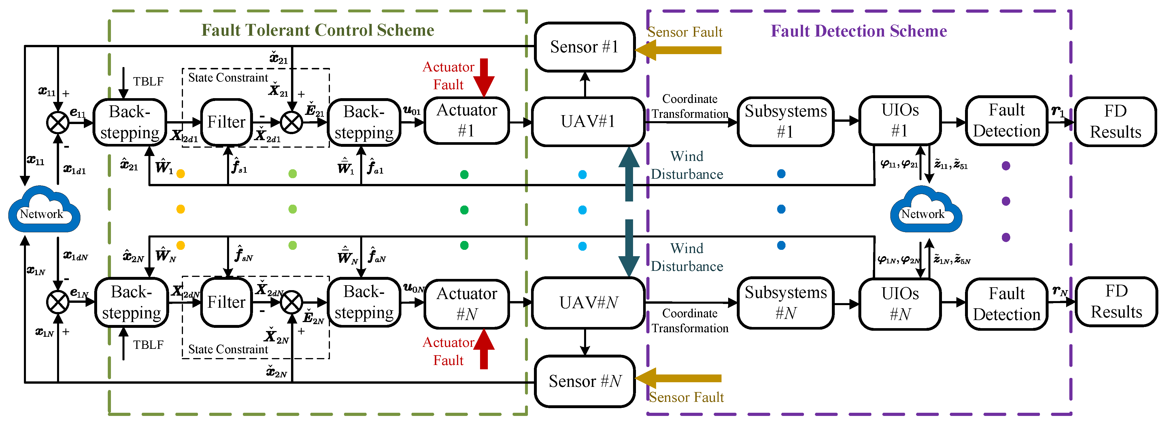
Based on the above discussions, in this paper, the FD and FTCC strategy are proposed to solve the cooperative control problem of multiple fixed-wing UAVs with actuator faults, sensor faults, and wind disturbances. The contributions of this paper are mainly as follows.
1.
Compared with the previous results on FD and fault estimation methods in [17,18,19], a newly constructed cooperative unknown input observer (UIO) is developed to estimate states, faults, and disturbances. Combined with the observers’ estimations, adaptive thresholds are designed to detect actuator and sensor faults in the system.
2.
Tangential barrier Lyapunov function (TBLF) is combined with the state transformation with scaling function to constrain the states.
3.
Differing from existing FTC strategies for fixed-wing UAVs [35,36,37], a backstepping-based fixed-time FTCC scheme is proposed for multi-UAVs suffering from actuator faults, sensor faults, and wind disturbances.
The rest of this paper is organized as follows. Section 2 introduces the fixed-wing UAV models with wind disturbances, actuator fault, sensor fault, and the preliminaries for controller design. FD and fault estimation schemes are proposed in Section 3. An FTCC scheme is designed in Section 4. Section 5 illustrates the simulation results. Conclusions are presented in Section 6.

2. Preliminaries and Problem Statement

2.1. UAV Dynamics

In this paper, a group of fixed-wing follower UAVs and a virtual leader are considered. The dynamic model of the follower UAV#i with wind disturbances is given as follows [38]:
x ˙ i = V i cos γ i cos χ i + W x y ˙ i = V i cos γ i sin χ i + W y z ˙ i = V i sin γ i + W z
where  p i = [ x i , y i , z i ] T  is the position of the UAV # i  in the inertial frame for  i 1 , 2 , , N V i χ i , and  γ i  denote the velocity, heading angle, and flight path angle, respectively.  W x W y , and  W z  are the components of the wind speed vector along the x, y and z axes of the inertial coordinate system.
The force equations are expressed as:
V ˙ i = D i + T i / m g sin γ i W ˙ x cos γ i cos χ i W ˙ y cos γ i sin χ i W ˙ z sin γ i χ ˙ i = L i sin ϕ i / m V i cos γ i + W ˙ x sin χ i W ˙ y cos χ i / V i cos γ i γ ˙ i = L i cos ϕ i / m V i m g cos γ i / V i + W ˙ x sin γ i cos χ i + W ˙ y sin γ i sin χ i W ˙ z cos γ i / V i
where m and g are the mass and gravitational constant, respectively.  T i D i , and  L i  represent the thrust, drag, and lift forces, respectively.  ϕ i  denotes the bank angle.
The forces  T i  and  D i  are described as:
T i = T m a x δ t i D i = q ¯ i s i C i D 0
where  T m a x  and  δ t i  denote the maximal engine thrust force and instantaneous thrust throttle setting, respectively. The value  q ¯ i = 1 / 2 ρ V i 2  denotes the the dynamic pressure and  ρ  is the air density,  s i  denotes the wing area.  C i D 0  is the aerodynamic coefficient.
Define  x 1 i = x i , y i , h i T , x 2 i = V i , χ i , γ i T u i = δ t i , ϕ i , L i T , one has:
x ˙ 1 i = F 1 i + G 1 i x 2 i + W i x ˙ 2 i = F 2 i + G 2 i u i + W ¯ i
where  F 1 i G 1 i F 2 i G 2 i W i W ¯ i  are given as
F 1 i = V i cos γ i cos χ i V i V i cos γ i sin χ i χ i V i sin γ i γ i G 1 i = 1 0 0 0 1 0 0 0 1 ,
F 2 i = D i / m g sin γ i L i sin ϕ i / m V i cos γ i ϕ i L i cos ϕ i / m V i g cos γ i / V i L i G 2 i = T max / m 0 0 0 1 0 0 0 1 ,
W i = W x W y W z W ¯ i = W ˙ x cos γ i cos χ i W ˙ y cos γ i sin χ i W ˙ z sin γ i W ˙ x sin χ i W ˙ y cos χ i / V i cos γ i W ˙ x sin γ i cos χ i + W ˙ y sin γ i sin χ i W ˙ z cos γ i / V i .

2.2. Faulty UAV Model

Actuator and sensor faults may give rise to the degradation of flight performance and affect the safety of the formation team. The thrust output of the engine may differ from the expected value due to wear or fault of the engine. Pitot may be faulty due to environmental erosion or influence. For the above reasons, we considered the effectiveness loss, deviation of thrust throttle setting, and pitot faults in this paper, given as  δ t i = ρ t i δ t 0 i + δ t b i  and  V s i = ϱ v i V i + V b i . Thus, the following fault models are obtained [37]:
u i = ρ i u 0 i + u b i = u 0 i + f a i
where  u i  and  u 0 i = [ u 01 i , u 02 i , u 03 i ] T  denote the applied and commanded control input signals, respectively.  ρ i = diag ρ t i , 1 , 1 , ρ t i ( 0 , 1 ]  denotes the control effectiveness.  u b i = [ δ t b i , 0 , 0 ] T  denotes the deviation value.  f a i = ρ i I u 0 i + u b i = f a 1 i , f a 2 i , f a 3 i T .
x ˇ 2 i = ϱ i x 2 i + x b i = x 2 i + f s i
where  x ˇ 2 i  and  x 2 i  denote the measured and real state signals, respectively.  ϱ i = diag ϱ v i , 1 , 1 ϱ v i ( 0 , 1 ]  denotes the measurement effectiveness.  x b i = [ V b i , 0 , 0 ] T  denotes the deviation value.  f s i = ϱ i I x 2 i + x b i = f s 1 i , f s 2 i , f s 3 i T .
By substituting (5) and (6) into (4), the faulty UAV model is presented as:
x ˙ 1 i = F 1 i + G 1 i x ˇ 2 i ϱ i I x 2 i x b i + W i x ˇ ˙ 2 i = F 2 i + G 2 i ρ i u 0 i + u b i + ϱ i I F 2 i + G 2 i ρ i u 0 i + u b i + ϱ i x 2 i + x ˙ b i + W ¯ i

2.3. Communication Network

Leader and N follower UAVs were considered in the multi-UAV system. The communication network among the follower UAVs is presented by an undirected topology  G υ , ε , where  υ = 1 , 2 , , N  is a set of follower UAVs and  ε υ × υ  is an edge set. If  i , j ε , the jth UAV is a neighbor of the ith UAV.  Ω i = j υ i , j ε  is the neighborhood set of the ith UAV. The adjacency matrix  A = a i j R N × N  is given by  a i j = 1  if  i , j ε  and  a i j = 0  otherwise. The Laplacian matrix  L D A , where  D = diag Γ i R N × N  with  Γ i = j Ω i a i j . Furthermore, the leader adjacency matrix  C = diag c 1 , c 2 , , c N  is given by  c i = 1  if the ith UAV can obtain the information of the leader and  c i = 0  otherwise.

2.4. Control Objective

FD and FTCC scheme for multiple fixed-wing UAVs against actuator faults, sensor faults and wind disturbances are proposed in this paper and the objectives are listed as follows: (a) The actuator faults and sensor faults to be detected by the fault detection scheme; (b) The faults and wind disturbances to be estimated by the developed cooperative UIOs; (c) The desired cooperative formation flight can be kept by the designed FTCC scheme.
The following assumptions and lemmas may be used for the FD and FTCC designs.
Assumption 1. 
The communication network of multi-UAVs system is undirected and connected.
Lemma 1 
([39]). Consider the system  x ˙ = f x t , x 0 = x 0 . If there exists a Lyapunov function  V x  and constants  α > 0 β > 0 p > 1 0 < q < 1 , and  0 < ϖ <  such that:
V ˙ x α V p x β V q x + ϖ
Then, the system is practically fixed-time stable. The settling time T is presented as  T T max = 1 α ϕ p 1 + 1 β ϕ 1 q  with  0 < ϕ < 1 . The convergence neighborhood is given by:
x V x min ϖ 1 ϕ α 1 p , ϖ 1 ϕ β 1 q .

3. Fault Detection and Estimation Scheme Design

By using the feedback linearization, the fixed-wing UAV model (1)–(2) in the presence of actuator and sensor faults can be rewritten as:
X ˙ i t = AX i t + Bu 0 i t + M η i t , X i , u 0 i + Dd i t , X i + E f a 1 i t y i t = CX i t + F f s 1 i t
where  X i = x i , y i , h i , V i , χ i , γ i T  represents the state variable,  u 0 i = δ t i , ϕ i , L i T  denotes the input signal,  y i = h i , V i T  is output vector.  η i t , X i , u 0 i  denotes the nonlinear term, which satisfies the Lipschitz constraints in Assumption 2.  d i t , X i  represents external disturbance.  f a 1 i t  and  f s 1 i t  are actuator fault signals and sensor fault signals, respectively.  A B C D E F , and  M  are constant matrices.  η i t , X i , u 0 i d i t , X i , and the constant matrices are given as:
η i = V i cos γ i cos χ i V i V i cos γ i sin χ i χ i V i sin γ i γ i D i / m g sin γ i L i sin ϕ i / m V i cos γ i ϕ i L i cos ϕ i / m V i g cos γ i / V i L i A = 0 0 0 1 0 0 0 0 0 0 1 0 0 0 0 0 0 1 0 0 0 0 0 0 0 0 0 0 0 0 0 0 0 0 0 0 E = 0 0 0 T max m 0 0 ,
d i = W x W y W z W ˙ x cos γ i cos χ i W ˙ y cos γ i sin χ i W ˙ z sin γ i W ˙ x sin χ i W ˙ y cos χ i / V i cos γ i W ˙ x sin γ i cos χ i + W ˙ y sin γ i sin χ i W ˙ z cos γ i / V i C = 0 0 1 0 0 0 0 0 0 1 0 0 ,
B = 0 0 0 0 0 0 0 0 0 T max m 0 0 0 1 0 0 0 1 D = 1 0 0 0 0 0 0 1 0 0 0 0 0 0 1 0 0 0 0 0 0 1 0 0 0 0 0 0 1 0 0 0 0 0 0 1 F = 0 1 M = 1 0 0 0 0 0 0 1 0 0 0 0 0 0 1 0 0 0 0 0 0 1 0 0 0 0 0 0 1 0 0 0 0 0 0 1 .
The nominal form of system (1)–(2) can be written as:
X ˙ N i t = AX N i t + Bu N 0 i t + M η i t , X N i , u N 0 i + Dd i t , X N i y N i t = CX N i t
Assumption 2. 
The nonlinear term  η i t , X i , u 0 i  is assumed to be Lipschitz about x locally, i.e.,  X 1 i X ¯ , X 2 i X ¯ ,
η i t , X 1 i , u 0 i η i t , X 2 i , u 0 i L p X 1 i X 2 i
where  X ¯  is a positive constant.  L p  is the Lipschitz constant.
Considering the influence of disturbances  d i t , X i  on FD, linear non-singular transformation is carried out for the system (9) to realize the decoupling of disturbances and faults. Therefore, the introduced state and output transformation matrices  T  and  S  satisfy [18]:
X i t = T 1 z ¯ i t = T 1 z ¯ 1 i t z ¯ 2 i t y i t = S 1 v ¯ i t = S 1 v ¯ 1 i t v ¯ 2 i t
where  T 1 R 6 × 6 S 1 R 2 × 2 z ¯ 1 i t R 3 z ¯ 2 i t R 3 .
According to (9) and (12), one obtains
z ¯ ˙ i t = TAT 1 z ¯ i t + TM η i t , T 1 z ¯ i , u 0 i + TBu 0 i t + TDd i t , T 1 z ¯ i + TE f a 1 i t v ¯ i t = SCT 1 z ¯ i t + SF f s 1 i t
Further, it can be obtained from (13) that:
z ¯ ˙ i t = A ¯ z ¯ i t + B ¯ u 0 i t + M ¯ η i t , T 1 z ¯ i , u 0 i + D ¯ d i t , T 1 z ¯ i + E ¯ f a 1 i t v ¯ i t = C ¯ z ¯ i t + F ¯ f s 1 i t
where  A ¯ = TAT 1 = A ¯ 11 A ¯ 12 A ¯ 21 A ¯ 22 R 6 × 6 A ¯ 11 R 3 × 3 A ¯ 12 R 3 × 3 A ¯ 21 R 3 × 3 A ¯ 22 R 3 × 3 B ¯ = TB = B ¯ 1 B ¯ 2 R 6 × 3 B ¯ 1 R 3 × 3 B ¯ 2 R 3 × 3 M ¯ = TM = M ¯ 1 M ¯ 2 R 6 × 6 M ¯ 1 R 3 × 6 M ¯ 2 R 3 × 6 D ¯ = TD = D ¯ 1 D ¯ 2 R 6 × 6 D ¯ 1 R 3 × 6 D ¯ 2 R 3 × 6 E ¯ = TE = 0 E ¯ 2 R 6 × 1 E ¯ 2 R 3 × 1 C ¯ = SCT 1 = C ¯ 11 0 0 C ¯ 22 R 2 × 6 C ¯ 11 R 1 × 3 C ¯ 22 R 1 × 3 F ¯ = SF = 0 F ¯ 2 R 2 × 1 F ¯ 2 R 1 × 1 .
So far, based on (12) and (14), system (9) can be written into the following two subsystem forms after linear non-singular transformation:
z ¯ ˙ 1 i t = A ¯ 11 z ¯ 1 i t + A ¯ 12 z ¯ 2 i t + B ¯ 1 u 0 i t + M ¯ 1 η i t , T 1 z ¯ i , u 0 i + D ¯ 1 d i t , T 1 z ¯ i v ¯ 1 i t = C ¯ 11 z ¯ 1 i t
z ¯ ˙ 2 i t = A ¯ 21 z ¯ 1 i t + A ¯ 22 z ¯ 2 i t + B ¯ 2 u 0 i t + M ¯ 2 η i t , T 1 z ¯ i , u 0 i + D ¯ 2 d i t , T 1 z ¯ i + E ¯ 2 f a 1 i t v ¯ 2 i t = C ¯ 22 z ¯ 2 i t + F ¯ 2 f s 1 i t
According to [18,40], appropriate first-order low-pass filters are designed as (17) and (18) for subsystems to convert sensor faults into pseudo-actuator faults. Then, the output  v ¯ 1 i  and  v ¯ 2 i  of subsystems shown in (15) and (16) are passed through the following filters, respectively:
z ¯ ˙ 3 i t = A 1 z ¯ 3 i t + C ¯ 11 z ¯ 1 i t = A 1 z ¯ 3 i t + v ¯ 1 i t
z ¯ ˙ 4 i t = A 2 z ¯ 4 i t + C ¯ 22 z ¯ 2 i t + F ¯ 2 f s 1 i t = A 2 z ¯ 4 i t + v ¯ 2 i t
where  z ¯ 3 i  and  z ¯ 4 i  are the states of filters, and filter matrices  A 1  and  A 2  are Hurwitz matrices to be designed.
Define  z 1 i t = z ¯ 1 i t z ¯ 3 i t R 4 , z 2 i t = z ¯ 2 i t z ¯ 4 i t R 4 . Furthermore, according to (15) and (17), the following augmented system can be obtained:
z ˙ 1 i t = A 11 z 1 i t + A 12 z ¯ 2 i t + B 11 u 0 i t + M 11 η i t , T 1 z ¯ i , u 0 i + D 10 d i t , T 1 z ¯ i v 1 i t = C 1 z 1 i t
where  A 11 = A ¯ 11 0 C ¯ 11 A 1 R 4 × 4 A 12 = A ¯ 12 0 R 4 × 3 B 11 = B ¯ 1 0 R 4 × 3 M 11 = M ¯ 1 0 R 4 × 6 D 10 = D ¯ 1 0 R 4 × 6 C 1 = C ¯ 11 0 0 I R 2 × 4 .
Similarly, based on (16) and (18), there is:
z ˙ 2 i t = A 21 z 2 i t + A 22 z ¯ 1 i t + B 21 u 0 i t + M 21 η i t , T 1 z ¯ i , u 0 i + D 20 d i t , T 1 z ¯ i + E 21 f i t v 2 i t = C 2 z 2 i t
where  A 21 = A ¯ 22 0 C ¯ 22 A 2 R 4 × 4 A 22 = A ¯ 21 0 R 4 × 3 B 21 = B ¯ 2 0 R 4 × 3 M 21 = M ¯ 2 0 R 4 × 6 D 20 = D ¯ 2 0 R 4 × 6 E 21 = E ¯ 2 0 0 F ¯ 2 R 4 × 2 C 2 = C ¯ 22 0 0 I R 2 × 4 f i t = f a 1 i t f s 1 i t .
Similarly, by using the linear non-singular transformation, the nominal form of system (10) can be transformed into the following two subsystems:
z ˙ 1 N i t = A 11 z 1 N i t + A 12 z ¯ 2 N i t + B 11 u 0 N i t + M 11 η i t , T 1 z ¯ N i , u 0 N i v 1 N i t = C 1 z 1 N i t
z ˙ 2 N i t = A 21 z 2 N i t + A 22 z ¯ 1 N i t + B 21 u 0 N i t + M 21 η i t , T 1 z ¯ N i , u 0 N i v 2 N i t = C 2 z 2 N i t
To sum up, two augmenting subsystems (19) and (20) are obtained after the non-singular transformation of system (9), in which the subsystem formulated in (19) contains disturbances but is free from faults, and the augmenting subsystem (20) is subject to both disturbances and faults. In this way, the actuator and sensor fault in system (9) can be transformed into actuator faults in the augmenting subsystem (20) for research [18].

3.1. Cooperative Unknown Input Observers

Based on the augmented subsystems (19) and (20), cooperative UIOs are designed for multi-UAVs to realize FD and fault estimation in this subsection.
Assumption 3. 
The disturbance  d i t , T 1 z ¯ i  in (19) is bounded and continuously differentiable, so make  d ¯ 1 i t , T 1 z ¯ i = D 10 d i t , T 1 z ¯ i ; that is, there are positive constants  H 1 i  and  H 2 i , such that  d ¯ 1 i t , T 1 z ¯ i H 1 i d ¯ ˙ 1 i t , T 1 z ¯ i H 2 i .
Assumption 4. 
The fault  f i t  is bounded, but its upper bound is unknown, so define  d ¯ 2 i t , T 1 z ¯ i = D 20 d i t , T 1 z ¯ i + E 21 f i t , and  d ¯ 2 i t , T 1 z ¯ i  is continuously differentiable; that is, there exists a positive constant  H 3 i , such that  d ¯ ˙ 2 i t , T 1 z ¯ i H 3 i .
Assumption 5. 
For the subsystems (19) and (20), there exists a matrix  R i  of appropriate dimensions, which satisfies  R i t , T 1 z ¯ i d ¯ ˙ 1 i t , T 1 z ¯ i = D 20 d i t , T 1 z ¯ i .
Inspired by the work in [36], for the subsystem (19), the proposed cooperative UIOs have the following form:
z ^ ˙ 1 i t = A 11 z ^ 1 i t + A 12 z ¯ ^ 2 i t + B 11 u 0 i t + M 11 η i t , T 1 z ¯ ^ i , u 0 i + d ¯ ^ 1 i t , T 1 z ¯ ^ i + ζ 1 i z ˜ 1 i t , φ 1 i t d ¯ ^ ˙ 1 i t , T 1 z ¯ ^ i = ζ 2 i z ˜ 1 i t , φ 1 i t
where  z ^ 1 i t  is the state of observer,  z ¯ ^ 2 i t  is the estimation of  z ¯ 2 i t z ¯ ^ i  is the estimation of  z ¯ i d ¯ ^ 1 i t , T 1 z ¯ ^ i  is the estimation of  d ¯ 1 i t , T 1 z ¯ i φ 1 i = j Ω i a i j z ˜ 1 i t z ˜ 1 j t z ˜ 1 i t = z 1 i t z ^ 1 i t  is the estimation error of  z 1 i t  of UAV # i i = 1 , . . . , N  with total of N follower UAVs.  ζ 1 i z ˜ 1 i t , φ 1 i t  and  ζ 2 i z ˜ 1 i t , φ 1 i t  are given as
ζ 1 i z ˜ 1 i t , φ 1 i t = L 1 z ˜ 1 i t a 1 sgn z ˜ 1 i t + L 2 z ˜ 1 i t b 1 + 1 sgn z ˜ 1 i t + L 1 φ 1 i t a 1 sgn φ 1 i t + L 2 φ 1 i t b 1 + 1 sgn φ 1 i t ζ 2 i z ˜ 1 i t , φ 1 i t = L 1 z ˜ 1 i t a 2 sgn z ˜ 1 i t + L 2 z ˜ 1 i t b 2 + 1 sgn z ˜ 1 i t + L 1 φ 1 i t a 2 sgn φ 1 i t + L 2 φ 1 i t b 2 + 1 sgn φ 1 i t
where  L 1 , L 2  are positive constants,  0.5 < a 1 < 1 , 0.5 < b 1 < 1 , a 2 = 2 a 1 1 , and  b 2 = 2 b 1 1  are parameters to be designed,  sgn  denotes a sign function.
Then, the following error system is obtained:
z ˜ ˙ 1 i t = A 11 z ˜ 1 i t + A 12 z ¯ ˜ 2 i t + M 11 η ˜ i t , T 1 z ¯ ˜ i , u 0 i + d ¯ ˜ 1 i t , T 1 z ¯ ˜ i ζ 1 i z ˜ 1 i t , φ 1 i t d ¯ ˜ ˙ 1 i t = d ¯ ˙ 1 i t ζ 2 i z ˜ 1 i t , φ 1 i t
where  d ¯ ˜ 1 i t , T 1 z ˜ i = d ¯ 1 i t , T 1 z ¯ i d ¯ ^ 1 i t , T 1 z ¯ ^ i  is the estimation error of  d ¯ 1 i t , T 1 z ¯ i ,
η ˜ i t , T 1 z ¯ ˜ i , u 0 i = η i t , T 1 z ¯ i , u 0 i η i t , T 1 z ¯ ^ i , u 0 i  is the estimation of  η i t , T 1 z ¯ i , u 0 i ,
z ¯ ˜ 2 i t = z ¯ 2 i t z ¯ ^ 2 i t  is the estimation error of  z ¯ 2 i t .
Similarly, according to the subsystem (20), the cooperative UIOs are designed as:
z ^ ˙ 2 i t = A 21 z ^ 2 i t + A 22 z ¯ 1 i t + B 21 u 0 i t + M 21 η i t , T 1 z ¯ ^ i , u 0 i + d ¯ ^ 2 i t , T 1 z ¯ ^ i + L ^ + δ ζ 3 i z ˜ 5 i t , φ 2 i t d ¯ ^ ˙ 2 i t , T 1 z ¯ ^ i = ζ 4 i z ˜ 5 i t , φ 2 i t
where  z ^ 2 i t  is the state of observer,  d ¯ ^ 2 i t , T 1 z ¯ ^ i  is the estimation of  d ¯ 2 i t , T 1 z ¯ i z ˜ 5 i t = v 2 i 1 t v ^ 2 i 1 t z 2 i 2 t z ^ 2 i 2 t z 2 i 3 t z ^ 2 i 3 t v 2 i 2 t v ^ 2 i 2 t v ^ 2 i t = v ^ 2 i 1 v ^ 2 i 2 = C 2 z ^ 2 i t φ 2 i = j Ω i a i j z ˜ 5 i z ˜ 5 j .
ζ 3 i z ˜ 5 i t , φ 2 i t  and  ζ 4 i z ˜ 5 i t , φ 2 i t  are given by
ζ 3 i z ˜ 5 i t , φ 2 i t = L 3 z ˜ 5 i t a 3 sgn z ˜ 5 i t + L 4 z ˜ 5 i t b 3 + 1 sgn z ˜ 5 i t + L 3 φ 2 i t a 3 sgn φ 2 i t + L 4 φ 2 i t b 3 + 1 sgn φ 2 i t ζ 4 i z ˜ 5 i t , φ 2 i t = L 3 z ˜ 5 i t a 4 sgn z ˜ 5 i t + L 4 z ˜ 5 i t b 4 + 1 sgn z ˜ 5 i t + L 3 φ 2 i t a 4 sgn φ 2 i t + L 4 φ 2 i t b 4 + 1 sgn φ 2 i t
where  L 3 , L 4  are positive constants,  0.5 < a 3 < 1 , 0.5 < b 3 < 1 a 4 = 2 a 3 1 , and  b 4 = 2 b 3 1  are designed parameters.  δ  is a small constant. Suppose the upper bound of  d ¯ 2 i t , T 1 z ¯ i  is  L , which is unknown.  L ^  is the estimation of  L , and its adaptive law is designed as
L ^ ˙ = L 3 P 2 z ˜ 5 i t a 3 + 1 + L 4 P 2 z ˜ 5 i t b 3 + 2 + L 3 P 2 φ 2 i t a 3 + 1 + L 4 P 2 φ 2 i t b 3 + 2
where  P 2  is a stable matrix to be designed.
Further, the following error system is obtained:
z ˜ ˙ 2 i t = A 21 z ˜ 2 i t + M 21 η ˜ i t , T 1 z ¯ ˜ i , u 0 i + d ¯ ˜ 2 i t , T 1 z ¯ ˜ i L ^ + δ ζ 3 i z ˜ 5 i t , φ 2 i t d ¯ ˜ ˙ 2 i t , T 1 z ¯ ˜ i = d ¯ ˙ 2 i t , T 1 z ¯ i ζ 4 i z ˜ 5 i t , φ 2 i t
where  z ˜ 2 i t = z 2 i t z ^ 2 i t  is the estimation error of  z 2 i t d ¯ ˜ 2 i t , T 1 z ¯ ˜ i = d ¯ 2 i t , T 1 z ¯ i d ¯ ^ 2 i t , T 1 z ¯ ^ i  is the estimation error of  d ¯ 2 i t , T 1 z ¯ i .
Theorem 1. 
The designed cooperative UIOs in the form of (23) and (26) can guarantee that the estimation errors are asymptotically stable, if there exist positive definite matrices  P 1  and  P 2 , such that the following linear matrix inequality (LMI) is satisfied.
Q = I 2 P 1 A 11 + A 11 T P 1 + P 1 I 2 P 1 A ˇ 12 I 2 P 1 * I 2 P 1 A ˇ 12 I 2 P 2 A 21 + A 21 T P 2 + 2 L p M ¯ 21 T 1 P 2 + L p 2 M ¯ 11 2 T 1 2 P 1 1 * I 2 P 2 I 2 P 1 T * 3 2 I * * I 2 P 2 T * 3 2 I < 0
Proof. 
Define the vectors as  z ˜ 1 = z ˜ 11 T , z ˜ 12 T , , z ˜ 1 N T T , z ˜ 2 = z ˜ 21 T , z ˜ 22 T , , z ˜ 2 N T T d ¯ ˜ 1 = d ¯ ˜ 11 T , d ¯ ˜ 12 T , , d ¯ ˜ 1 N T T , d ¯ ˜ 2 = d ¯ ˜ 21 T , d ¯ ˜ 22 T , , d ¯ ˜ 2 N T T z ˜ 5 = z ˜ 51 T , z ˜ 52 T , , z ˜ 5 N T T , select a Lyapunov function as:
V = V 1 + V 2
where  V 1 = 1 2 z ˜ 1 T I P 1 z ˜ 1 + 1 2 d ¯ ˜ 1 T d ¯ ˜ 1 V 2 = 1 2 z ˜ 2 T I P 2 z ˜ 2 + 1 2 d ¯ ˜ 2 T d ¯ ˜ 2 + 1 2 L ˜ T L ˜ . ⊗ represents the Kronecker product.
By considering (25), differentiating  V 1  yields:
V ˙ 1 = 1 2 z ˜ 1 T I P 1 A 11 + A 11 T P 1 z ˜ 1 + z ˜ 1 T I P 1 A 12 z ¯ ˜ 2 + z ˜ 1 T I P 1 M 11 η ˜ + z ˜ 1 T I P 1 d ¯ ˜ 1 z ˜ 1 T L + I P 1 L 1 z ˜ 1 a 1 sgn z ˜ 1 z ˜ 1 T L + I P 1 L 2 z ˜ 1 b 1 + 1 sgn z ˜ 1 + d ¯ ˜ 1 T d ¯ ˙ 1 d ¯ ˜ 1 T L + I L 1 z ˜ 1 a 2 sgn z ˜ 1 d ¯ ˜ 1 T L + I L 2 z ˜ 1 b 2 + 1 sgn z ˜ 1
Note that:
η ˜ i t , T 1 z ¯ ˜ i , u 0 i = η ˜ i t , T 1 0 z ¯ ˜ 2 i , u 0 i L p T 1 z ¯ ˜ 2 i L p T 1 z ˜ 2 i
Based on (33), Assumption 2, and Young’s inequality, it is shown that:
z ˜ 1 T I P 1 M 11 η ˜ t , T 1 z ¯ ˜ , u 0 = z ˜ 1 T I P 1 M 11 η ˜ t , T 1 0 z ¯ ˜ 2 , u 0 L p z ˜ 1 T I P 1 M ˇ 11 T 1 z ¯ ˜ 2 L p z ˜ 1 T I P 1 M ¯ 11 T 1 z ˜ 2 1 2 z ˜ 1 T P 1 z ˜ 1 + 1 2 L p 2 M ¯ 11 2 T 1 2 z ˜ 2 T I P 1 1 z ˜ 2
where  M ˇ 11 R 4 × 3 M ¯ 11 = M ˇ 11 0 R 4 × 4 .
According to (32), (34) and using Young’s inequality, the following inequality can be obtained:
V ˙ 1 1 2 z ˜ 1 T I P 1 A 11 + A 11 T P 1 + P 1 z ˜ 1 + z ˜ 1 T I P 1 A ˇ 12 z ˜ 2 + z ˜ 1 T I P 1 d ¯ ˜ 1 + 3 2 d ¯ ˜ 1 T d ¯ ˜ 1 + 1 2 L p 2 M ¯ 11 2 T 1 2 z ˜ 2 T I P 1 1 z ˜ 2 L + I P 1 L 1 z ˜ 1 t a 1 + 1 + L 2 z ˜ 1 t b 1 + 2 + 1 2 d ¯ ˙ 1 T d ¯ ˙ 1 + 1 2 L + I L 1 z ˜ 1 t 2 a 2 + L 2 z ˜ 1 t 2 b 2 + 2
where  A ˇ 12 = A 12 0 R 4 × 4 .
By considering (29) and differentiating  V 2 , one has:
V ˙ 2 = 1 2 z ˜ 2 T I P 2 A 21 + A 21 T P 2 z ˜ 2 + z ˜ 2 T I P 2 M 21 η ˜ + z ˜ 2 T I P 2 d ¯ ˜ 2 z ˜ 2 T L + I P 2 L ^ + δ L 3 z ˜ 5 a 3 sgn z ˜ 5 + L 4 z ˜ 5 b 3 + 1 sgn z ˜ 5 + d ¯ ˜ 2 T d ¯ ˙ 2 d ¯ ˜ 2 T L + I L 3 z ˜ 5 a 4 sgn z ˜ 5 d ¯ ˜ 2 T L + I L 4 z ˜ 5 b 4 + 1 sgn z ˜ 5 + L ˜ T L ˙ L L ^ L + I P 2 L 3 z ˜ 5 a 3 + 1 + L + I P 2 L 3 z ˜ 5 b 3 + 2
Similarly, notice that:
z ˜ 2 T I P 2 M 21 η ˜ t , T 1 z ¯ ˜ , u 0 = z ˜ 2 T I P 2 M 21 η ˜ t , T 1 0 z ¯ ˜ 2 , u 0 L p z ˜ 2 T I P 2 M ˇ 21 T 1 z ¯ ˜ 2 L p z ˜ 2 T I P 2 M ¯ 21 T 1 z ˜ 2
where  M ˇ 21 R 4 × 3 M ¯ 21 = M ˇ 21 0 R 4 × 4 .
According to (36), (37), and using Young’s inequality, the following inequality can be obtained.
V ˙ 2 1 2 z ˜ 2 T I P 2 A 21 + A 21 T P 2 + 2 L p M ¯ 21 T 1 P 2 z ˜ 2 + z ˜ 2 T I P 2 d ¯ ˜ 2 + 3 2 d ¯ ˜ 2 T d ¯ ˜ 2 L + I P 2 δ L 3 z ˜ 5 t a 3 + 1 + L 4 z ˜ 5 t b 3 + 2 + 1 2 d ¯ ˙ 2 T d ¯ ˙ 2 + 1 2 L ˜ T L ˜ + 1 2 L ˙ T L ˙ L + I P 2 L L 3 z ˜ 5 t a 3 + 1 + L 4 z ˜ 5 t b 3 + 2 + 1 2 L + I L 3 z ˜ 5 t 2 a 4 + L 4 z ˜ 5 t 2 b 4 + 2
Define  e ˜ = z ˜ 1 T , z ˜ 2 T , d ¯ ˜ 1 T , d ¯ ˜ 2 T T , then, one obtains
V ˙ = V ˙ 1 + V ˙ 2 1 2 z ˜ 1 T I P 1 A 11 + A 11 T P 1 + P 1 z ˜ 1 + z ˜ 1 T I P 1 A ˇ 12 z ˜ 2 + z ˜ 1 T I P 1 d ¯ ˜ 1 + z ˜ 2 T I P 2 d ¯ ˜ 2 + 1 2 z ˜ 2 T I P 2 A 21 + A 21 T P 2 + 2 L p M ¯ 21 T 1 P 2 + L p 2 M ¯ 11 2 T 1 2 P 1 1 z ˜ 2 L + I P 1 L 1 z ˜ 1 t a 1 + 1 + L 2 z ˜ 1 t b 1 + 2 + 3 2 d ¯ ˜ 1 T d ¯ ˜ 1 + 3 2 d ¯ ˜ 2 T d ¯ ˜ 2 L + I P 2 δ L 3 z ˜ 5 t a 3 + 1 + L 4 z ˜ 5 t b 3 + 2 + 1 2 L + I L 1 z ˜ 1 t 2 a 2 + L 2 z ˜ 1 t 2 b 2 + 2 + 1 2 L + I L 3 z ˜ 5 t 2 a 4 + L 4 z ˜ 5 t 2 b 4 + 2 + 1 2 d ¯ ˙ 1 T d ¯ ˙ 1 + 1 2 d ¯ ˙ 2 T d ¯ ˙ 2 + 1 2 L ˜ T L ˜ + 1 2 L ˙ T L ˙ L + I P 2 L L 3 z ˜ 5 t a 3 + 1 + L 4 z ˜ 5 t b 3 + 2 e ˜ T Q e ˜ L + I P 1 L 1 z ˜ 1 t a 1 + 1 + L 2 z ˜ 1 t b 1 + 2 L + I P 2 δ L 3 z ˜ 5 t a 3 + 1 + L 4 z ˜ 5 t b 3 + 2 + 1 2 L + I L 1 z ˜ 1 t 2 a 2 + L 2 z ˜ 1 t 2 b 2 + 2 + 1 2 L + I L 3 z ˜ 5 t 2 a 4 + L 4 z ˜ 5 t 2 b 4 + 2 + 1 2 d ¯ ˙ 1 T d ¯ ˙ 1 + 1 2 d ¯ ˙ 2 T d ¯ ˙ 2 + 1 2 L ˜ T L ˜ + 1 2 L ˙ T L ˙ L + I P 2 L L 3 z ˜ 5 t a 3 + 1 + L 4 z ˜ 5 t b 3 + 2
Thus, according to the Lyapunov stability theorem, if  Q < 0 , the estimation errors are asymptotically stable and can converge to zero.
This ends the proof. □

3.2. Fault Detection and Estimation

Considering the influence of disturbances on FD and fault estimation in the augmented subsystem (20), time-varying adaptive thresholds were designed to detect faults in the system. Combined with the estimation of the disturbances from the cooperative UIOs (23), the adaptive thresholds proposed were the following:
ϱ 1 i = C 2 i R ^ i t , T 1 z ¯ ^ i d ¯ ^ ˙ 1 i t , T 1 z ¯ ^ i + σ i ϱ 2 i = C 2 i R ^ i t , T 1 z ¯ ^ i d ¯ ^ ˙ 1 i t , T 1 z ¯ ^ i σ i
where  ϱ 1 i  and  ϱ 2 i  are the upper and lower bounds of the thresholds, respectively.  ϱ 1 i = ϱ 1 i 1 , ϱ 1 i 2 T ϱ 2 i = ϱ 2 i 1 , ϱ 2 i 2 T σ i = σ i 1 , σ i 2 T σ i 1  and  σ i 2  are the offset of the adaptive thresholds, where  σ i 1 = H 1 i / 9 σ i 2 = H 1 i / 3 R ^ i t , T 1 z ¯ ^ i  is given as
R ^ i t , T 1 z ¯ ^ i = cos γ i cos χ i cos γ i sin χ i sin γ i 0 sin χ i / V ^ i cos γ i cos χ i / V ^ i cos γ i 0 0 sin γ i cos χ i / V ^ i sin γ i sin χ i / V ^ i cos γ i / V ^ i 0 0 0 0 0
According to the subsystems (20), (22), and the designed UIO (26), there is
z 2 N i t = z ^ 2 i t d ¯ ^ 2 i t , T 1 z ¯ ^ i
A set of residual signals can be calculated as  r i = v 2 i t C 2 i z N i t . Then, the following FD conditions are given as follow:
ϱ 2 i < r i < ϱ 1 i , no fault r i ϱ 2 i o r r i ϱ 1 i , fault alarm
where  r i = r i 1 , r i 2 T . In combination with the subsystem (20), it can be seen that the residuals  r i 1  and  r i 2  were caused by actuator fault and sensor fault, respectively. Therefore, the actuator fault and sensor fault in the system could be detected, respectively.
For ease of analysis, define  d ¯ i = Dd i t . According to Theorem 1, the estimation of the disturbances in system (19 d ¯ ^ 1 i  converge to  d ¯ 1 i  as the observation errors in (25) converge to zero. Further, the estimation of disturbances in system (20) can be expressed as  D 20 d ^ i = R ^ i d ¯ ^ ˙ 1 i . Thus,  d ¯ ^ 1 i = D ¯ 1 d ^ i 0 , R ^ i d ¯ ^ ˙ 1 i = D ¯ 2 d ^ i 0  can be obtained. Then, the estimation of disturbances in the original system can be expressed as  d ¯ ^ i = T 1 D ¯ 1 d ^ i D ¯ 2 d ^ i = W ^ i W ¯ ^ i .
Similarly, according to the system (9), define  f ¯ a i = E f a 1 i f ¯ s i = F f s 1 i . According to Theorem 1, the estimation of the disturbances in system (20 d ¯ ^ 2 i  converge to  d ¯ 2 i . Further, the estimation of disturbances in system (20) can be expressed as  d ¯ ^ 2 i = D 20 d ^ i + E 21 f ^ i . Thus, it can be obtained that  E 21 f ^ i = d ¯ ^ 2 i R i d ¯ ^ ˙ 1 i . Let  E 21 f ^ i = f ^ 1 i f ^ 2 i . According to (13), the estimation of faults in the original system can be expressed as:
f ¯ ^ a i = T 1 0 3 × 1 f ^ 1 i f ¯ ^ s i = S 1 0 f ^ 2 i

4. Fault-Tolerant Cooperative Control Scheme Design

Considering state constraint, a fixed-time FTCC law is designed, based on backstepping control, in this subsection.
Define  x 10 = x 0 , y 0 , z 0 T  as the position vector of the leader. Define  x 1 i = x i , y i , z i T  as the position vector of the follower UAV#i i = 1 , 2 , , N . The expected relative position between UAVs is defined as  R i j R 3 , i , j 0 , 1 , , N . Thus, the cooperative formation position error is defined as:
r i j = x 1 i x 1 j R i j , i , j 0 , 1 , 2 , , N
Further, by taking the communication network into account, the generalized position tracking error of the ith UAV is given as:
e 1 i = 1 Γ i j Ω i a i j r i j = x 1 i 1 Γ i j Ω i a i j x 1 j + R i j
where  i = 1 , 2 , , N , j = 0 , 1 , 2 , , N Γ i = j Ω i a i j Ω i  represents the neighbor set of the ith UAV. Then, let  x 1 d i = 1 Γ i j Ω I x 1 j + R i j .
The state transformation with scaling function is proposed to keep the state variables within corresponding constraints. Define:
X 2 i h = x 2 i h x ̲ 2 i h + x ^ 2 i h x ¯ 2 i h x ^ 2 i h
where  h = 1 , 2 , 3 x ^ 2 i h  is the estimation of  x 2 i h x ̲ 2 i h  is the absolute value of lower bound of  x 2 i h x ¯ 2 i h  is the absolute value of upper bound of  x 2 i h . Then, the constraint of  x 2 i h  can be ensured, while the boundedness of  X 2 i h  is ensured. Thus, state  x 2 i h  satisfied  x ̲ 2 i h < x 2 i h < x ¯ 2 i h  if its initial condition satisfying  x ̲ 2 i h < x 2 i h 0 < x ¯ 2 i h .
Taking the derivative of  X 2 i h  provides:
X ˙ 2 i h = η i h x ˙ 2 i h + ξ i h
where  X 2 i = X 2 i 1 , X 2 i 2 , X 2 i 3 T η i h = 1 / x ̲ 2 i h + x ^ 2 i h x ¯ 2 i h x ^ 2 i h η i = diag η i 1 , η i 2 , η i 3 ξ i h = x ̲ 2 i h x ¯ 2 i h + 2 x ^ 2 i h x ^ ˙ 2 i h x 2 i h / x ̲ 2 i h + x ^ 2 i h 2 x ¯ 2 i h x ^ 2 i h 2 ξ i = ξ i 1 , ξ i 2 , ξ i 3 T .
Choose the TBLF as:
V c 1 i = k b 2 π h = 1 3 tan π e 1 i h 2 2 k b 2
where  k b  is a constant. Then, the position tracking error  e 1 i h , h = 1 , 2 , 3 , can be limited and satisfies  e 1 i h < k b  if  e 1 i h < k b  holds.
By differentiating (48), one yields:
V ˙ c 1 i = e 1 i T A 1 i e ˙ 1 i = e 1 i T A 1 i x ˙ 1 i x ˙ 1 d i = e 1 i T A 1 i F 1 i + G 1 i x ˇ 2 i f s i + W i x ˙ 1 d i = e 1 i T A 1 i F 1 i + G 1 i K 1 i X 2 i + W i x ˙ 1 d i = e 1 i T A 1 i F 1 i + G 1 i K 1 i E 2 i + X 2 d i + W i x ˙ 1 d i
where  A 1 i = diag A 1 i 1 , A 1 i 2 , A 1 i 3 , A 1 i h = 1 / cos 2 π e 1 i h 2 / 2 k b 2 , h = 1 , 2 , 3 .
K 1 i = diag x ̲ 2 i 1 + x ^ 2 i 1 x ¯ 2 i 1 x ^ 2 i 1 , x ̲ 2 i 2 + x ^ 2 i 2 x ¯ 2 i 2 x ^ 2 i 2 , x ̲ 2 i 3 + x ^ 2 i 3 x ¯ 2 i 3 x ^ 2 i 3 .
E 2 i = X 2 i X 2 d i X 2 d i  is the virtual control signal to be designed.
Then, based on (49), the virtual control signal is designed as:
X 2 d i = G 1 i 1 K 1 i 1 F ^ 1 i + x ˙ 1 d i W ^ i A 1 1 K 2 i sig 2 p i 1 e 1 i + K 3 i sig 2 q i 1 e 1 i + 3 2 A 1 2 e 1 i
where  F ^ 1 i  is the estimation of  F 1 i , which contains the estimation of state variables.  W ^ i  is the estimation of  W i K 2 i = diag K 2 i 1 , K 2 i 2 , K 2 i 3  and  K 3 i = diag K 3 i 1 , K 3 i 2 , K 3 i 3  are designed parameter matrices,  K 2 i 1 , K 2 i 2 , K 2 i 3 , K 3 i 1 , K 3 i 2 K 3 i 3 > 0 p i q i  are designed parameters, which satisfies  0.5 < p i < 1 q i > 1 sig a = a sgn .
Define  X ˇ 2 i h = x ˇ 2 i h / x ̲ 2 i h + x ^ 2 i h x ¯ 2 i h x ^ 2 i h , h = 1 , 2 , 3 . X ˇ 2 i = X ˇ 2 i 1 , X ˇ 2 i 2 , X ˇ 2 i 3 T . Furthermore, considering the introduced sensor fault (6), the desired reference of  X ˇ 2 i  is developed as:
X ˇ 2 c i = G 1 i 1 K 1 i 1 F ^ 1 i + x ˙ 1 d i W ^ i A 1 1 K 2 i sig 2 p i 1 e 1 i + K 3 i sig 2 q i 1 e 1 i + 3 2 A 1 2 e 1 i + K 1 i 1 f ^ s i
where  f ^ s i = [ f ¯ ^ s i 2 , 0 , 0 ] T  is the estimation of the sensor fault.
A new variable  X ˇ 2 d i  is introduced to avoid direct differentiation of  X ˇ 2 c i  by using dynamic surface control [41]. Then, a nonlinear filter is proposed as follows:
X ˇ ˙ 2 d i = η 2 i sig s 1 i 1 E ¯ 2 i + sig s 2 i 1 E ¯ 2 i 1 2 E ¯ 2 i
where  η 2 i = diag η 2 i 1 , η 2 i 2 , η 2 i 3  is a designed parameter matrix,  η 2 i 1 , η 2 i 2 , η 2 i 3 > 0 s 1 i s 2 i  are positive constants.
Define  E ˇ 2 i = X ˇ 2 i X ˇ 2 d i , E ¯ 2 i = X ˇ 2 d i X ˇ 2 c i . Choose the Lyapunov function as:
V c 2 i = 1 2 E ˇ 2 i T E ˇ 2 i
By differentiating (53), one yields:
V ˙ c 2 i = E ˇ 2 i T E ˇ ˙ 2 i = E ˇ 2 i T X ˇ ˙ 2 i X ˇ ˙ 2 i d = E ˇ 2 i T η i x ˇ ˙ 2 i + ξ ˇ i X ˇ ˙ 2 i d = E ˇ 2 i T η i F 2 i + G 2 i u 0 i + G 2 i f a i + f ˙ s i + W ¯ i + ξ ˇ i X ˇ ˙ 2 i d
where  ξ ˇ i = ξ ˇ i 1 , ξ ˇ i 2 , ξ ˇ i 3 T , ξ ˇ i h = x ̲ 2 i h x ¯ 2 i h + 2 x ^ 2 i h x ^ ˙ 2 i h x ˇ 2 i h / x ̲ 2 i h + x ^ 2 i h 2 x ¯ 2 i h x ^ 2 i h 2 ,
h = 1 , 2 , 3 .
Finally, the FTCC law is designed as:
u 0 i = G 2 i 1 F ^ 2 i G 2 i f ^ a i f ^ ˙ s i W ¯ ^ i + η i 1 X ˇ ˙ 2 i d ξ i G 2 i 1 η i 1 G 1 i K 1 i A 1 i e 1 i + K 4 i sig 2 p i 1 E ˇ 2 i + K 5 i sig 2 q i 1 E ˇ 2 i + 2 η i 2 E ˇ 2 i
where  F ^ 2 i  is the nonlinear function containing the estimation of state variables.  F ^ a i = G 2 i f ^ a i = [ f ¯ ^ a i 4 , 0 , 0 ] T  is the estimation of the actuator fault.  W ¯ ^ i  is the estimation of  W ¯ i K 4 i = diag K 4 i 1 , K 4 i 2 , K 4 i 3  and  K 5 i = diag K 5 i 1 , K 5 i 2 , K 5 i 3  are parameter matrices to be designed,  K 4 i 1 , K 4 i 2 , K 4 i 3 , K 5 i 1 , K 5 i 2 , K 5 i 3 > 0 . In conclusion, the developed scheme is shown in Figure 1.
Theorem 2. 
Consider a group of fixed-wing UAVs (1)–(2) under actuator fault (5), sensor fault (6), and wind disturbances. If the state transformation (46) and TBLF (48) are adopted to keep the state variables and position tracking errors within their constraints, the filter is proposed as (52), the control laws are designed as (50), (51), (55), and, then, the fixed-wing UAVs can keep cooperative formation flight and the errors of the multi-UAVs system are fixed-time convergent.
Proof. 
Select the Lyapunov function as:
V i = 1 2 e 1 i T A 1 i e 1 i + 1 2 E ˇ 2 i T E ˇ 2 i + 1 2 E ¯ 2 i T E ¯ 2 i
By considering (49), (51), (54), (55), differentiating (56), and using Young’s inequality, one yields:
V ˙ i = e 1 i T A 1 i e ˙ 1 i + E ˇ 2 i T E ˇ ˙ 2 i + E ¯ 2 i T E ¯ ˙ 2 i = e 1 i T A 1 i G 1 i K 1 i E ˇ 2 i + E ¯ 2 i + F ˜ 1 i G 1 i f ˜ s i + W ˜ i e 1 i T K 2 i sig 2 p i 1 e 1 i + K 3 i sig 2 q i 1 e 1 i + E ˇ 2 i T η i F ˜ 2 i + G 2 i f ˜ a i + f ˜ ˙ s i + W ¯ ˜ i + E ¯ 2 i T η 2 i sig s 1 i 1 E ¯ 2 i + sig s 2 i 1 E ¯ 2 i 1 2 E ¯ 2 i E ¯ 2 i T X ˇ ˙ 2 c i E ˇ 2 i T K 4 i sig 2 p i 1 E ˇ 2 i + K 5 i sig 2 q i 1 E ˇ 2 i + 2 η i 2 E ˇ 2 i E ˇ 2 i T G 1 i K 1 i A 1 i e 1 i 3 2 e 1 i T A 1 2 e 1 i = E ¯ 2 i T η 2 i sig s 1 i 1 E ¯ 2 i + sig s 2 i 1 E ¯ 2 i 1 2 E ¯ 2 i + E ¯ 2 i T G 1 i K 1 i A 1 i e 1 i X ˇ ˙ 2 c i + e 1 i T A 1 i F ˜ 1 i G 1 i f ˜ s i + W ˜ i e 1 i T K 2 i sig 2 p i 1 e 1 i + K 3 i sig 2 q i 1 e 1 i + 3 2 A 1 2 e 1 i + E ˇ 2 i T η i F ˜ 2 i + G 2 i f ˜ a i + f ˜ ˙ s i + W ¯ ˜ i E ˇ 2 i T K 4 i sig 2 p i 1 E ˇ 2 i + K 5 i sig 2 q i 1 E ˇ 2 i + 2 η i 2 E ˇ 2 i K 2 i e 1 i 2 p i K 3 i e 1 i 2 q i K 4 i E ˇ 2 i 2 p i K 5 i E ˇ 2 i 2 q i η 2 i E ¯ 2 i s 1 i η 2 i E ¯ 2 i s 2 i + 1 2 F ˜ 1 i T F ˜ 1 i + f ˜ s i T G 1 i 2 f ˜ s i + W ˜ i T W ˜ i + F ˜ 2 i T F ˜ 2 i + f ˜ a i T G 2 i 2 f ˜ a i + f ˜ ˙ s i T f ˜ ˙ s i + W ¯ ˜ i T W ¯ ˜ i + ϖ 2
where  F ˜ 1 i = F 1 i F ^ 1 i F ˜ 2 i = F 2 i F ^ 2 i f ˜ a i = f a i f ^ a i  is the estimation error of  f a i f ˜ s i = f s i f ^ s i  is the estimation error of  f s i ϖ  is a positive constant, which is assumed to satisfy  G 1 i K 1 i A 1 i e 1 i X ˇ ˙ 2 c i ϖ i .
Further, choosing  p i = s 1 i / 2  and  q i = s 2 i / 2 , one can obtain:
V ˙ i Λ 1 i V i p i Λ 2 i V i q i + Λ 3 i
where  Λ 1 i = min { λ min ( K 2 i ) 2 p i , λ min ( K 4 i ) 2 p i , λ min ( η 2 i ) 2 p i } Λ 2 i = min { λ min ( K 3 i ) 2 q i ,   λ min ( K 5 i ) 2 q i , λ min ( η 2 i ) 2 q i } Λ 3 i = ϵ ¯ i λ min  represents the minimum eigenvalue of the matrix.  ϵ ¯ i  is assumed to be the upper bound of  ϵ i = 1 2 ( F ˜ 1 i T F ˜ 1 i + f ˜ s i T G 1 i 2 f ˜ s i + W ˜ i T W ˜ i + F ˜ 2 i T F ˜ 2 i + f ˜ a i T G 2 i 2 f ˜ a i + f ˜ ˙ s i T f ˜ ˙ s i + W ¯ ˜ i T W ¯ ˜ i + ϖ 2 ) .
According to Lemma 1, the error signals of the multi-UAV system are fixed-time bounded and convergent, wherein  V i  can converge to the following set  V i min Λ 3 i 1 ϕ i Λ 1 i 1 p i , Λ 3 i 1 ϕ i Λ 2 i 1 q i , and the setting time is presented as  T c i T c i max = 1 Λ 1 i ϕ i p i 1 + 1 Λ 2 i ϕ i 1 q i  with  0 < ϕ i < 1 .
This completes the proof of Theorem 2. □

5. Simulation Results

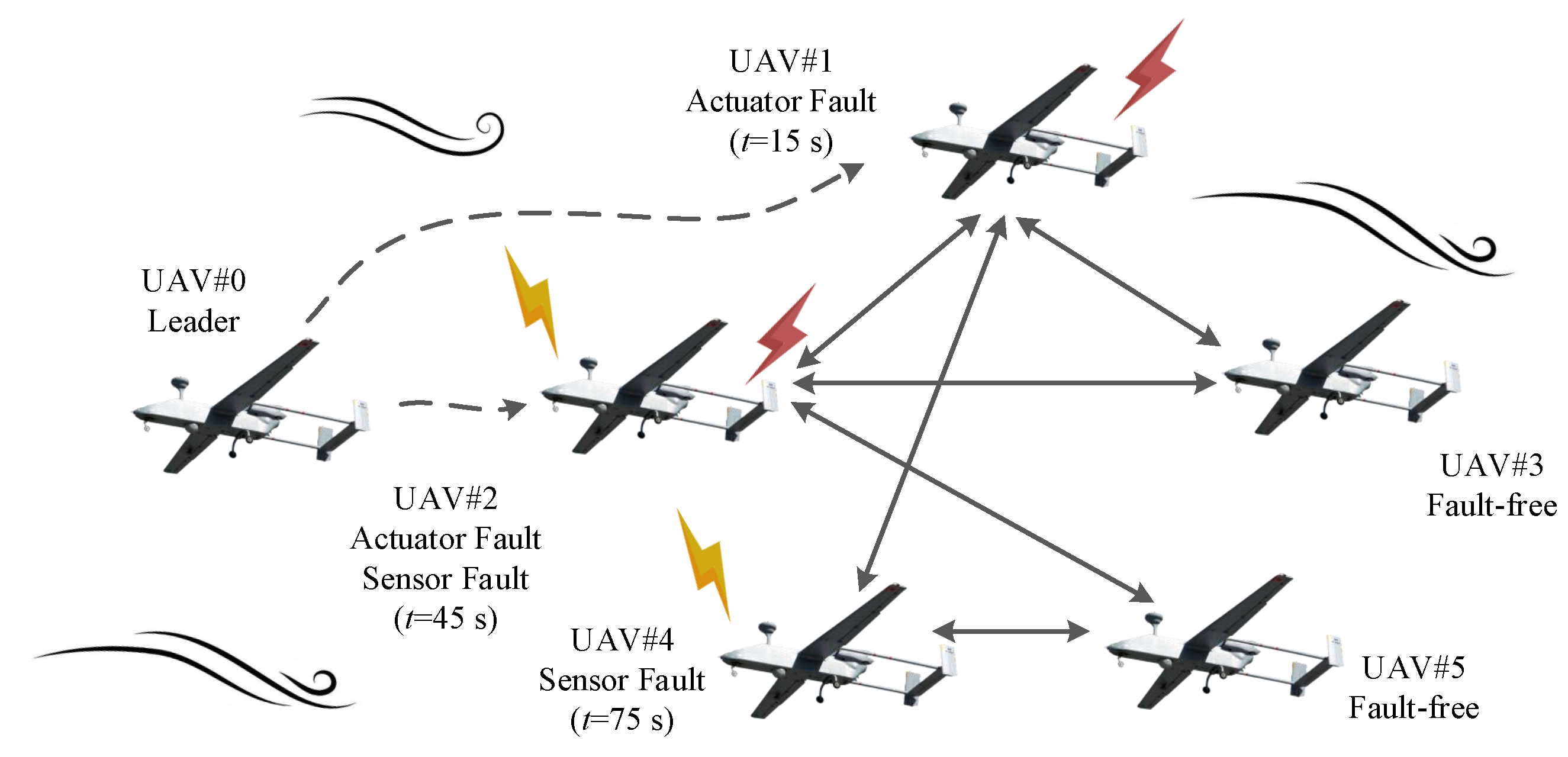
The effectiveness of the designed FD and FTCC scheme was verified by means of simulations described in this section. The structure and aerodynamic parameters of fixed-wing UAVs referred to [42]. In the simulations, actuator faults were encountered by UAV # 1  at  t = 15  s and by UAV # 2  at  t = 45  s, respectively. Sensor faults were encountered by UAV # 2  at  t = 40  s and by UAV # 4  at  t = 75  s, respectively. The actuator and sensor faults are given in Table 1. Wind disturbances were encountered by the UAVs at  t = 10  s in the simulations,  W y = 0 W z = 0 , and  W x  are given in Table 2.
The chosen design control parameters were  T m a x = 100 η 2 I = diag { 0.6 , 0.6 , 0.6 } k b = 0.5 x ̲ 2 i 1 = 0 x ¯ 2 i 1 = 32 x ̲ 2 i 2 = 0.2 x ¯ 2 i 2 = 0.2 x ̲ 2 i 3 = 0.2 x ¯ 2 i 3 = 0.2 p i = 0.95 q i = 1.2 s 1 i = 1.9 s 2 i = 2.4 K 2 i = diag { 15 , 23 , 23 } K 3 i = diag { 10 , 22 , 22 } K 4 i = diag { 33 , 3 , 3 } K 5 i = diag { 36 , 3 , 3 } . The parameters for UIOs are designed as  a 1 = 0.65 b 1 = 0.85 a 3 = 0.55 b 3 = 0.75 L 1 = L 2 = 32 L 3 = 5 L 4 = 6 L 5 = 15 L 6 = 16 . The parameter for FD was designed as  H 1 i = 3 . The initial conditions of fixed-wing UAVs were  x 10 ( 0 ) = [ 0 , 0 , 0 ] T  m,  x 11 ( 0 ) = [ 0 , 0.01 , 1030 ] T  m,  x 12 ( 0 ) = [ 0.02 , 27 , 1012 ] T  m,  x 13 ( 0 ) = [ 0.02 , 27 , 1012 ] T  m,  x 14 ( 0 ) = [ 0.01 , 18 , 976 ] T  m,  x 15 ( 0 ) = [ 0.01 , 18 , 976 ] T  m,  V i ( 0 ) = 30 m / s γ i ( 0 ) = 0 χ i ( 0 ) = 0 . The expected value of the relative position between fixed-wing UAVs are shown in Table 3. The trajectory of the leader was given by  x 10  = [30t , 0 , 1000 ] T  m. The communication topology of the UAVs is shown in Figure 2. Thus, the Laplacian matrix and leader adjacency matrix could be calculated as: L = D A = 0 1 1 1 0 1 0 1 0 1 1 1 0 0 0 1 0 0 0 1 0 1 0 1 0 3 0 0 0 0 0 3 0 0 0 0 0 2 0 0 0 0 0 2 0 0 0 0 0 2 = 3 1 1 1 0 1 3 1 0 1 1 1 2 0 0 1 0 0 2 1 0 1 0 1 2 , C = 1 0 0 0 0 0 1 0 0 0 0 0 0 0 0 0 0 0 0 0 0 0 0 0 0 .
Solving the matrix inequality (30) by means of the LMI toolbox, matrices  P 1  and  P 2  could be calculated as: P 1 = 10 2 1.56 0 0 0 0 1.56 0 0 0 0 0.49 2.41 0 0 2.41 3.78 , P 2 = 10 2 0.25 0 0 0.23 0 0.26 0 0 0 0 0.26 0 0.23 0 0 6.03
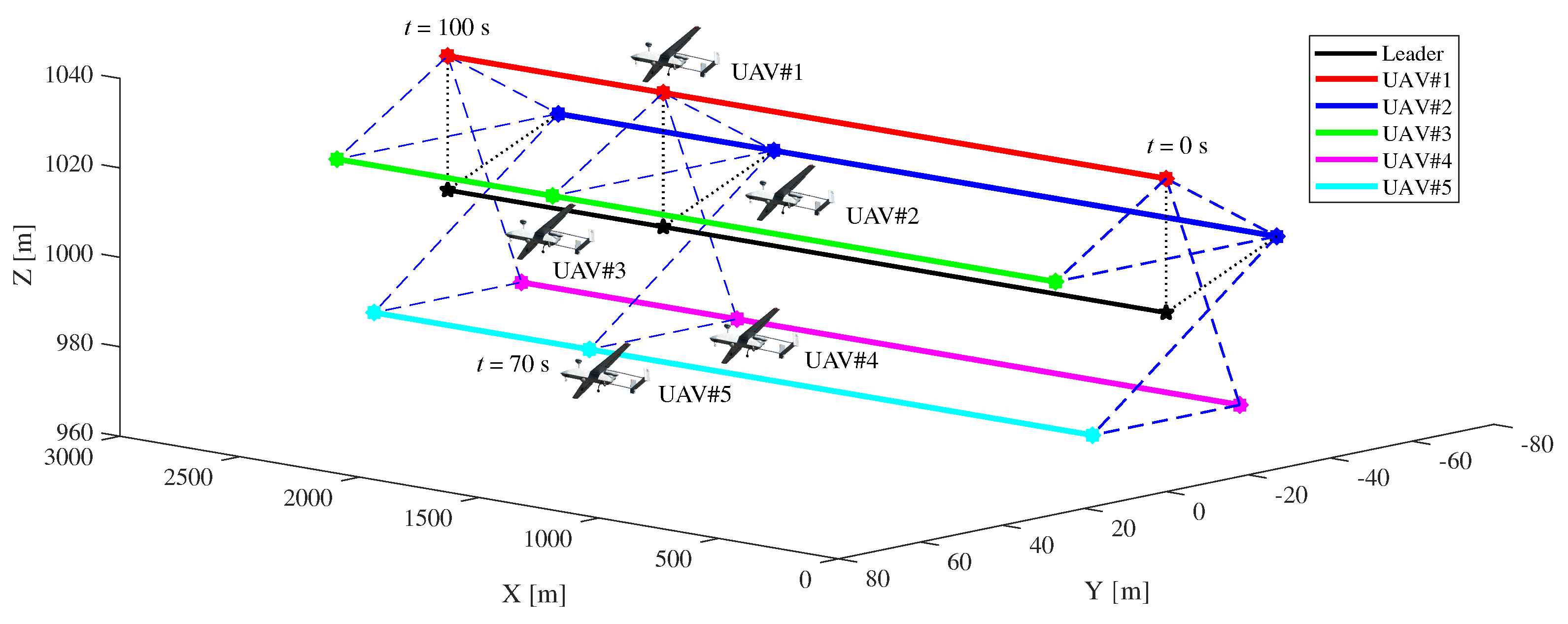
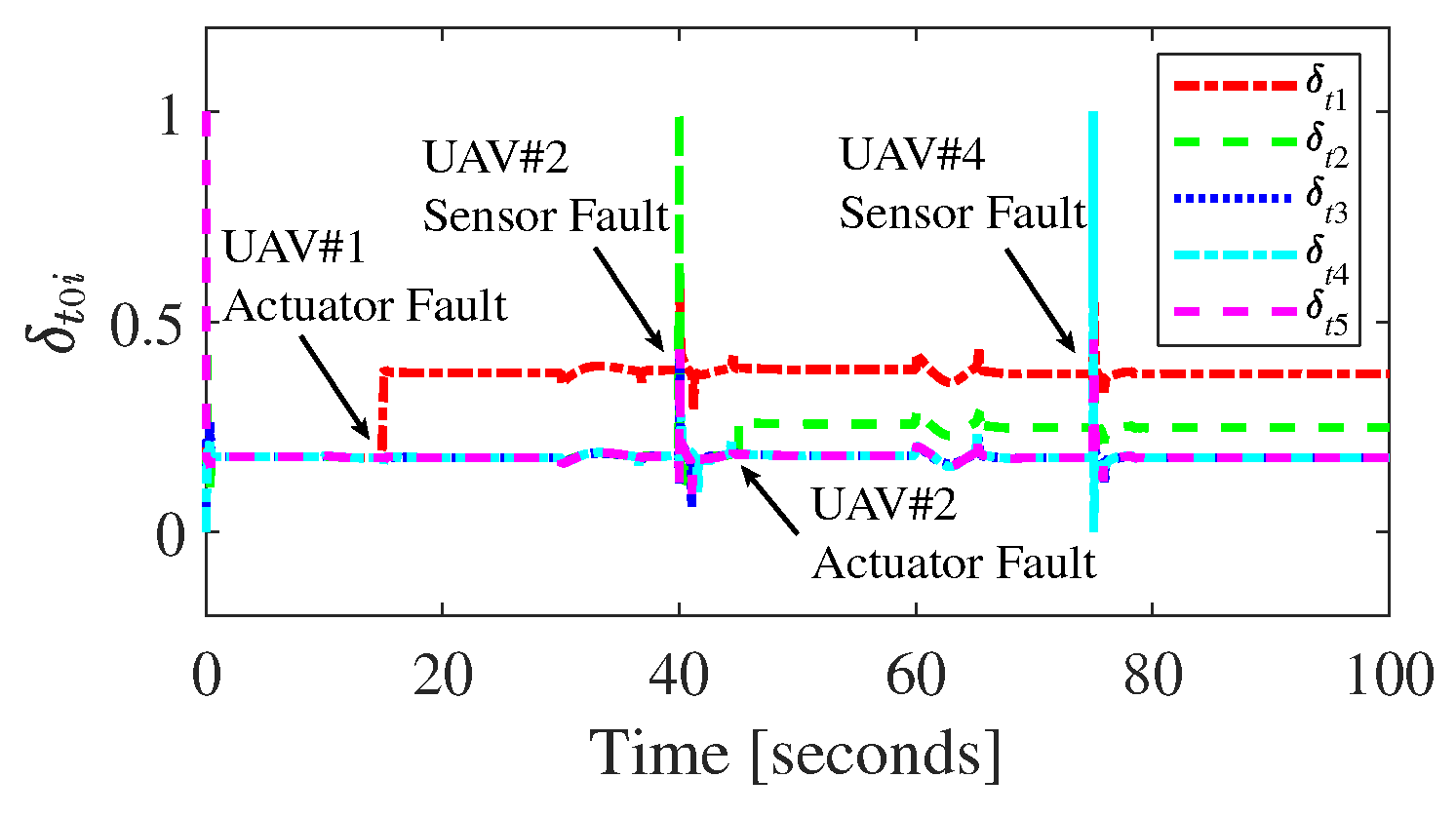
Figure 3 illustrates the flight paths of multi-UAVs. It can be seen that the fixed-wing UAVs kept cooperative formation flight even if the multi-UAV system was subjected to actuator faults, sensor faults, and wind disturbances. The thrust throttle setting of UAV # i  ( i = 1 , 2 , 3 , 4 , 5 )  is presented in Figure 4. The control inputs enabled a quick response as the faults and disturbances were encountered. 
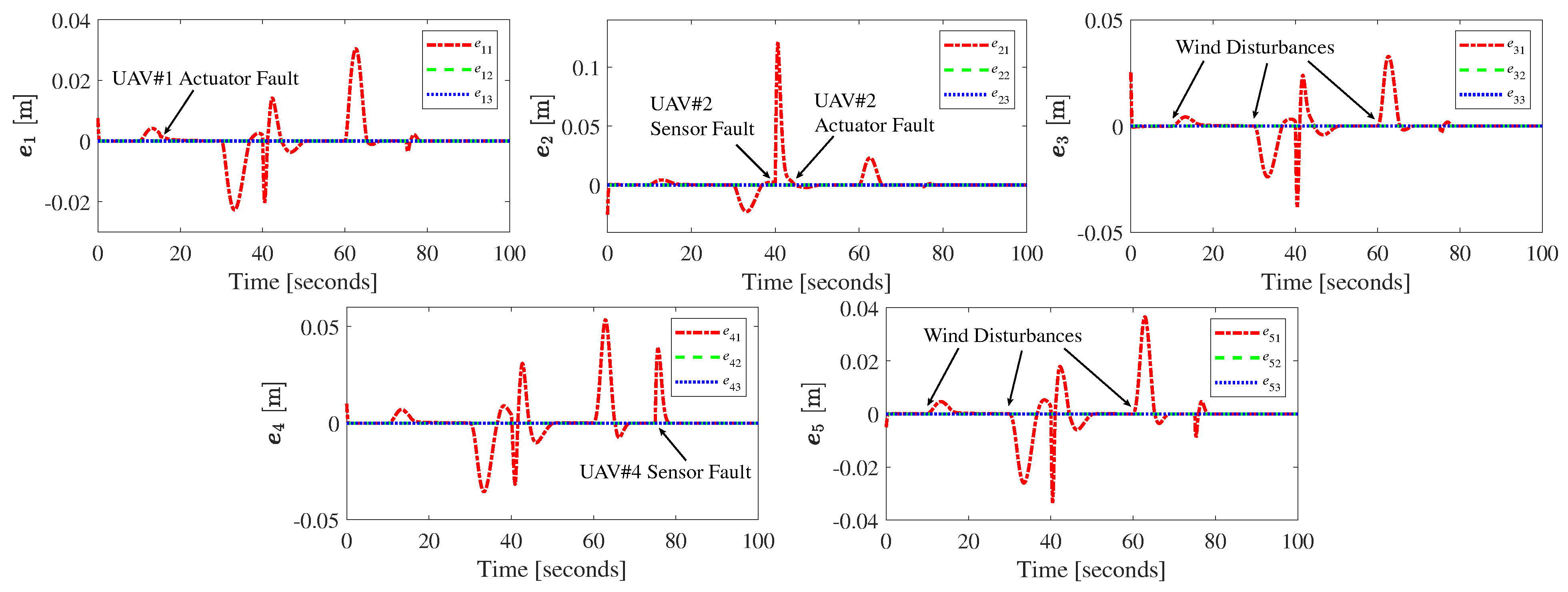
Figure 5 demonstrates the generalized position tracking errors of the ith UAV, and it can be observed that the errors were convergent to a neighborhood containing zero. 
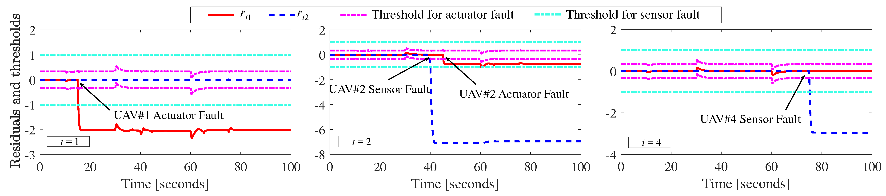
Figure 6 shows the residuals and thresholds of UAV # 1 , 2 , 4  
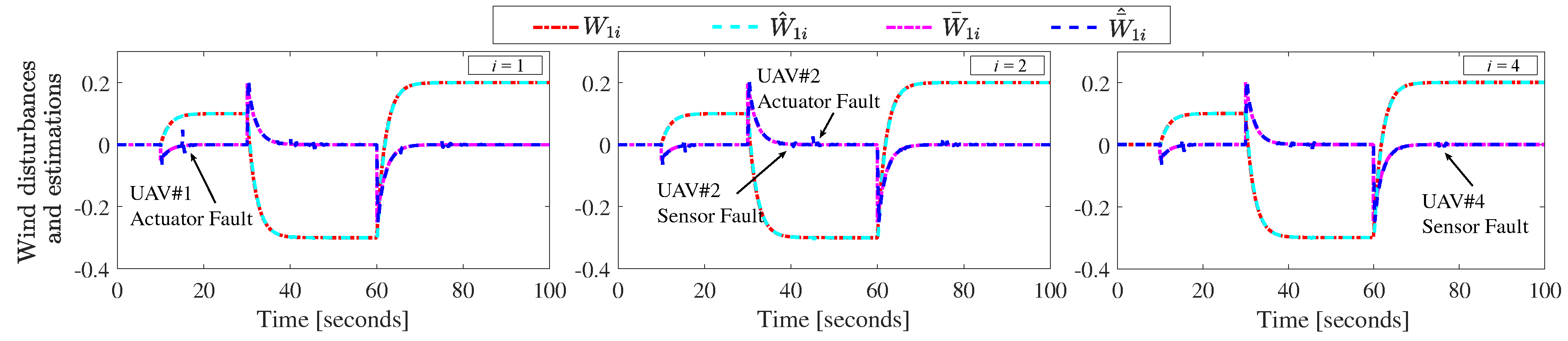
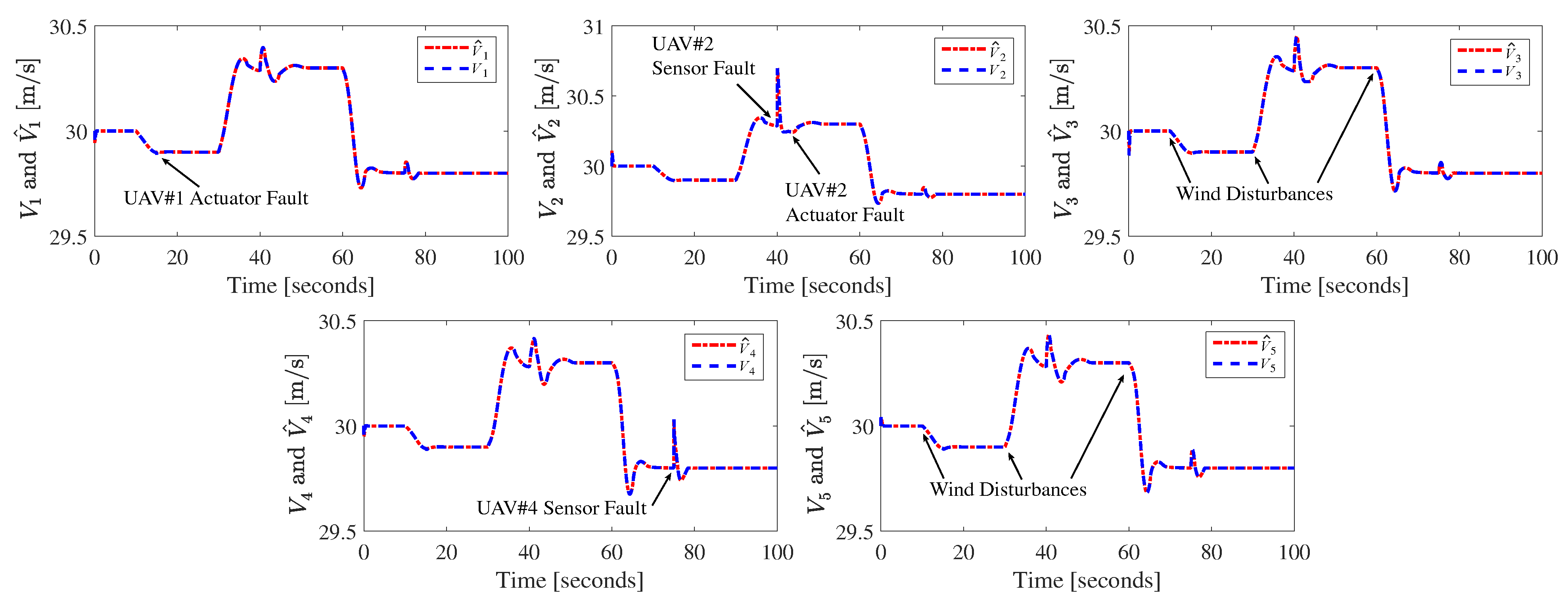
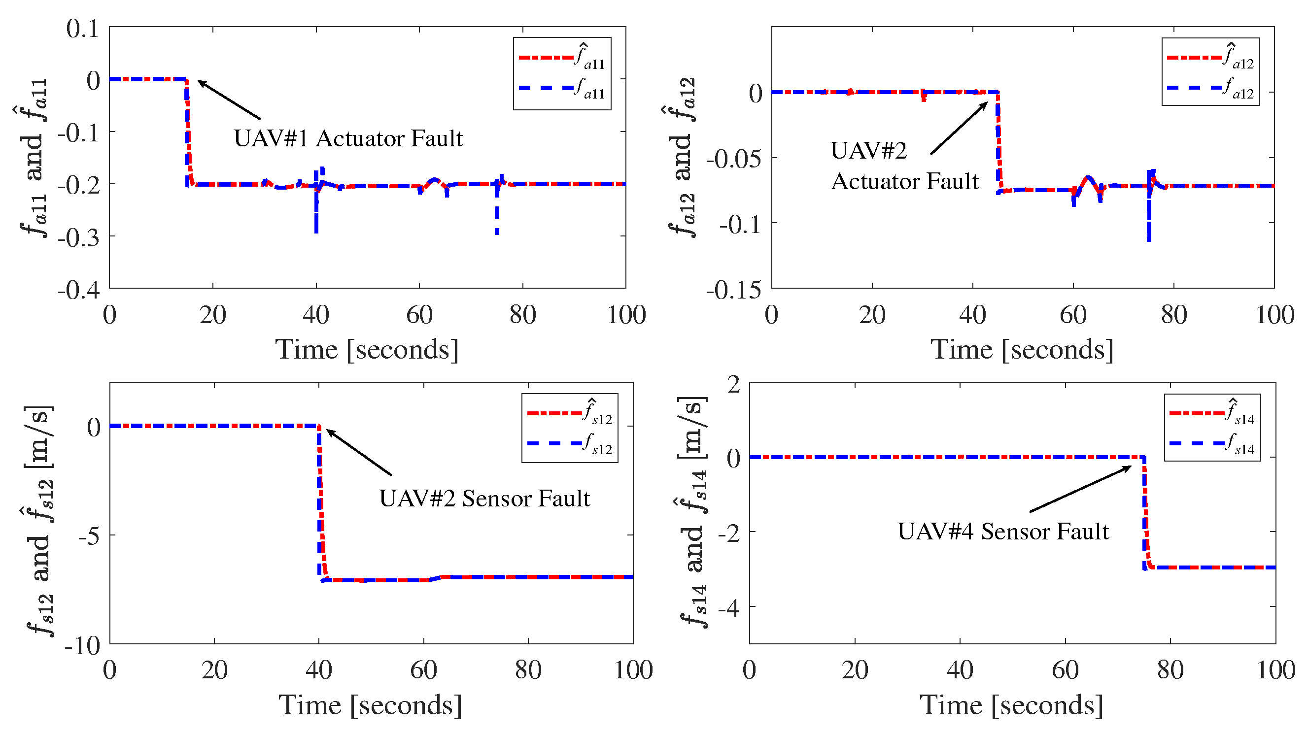
for the FD unit, respectively. It can be seen from the FD results that the residual functions for actuator fault and sensor fault exceeded the corresponding FD thresholds when an actuator fault or a sensor fault occurred. Meanwhile, the residual signals were smaller than the corresponding FD thresholds if no faults occurred. Therefore, the occurrence of actuator and sensor faults could be promptly detected by utilizing the designed FD scheme. The estimations of wind disturbances, airspeed, and faults are demonstrated in Figure 7, Figure 8, and Figure 9, respectively. It can be observed that the developed cooperative UIOs had excellent observation capabilities. The states of the multi-UAV system, disturbances, and faults approximated rapidly and accurately. Furthermore, it was found from the above simulation results that the flight performance of UAVs was affected if neighboring UAVs sufferred from faults.
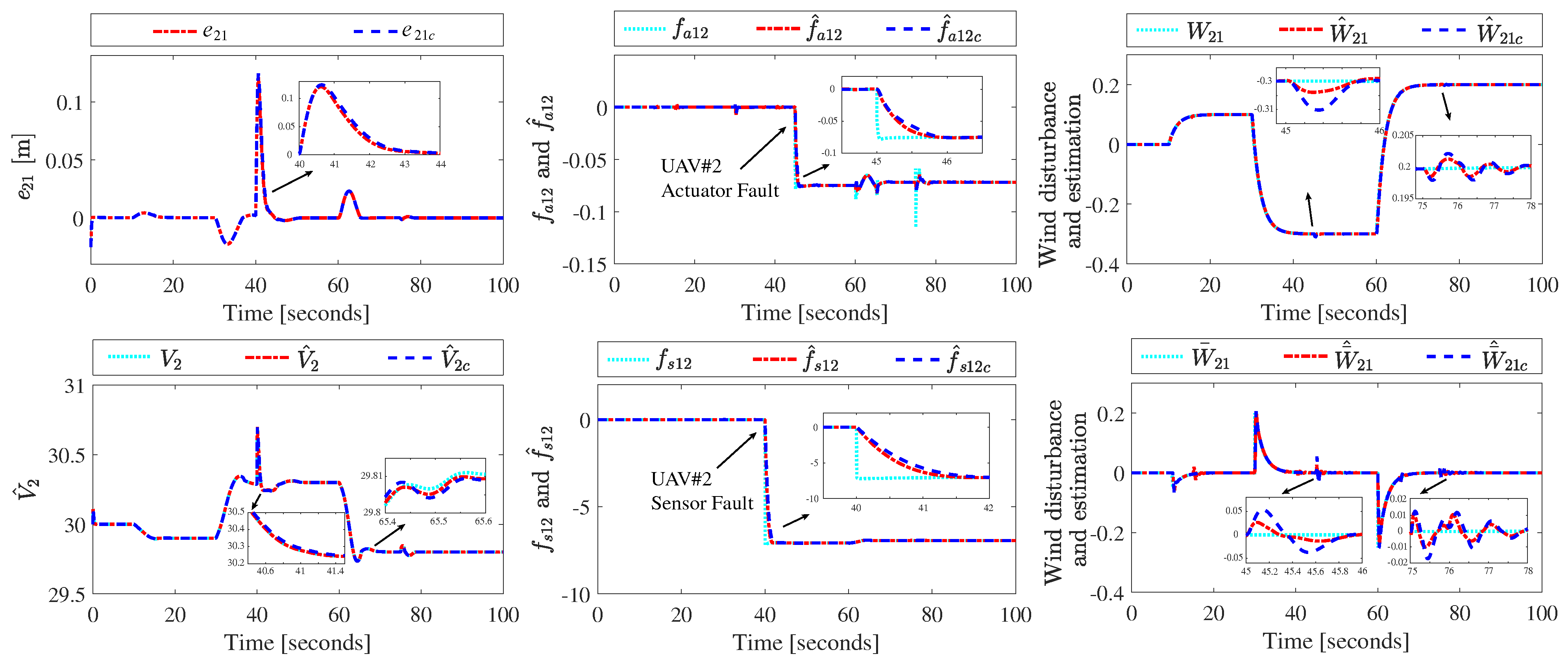
The comparative simulations between the proposed cooperative FD scheme and the individual FD scheme demonstrated the superiority of the proposed scheme. Note that the comparative individual FD scheme was derived by removing cooperative terms, including  φ 1 i  and  φ 2 i  from the UIOs. Consider the fact that UAV # 2  simultaneously encountered actuator and sensor faults, only the generalized position tracking error and estimations of the velocity, faults, and wind disturbances of UAV # 2  are presented to show the superiority of the developed method. It can be seen from Figure 10 that the convergence rate of tracking errors under the developed method was faster than the comparative scheme. Therefore, one can conclude that the performance of the developed FD scheme is enhanced by introducing cooperative terms.

6. Conclusion and Future Work

In this study, the FD and FTCC schemes were propounded for multiple fixed-wing UAVs against actuator faults, sensor faults, and wind disturbances. In the FD unit, the faulty UAV model with wind disturbances was linearized and the system was converted into two subsystems by using state and output transformations. Then, cooperative UIOs were developed to estimate the states, faults, and disturbances. The adaptive thresholds were designed to detect actuator and sensor faults by using the observers’ estimations. In the FTCC unit, state constraints were considered. Furthermore, backstepping-based fixed-time FTCC laws were proposed for multi-UAVs suffering from actuator faults, sensor faults, and wind disturbances. Lyapunov analysis proved the fixed-time convergence of the tracking errors in the multi-UAV system. The simulation results showed the effectiveness of the FD and FTCC strategies.
In the current study, only the effectiveness loss, deviation of thrust throttle setting, and pitot faults were considered in the FD and FTCC scheme design for the fixed-wing follower UAVs. As one of future works, more actuator and sensor faults, such as actuator stuck faults, will be investigated. Furthermore, the effects of faults and wind disturbances on real UAV testbeds with one leader UAV, or even multiple leader UAVs, will be considered in future research. Eventually, implementation and experimental tests of the proposed scheme on systems with real UAVs will be carried out.

Author Contributions

Conceptualization, Y.C., G.X. and Y.Z.; Methodology, Z.Y. (Zhongyu Yang) and M.L.; Supervision, Z.Y. (Ziquan Yu) and G.X.; Validation, Z.Y. (Zhongyu Yang) and M.L.; Visualization, Z.Y. (Zhongyu Yang); Writing—original draft, Z.Y. (Zhongyu Yang); Writing—review & editing, Z.Y. (Ziquan Yu), Y.C. and Y.Z. All authors have read and agreed to the published version of the manuscript.

Funding

This work was supported in part by the National Natural Science Foundation of China (No. 62003162, 61833013, 62233009), the Natural Science Foundation of Jiangsu Province of China (No. BK20200416, BK20222012), the China Postdoctoral Science Foundation (No. 2020TQ0151, 2020M681590), the Industry–University Research Innovation Foundation for the Chinese Ministry of Education (No. 2021ZYA02005), the Science and Technology on Space Intelligent Control Laboratory (No. HTKJ2022KL502015), the Aeronautical Science Foundation of China (No. 20220007052003, 20200007018001), the Postgraduate Research & Practice Innovation Program of NUAA (No. xcxjh20220325); and the Natural Sciences and Engineering Research Council of Canada.

Data Availability Statement

The data presented in this study are available on request from the corresponding author upon reasonable request.

Conflicts of Interest

The authors declare no conflict of interest.

References

  1. Yang, X.S.; Tang, L.B.; Wang, H.S.; He, X.X. Early detection of forest fire based on unmaned aerial vehicle platform. In Proceedings of the IEEE International Conference on Signal, Information and Data Processing, Chongqing, China, 11–13 December 2019. [Google Scholar]
  2. Yfantis, E.A. A UAV with autonomy, pattern recognition for forest fire prevention, and AI for providing advice to firefighters fighting forest fires. In Proceedings of the IEEE 9th Annual Computing and Communication Workshop and Conference, Las Vegas, NV, USA, 7–9 January 2019. [Google Scholar]
  3. Bi, J.T.; Mao, W.B.; Gong, Y.J. Research on image mosaic method of UAV image of earthquake emergency. In Proceedings of the International Conference on Agro-Geoinformatics, Beijing, China, 11–14 August 2014. [Google Scholar]
  4. Li, Z.R.; Liu, Y.; Walker, R.; Hayward, R.; Zhang, J.L. Towards automatic power line detection for a UAV surveillance system using pulse coupled neural filter and an improved Hough transform. Mach. Vis. Appl. 2010, 21, 677–686. [Google Scholar] [CrossRef] [Green Version]
  5. Hristov, G.; Raychev, J.; Kinaneva, D.; Zahariev, P. Emerging methods for early detection of forest fires using unmanned aerial vehicles and lorawan sensor networks. In Proceedings of the 28th EAEEIE Annual Conference, Hafnarfjordur, Iceland, 26–28 September 2018. [Google Scholar]
  6. Fahmani, L.; Garfaf, J.; Boukhdir, K.; Benhadou, S.; Medromi, H. Unmanned aerial vehicles inspection for overhead high voltage transmission lines. In Proceedings of the International Conference on Innovative Research in Applied Science, Engineering and Technology, Meknes, Morocco, 16–19 April 2020. [Google Scholar]
  7. Wu, G.F.; Gao, X.G.; Fu, X.W.; Wan, K.F.; Di, R.H. Mobility control of unmanned aerial vehicle as communication relay in airborne multi-user systems. Chin. J. Aeronaut. 2019, 32, 1520–1529. [Google Scholar] [CrossRef]
  8. Peng, H.; Shen, L.C.; Zhu, H.Y. Multiple UAV cooperative area search based on distributed model predictive control. Acta Aeronaut. Astronaut. Sin. 2010, 31, 593–601. [Google Scholar]
  9. No, T.S.; Kim, Y.D.; Tahk, M.J.; Jeon, G.E. Cascade-type guidance law design for multiple-UAV formation keeping. Aerosp. Sci. Technol. 2011, 15, 431–439. [Google Scholar] [CrossRef]
  10. Seo, J.B.; Kim, Y.D.; Tsourdos, A.; White, B.A. Multiple UAV formation reconfiguration with collision avoidance guidance via differential geometry concept. In Proceedings of the International Congress of the Aeronautical Sciences ICAS, Brisbane, Australia, 23–28 September 2012; pp. 1–8. [Google Scholar]
  11. Bai, R.G.; Sun, X.; Chen, Q.S.; Quan, X.W. Multiple UAV cooperative trajectory planning based on Gauss pseudospectral method. J. Astronaut. 2014, 35, 1022–1029. [Google Scholar]
  12. Yu, Z.Q.; Zhang, Y.M.; Qu, Y.H. Prescribed performance-based distributed fault-tolerant cooperative control for multi-UAVs. Trans. Inst. Meas. Control 2019, 41, 975–989. [Google Scholar] [CrossRef]
  13. Chi, C.Z.; Su, L.; Lyu, Y.X.; Shi, J.P.; Huang, S. Research on real-time fault detection of UAV flight control system sensor based on Riemannian manifold. In Advances in Guidance, Navigation and Control: Proceedings of 2022 International Conference on Guidance, Navigation and Control, Harbin, China, 5–7 August 2022; Springer: Berlin/Heidelberg, Germany, 2023; pp. 1219–1227. [Google Scholar]
  14. Grehan, J.; Ignatyev, D.; Zolotas, A. Fault detection in aircraft flight control actuators using support vector machines. Machines 2023, 11, 211. [Google Scholar] [CrossRef]
  15. Al-Haddad, L.A.; Jaber, A.A. An intelligent fault diagnosis approach for multirotor UAVs based on deep neural network of multi-resolution transform features. Drones 2023, 7, 82. [Google Scholar] [CrossRef]
  16. Liu, Z.B.; Wang, L.N.; Song, Y.C.; Dang, Q.Q.; Ma, B.D. Fault diagnosis and accommodation for multi-actuator faults of a fixed-wing unmanned aerial vehicle. Meas. Sci. Technol. 2022, 33, 075903. [Google Scholar] [CrossRef]
  17. Zhang, J.; Swain, A.K.; Nguang, S.K. Robust sensor fault estimation scheme for satellite attitude control systems. J. Frankl. Inst. 2013, 350, 2581–2604. [Google Scholar] [CrossRef]
  18. Wu, Y.K.; Jiang, B.; Lu, N.Y.; Yang, H.; Zhou, Y. Multiple incipient sensor faults diagnosis with application to high-speed railway traction devices. ISA Trans. 2017, 67, 183–192. [Google Scholar] [CrossRef]
  19. Yin, S.; Gao, H.J.; Qiu, J.B.; Kaynak, O. Descriptor reduced-order sliding mode observers design for switched systems with sensor and actuator faults. Automatica 2017, 76, 282–292. [Google Scholar] [CrossRef]
  20. Atallah, M.; Okasha, M.; Dief, T.N.; Jallad, A.H. Optimal consensus control for multi-satellite assembly in elliptic orbit with input saturation. Acta Astronaut. 2023, 208, 82–90. [Google Scholar] [CrossRef]
  21. Yu, Y.S.; Shi, C.B.B.; Shan, D.; Lippiello, V.; Yang, Y. A hierarchical control scheme for multiple aerial vehicle transportation systems with uncertainties and state/input constraints. Appl. Math. Model. 2022, 109, 651–678. [Google Scholar] [CrossRef]
  22. Chen, Q.J.; Jin, Y.Q.; Wang, T.Y.; Wang, Y.; Yan, T.L.; Long, Y.F. UAV formation control under communication constraints based on distributed model predictive control. IEEE Access 2022, 10, 126494–126507. [Google Scholar] [CrossRef]
  23. Aliyari, M.; Wong, W.K.; Bouteraa, Y.; Najafinia, S.; Fekih, A.; Mobayen, S. Design and implementation of a constrained model predictive control approach for unmanned aerial vehicles. IEEE Access 2022, 10, 91750–91762. [Google Scholar] [CrossRef]
  24. Yan, K.; Wu, Q.X. Adaptive tracking flight control for unmanned autonomous helicopter with full state constraints and actuator faults. ISA Trans. 2022, 128, 32–46. [Google Scholar] [CrossRef]
  25. Wang, Z.X.; Yang, P.; Hu, X.K.; Zhang, Z.Q.; Wen, C.W. Sliding mode fault tolerant control of quadrotor UAV with state constraints under actuator fault. Int. J. Innov. Comput. I 2021, 17, 639–653. [Google Scholar]
  26. Zhang, B.Y.; Sun, X.X.; Lv, M.L.; Liu, S.G.; Li, L. Distributed adaptive fixed-time fault-tolerant control for multiple 6-DOF UAVs with full-state constraints guarantee. IEEE Syst. J. 2021, 16, 4792–4803. [Google Scholar] [CrossRef]
  27. Li, Z.; Chen, X.; Xie, M.Y.; Zhao, Z.H. Adaptive fault-tolerant tracking control of flying-wing unmanned aerial vehicle with system input saturation and state constraints. Trans. Inst. Meas. Control 2022, 44, 880–891. [Google Scholar] [CrossRef]
  28. Zhou, Y.; Dong, W.H.; Liu, Z.C.; Lv, M.L.; Zhang, W.Q.; Chen, Y. IBLF-based fixed-time fault-tolerant control for fixed-wing UAV with guaranteed time-varying state constraints. IEEE Trans. Veh. Technol. 2022, 72, 4252–4266. [Google Scholar] [CrossRef]
  29. Jin, X. Fault tolerant finite-time leader–follower formation control for autonomous surface vessels with LOS range and angle constraints. Automatica 2016, 68, 228–236. [Google Scholar] [CrossRef]
  30. Li, J.Q.; Kumar, K.D. Fault tolerant attitude synchronization control during formation flying. J. Aerosp. Eng. 2011, 24, 251–263. [Google Scholar] [CrossRef]
  31. Zhang, J.X.; Yang, G.H. Fault-tolerant leader-follower formation control of marine surface vessels with unknown dynamics and actuator faults. Int. J. Robust Nonlinear Control 2018, 28, 4188–4208. [Google Scholar] [CrossRef]
  32. Cui, B.; Zhao, C.H.; Ma, T.D.; Feng, C. Distributed adaptive neural network control for a class of heterogeneous nonlinear multi-agent systems subject to actuation failures. Int. J. Syst. Sci. 2017, 48, 559–570. [Google Scholar] [CrossRef]
  33. Zhou, N.; Xia, Y.Q. Distributed fault-tolerant control design for spacecraft finite-time attitude synchronization. Int. J. Robust Nonlinear Control 2016, 26, 2994–3017. [Google Scholar] [CrossRef]
  34. Yu, Z.Q.; Zhang, Y.M.; Liu, Z.X.; Qu, Y.H.; Su, C.Y. Distributed adaptive fractional-order fault-tolerant cooperative control of networked unmanned aerial vehicles via fuzzy neural networks. IET Contr. Theory Appl. 2019, 13, 2917–2929. [Google Scholar] [CrossRef]
  35. Wu, Z.H.; Zheng, S.P. Fixed-time fault-tolerant tracking control of fixed-wing UAVs with actuator fault and unmatched disturbances. Int. J. Aerosp. Eng. 2022, 2022, 6447812. [Google Scholar] [CrossRef]
  36. Han, B.; Jiang, J.; Yu, C.J.; Cao, T. Distributed fault estimation and fixed-time fault-tolerant formation control for multi-UAVs subject to sensor faults. J. Intell. Robot. Syst. 2022, 105, 80. [Google Scholar] [CrossRef]
  37. Yu, Z.Q.; Zhang, Y.M.; Jiang, B.; Su, C.Y.; Fu, J.; Jin, Y.; Chai, T.Y. Fractional-order adaptive fault-tolerant synchronization tracking control of networked fixed-wing UAVs against actuator-sensor faults via intelligent learning mechanism. IEEE Trans. Neural Netw. Learn. Syst. 2021, 32, 5539–5553. [Google Scholar] [CrossRef]
  38. Shao, S.Y.; Chen, M.; Shi, P. Robust Discrete-Time Flight Control of UAV with External Disturbances; Springer: Berlin/Heidelberg, Germany, 2021; Volume 317. [Google Scholar]
  39. Cui, G.Z.; Yang, W.; Yu, J.P.; Li, Z.; Tao, C.B. Fixed-time prescribed performance adaptive trajectory tracking control for a QUAV. IEEE T. Circuits-II 2021, 69, 494–498. [Google Scholar] [CrossRef]
  40. Yan, X.G.; Edwards, C. Sensor fault detection and isolation for nonlinear systems based on a sliding mode observer. Int. J. Adapt. Control Signal Process. 2007, 21, 657–673. [Google Scholar] [CrossRef] [Green Version]
  41. Lv, M.L.; Yu, W.W.; Cao, J.D.; Baldi, S. Consensus in high-power multiagent systems with mixed unknown control directions via hybrid nussbaum-based control. IEEE T. Cybern. 2020, 52, 5184–5196. [Google Scholar] [CrossRef]
  42. Lin, W. Distributed UAV formation control using differential game approach. Aerosp. Sci. Technol. 2014, 35, 54–62. [Google Scholar] [CrossRef]
Figure 1. Overall FD and FTCC scheme.
Drones 07 00503 g001
Figure 2. Communication topology.
Drones 07 00503 g002
Figure 3. Flight paths of multi-UAVs.
Drones 07 00503 g003
Figure 4. δ t 0 i  of the ith UAV.
Drones 07 00503 g004
Figure 5. The generalized position tracking errors of the ith UAV.
Drones 07 00503 g005
Figure 6. Residuals and thresholds for FD.
Drones 07 00503 g006
Figure 7. Wind disturbances and estimations.
Drones 07 00503 g007
Figure 8. Airspeeds and estimations.
Drones 07 00503 g008
Figure 9. Faults and estimations.
Drones 07 00503 g009
Figure 10. Comparison between the proposed cooperative FD scheme and the individual FD scheme.
Drones 07 00503 g010
Table 1. Description of sensor and actuator fault models.
UAV # 1 UAV # 2 UAV # 4
Actuator fault   ρ t 1 = 1 , δ t b 1 = 0 , t < 15 s ρ t 1 = 0.6 , δ t b 1 = 0.05 , t 15 s   ρ t 2 = 1 , δ t b 2 = 0 , t < 45 s ρ t 2 = 0.65 , δ t b 2 = 0.015 , t 45 s
Sensor fault   ϱ v 2 = 1 , V b 2 = 0 , t < 40 s ϱ v 2 = 0.7 , V b 2 = 20 , t 40 s   ϱ v 4 = 1 , V b 4 = 0 , t < 75 s ϱ v 4 = 0.8 , V b 4 = 3 , t 75 s
Table 2. Description of wind disturbance model.
  t < 10 s   10 s t < 30 s   30 s t < 60 s   t 60 s
  W x 0   0.1 e 0.5 t 10 + 0.1   0.4 e 0.5 t 30 0.3   0.5 e 0.5 t 60 + 0.2
Table 3. Expected value of the relative position between fixed-wing UAVs.
UAV # 1   ( i = 1 ) UAV # 2   ( i = 2 ) UAV # 3   ( i = 3 ) UAV # 4   ( i = 4 ) UAV # 5   ( i = 5 )
R i 0  [m]   [ 0 , 0 , 30 ] T   [ 0 , 27 , 12 ] T
R i 1  [m]   [ 0 , 27 , 18 ] T   [ 0 , 27 , 18 ] T   [ 0 , 18 , 54 ] T
R i 2  [m]   [ 0 , 27 , 18 ] T   [ 0 , 54 , 0 ] T   [ 0 , 45 , 36 ] T
R i 3  [m]   [ 0 , 27 , 18 ] T   [ 0 , 54 , 0 ] T
R i 4  [m]   [ 0 , 18 , 54 ] T   [ 0 , 36 , 0 ] T
R i 5  [m]   [ 0 , 45 , 36 ] T   [ 0 , 36 , 0 ] T
Disclaimer/Publisher’s Note: The statements, opinions and data contained in all publications are solely those of the individual author(s) and contributor(s) and not of MDPI and/or the editor(s). MDPI and/or the editor(s) disclaim responsibility for any injury to people or property resulting from any ideas, methods, instructions or products referred to in the content.

