Article

Performance Analysis of Multi-Hop Flying Mesh Network Using Directional Antenna Based on β-GPP

1
College of Communication Engineering, Army Engineering University of PLA, Nanjing 210007, China
2
The 63rd Research Institute, National University of Defense Technology, Nanjing 210007, China
*
Author to whom correspondence should be addressed.
Drones 2023, 7(5), 335; https://doi.org/10.3390/drones7050335
Submission received: 18 April 2023 / Revised: 16 May 2023 / Accepted: 19 May 2023 / Published: 22 May 2023
(This article belongs to the Special Issue Wireless Networks and UAV)

Abstract

:
Maintaining high system performance is critical for a multi-hop flying mesh network (FlyMesh) to perform missions in different environments. Although the Poisson point process (PPP) has been widely used for the performance analysis of FlyMesh, it still has flaws in describing the spatial distribution of the UAVs since it does not restrict the minimum distance between them. The spatial deployment of FlyMesh varies depending on the environment. Considering the relevance and practicality, we modeled the multi-hop FlyMesh using the β -Ginibre point process ( β -GPP) and equipped each UAV with a directional antenna. Under the condition of the decode-and-forward protocol, we derived the connection probability and ergodic capacity of a multi-hop FlyMesh utilizing the Laplace transform of interference. Then, we calculated an approximate expression for the interference Laplace transform based on the diagonal approximation and further obtained the coverage probability. Finally, the numerical simulation results verified the correctness of the theoretical derivation, indicating that it is possible to optimize the system’s performance based on the expressions derived in this paper.

1. Introduction

Recently, unmanned aerial vehicles (UAVs) have received much attention and research due to their controlled mobility and on-demand deployment. For example, UAVs can be used as airborne wireless communication platforms, such as mobile base stations, to quickly restore communication services and ensure communication quality [1]. UAVs can also act as mobile relays to connect two or more distant users for communication [2]. As an aerial base station or mobile relay, they greatly improve the service quality of the network [3]. In addition, UAVs can be applied to mobile data collection and information dissemination to facilitate various Internet of Things (IoT) applications. Multiple UAVs are organized into a group and deployed together to achieve the coverage of an area, in which UAVs communicate with each other in a decentralized and ad hoc manner; this type of network is called a flying mesh network (FlyMesh). Directional antennas are used to improve the efficient coverage of UAVs. At the same time, they can increase the network capacity and increase the robustness of the network [4]. It is known that FlyMesh will experience frequent topological changes due to the rapid movement of UAV nodes [5]. To ensure the continuous service of FlyMesh, maintenance personnel must maintain good connections between drones. Therefore, establishing a suitable mathematical model to analyze the performance of FlyMesh is crucial.
Stochastic geometry is commonly used as a tool for modeling and analyzing the performance of FlyMesh [6]. For ease of handling, UAV locations are usually modeled as a Poisson point process (PPP) [7]. PPP only applies to networks where transmitters (jammers) are deployed in a completely unplanned manner, where each UAV is considered an independent point in space and there is no relationship between UAV locations. However, existing models are difficult to reconcile because UAVs usually keep a distance from each other to improve coverage and prevent collisions. In addition, UAVs commonly use directional antennas to reduce self-interference of signals. However, in real-world environments, the location of UAVs is carefully planned to avoid interference or to extend the coverage area. That is to say, there is a repulsion (or attraction) between UAVs, which means that the actual deployed UAV locations usually form a more regular pattern of points than PPP.
The β -Ginibre point process ( β -GPP) has received wide attention as point processes reflect repulsive forces [8]. β -GPP is repulsive and treats PPP as a particular case. In this context, β -GPP was utilized to explain the spatial regularity among UAVs in this paper. In contrast to PPP, β -GPP employs the parameter β to restrict the minimum distance between UAVs. Different deployment environments are reflected by the repulsive parameter β . GPP is similar to PPP when β 0 , and the UAVs are in a uniform distribution while β 1 . Therefore, the distribution of UAVs in a given environment can be more accurately described by the repulsive parameter β . We derived the connection probability of a multi-hop relay link by utilizing the Laplace function of the β -GPP distribution, based on the connection probability to derive the ergodic capacity of the multi-hop relay. To better describe the ability of FlyMesh to provide services, we used the approximate expression of the diagonal kernel matrix to calculate the coverage probability. Finally, numerical simulations verified the accuracy of the derived theoretical expressions. The main objective of this paper was to introduce and promote β -GPP as a UAV network model in which nodes exhibit repulsive forces. Compared with the PPP model, β -GPP not only captures the application scenarios of real networks but is also analytically easy to handle. The main contributions of our work can be summarized as follows:
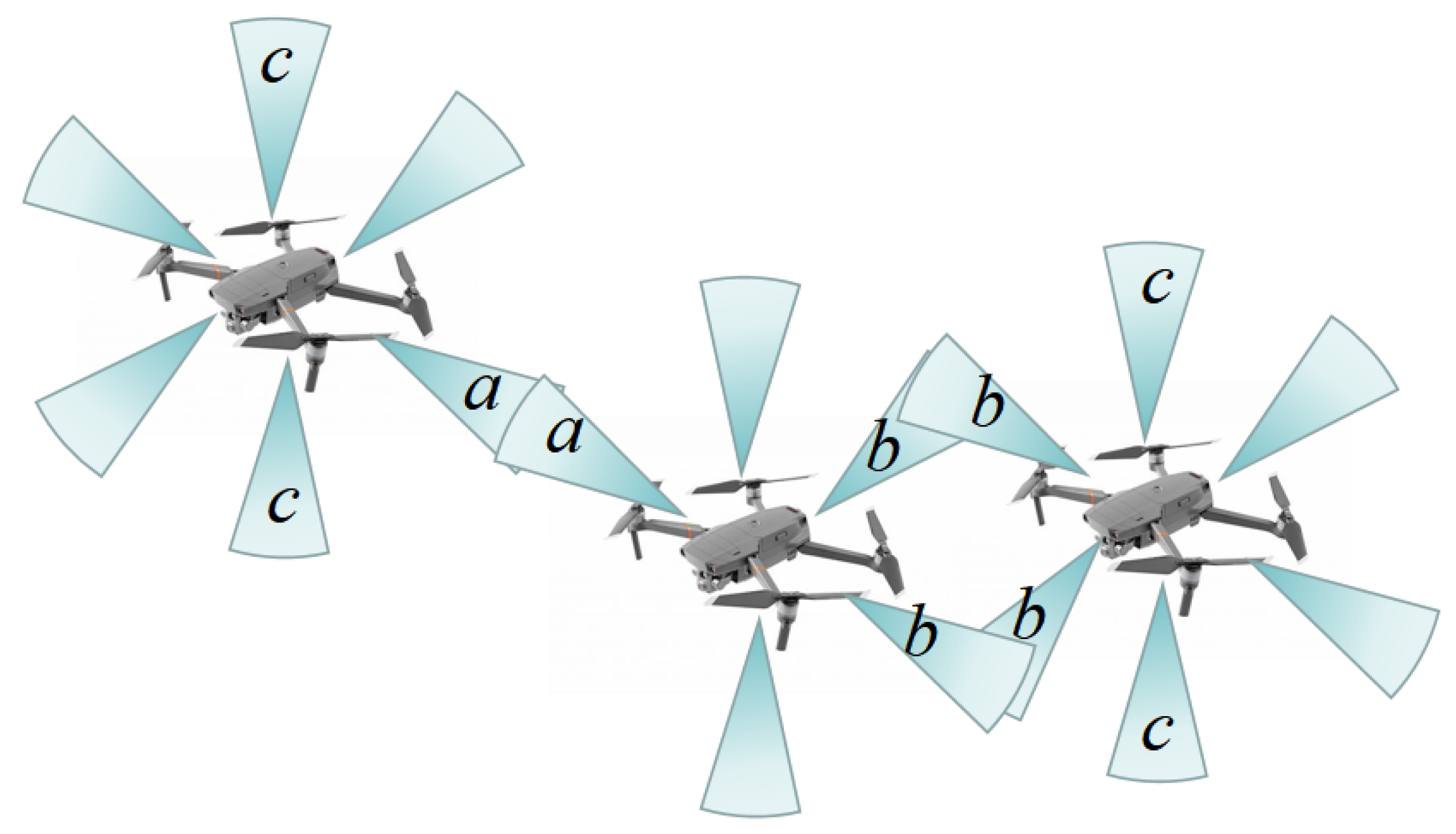
  • The spatial distribution of the UAVs was modeled as β -GPP, and the UAVs were equipped with directional antennas to reduce signal self-interference. The repulsive parameter β describes different application environments with tunability. Different values of β describe the UAVs’ deployment in different environments, which makes our model more practical;
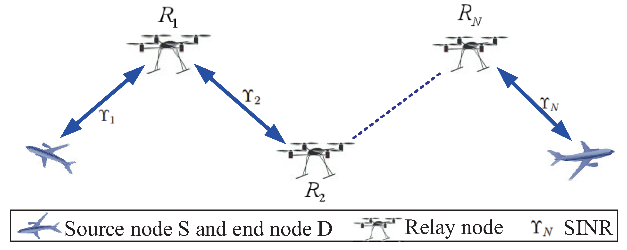
  • We considered the information transmission performance of a certain instantaneous snapshot. By ignoring small-scale fading of interfering links and using random geometry tools, an approximate expression for the coverage probability of multi hop relay systems was obtained, thereby obtaining the traversal capacity. Then, according to the diagonal approximate matrix property of β -GPP, we derived the approximate expression of the coverage probability. The above analysis results can better predict the performance of FlyMesh in different environments;
  • Based on the theoretical expressions obtained, we analyzed the effects of various parameters on the performance of FlyMesh in different environments. The simulation results verified the correctness of the theoretical expression. We also adjusted the beam width t h e t a and the number of relay hops N, to achieve the best network performance according to the repulsive parameter β .
The rest of this paper is organized as follows. Section 2 describes the related work. Section 3 briefly introduces the β -GPP related mathematics and FlyMseh system model. Section 4 gives the connection probability and ergodic capacity of multi-hop relaying, and derives an approximate expression for the coverage probability. Section 5 provides numerical results to verify the correctness of our theoretical derivation. Finally, Section 6 summarizes the work and looks forward to the application of the results.

2. Related Work

UAVs are widely utilized as low-altitude platforms owing to their effortless flexibility, inexpensive price, and simplicity of deployment [9]. Current academic research and industrial associations propose UAVs as aerial base stations and evaluate their application characteristics in various systems. For example, the authors of [10] consider UAVs to provide downlink services for network coverage in rural areas. The authors of [11] construct a UAV network that collects data from IoT devices and starts transmission whenever the IoT devices are within the coverage area of the UAV. In [12,13], radio power transmission from UAVs to end devices was proposed to improve battery life or to enable local computing. In [14], a deep reinforcement learning-based algorithm was proposed to solve the UAV trajectory planning, mission scheduling, and deployment in complex regional scenarios.
To facilitate the modeling and analysis of wireless geometric networks, PPP is widely used because of its ease of handling. In most of the research on stochastic FlyMesh, PPP is usually used to model the spatial distribution of UAVs. In [15], a 3D wireless network of UAVs was modeled as a multilayer network with the location of UAVs at each layer following the PPP model, which was derived analytically in addition to the 3D UAVs switching probability. Reference [16] derived the coverage performance of the UAV-assisted millimeter-wave cellular network using the PPP model and analyzed the optimal key parameters to maximize the coverage probability. Although the PPP model provides many useful theoretical results for our UAV network analysis, it has certain drawbacks due to the independence of the described UAVs’ location distribution.
Therefore, a better point process must be considered to capture the deployment of UAVs in real-world environments. β -GPP had received much attention as describing a point process with repulsive power, where 0 < β < 1 , describing the strength of repulsion between points. In contrast, GPP belongs to a class of deterministic point processes (DPP) [17]. β -GPP falls between GPP and PPP, and it is more regular than PPP and treats PPP as a particular case. Therefore, β -GPP was a soft-core model with a scaling function according to the variation of the repulsive parameter β . In [18], an ambient radio frequency energy harvesting wireless sensor network was considered, where the location of the ambient radio frequency source was modeled as a β -GPP and the average value of energy, outage probability, and transmission interruption probability were harvested by the Laplace transform of β -GPP. In [19], the performance of a specific clustered network with a wireless node distribution location modeled as β -GPP was investigated and its approximate expressions were obtained by approximating the simplified palm distribution of β -GPP as an inhomogeneous Poisson point process (IPPP). On this basis, the approximate expressions for the message outage probability, the overall outage probability, and the transmission capacity were obtained by further neglecting the small-scale fading of the interfering links. The β -GPP was applied and generalized in [20], where the mean and variance of the interference were derived using the Palm measurement and the simplified second moment method, and the correlation of the model with the cellular system was further verified. Han-Bae Kong et al. [21,22] analyzed the system performance of single-hop and multi-hop relaying under β -GPP interference fields and obtained the outage probability and ergodic capacity.
The above study analyzed the network performance of mobile nodes in wireless self-organizing networks based on GPP distribution, but did not consider the self interference factors of wireless networks. The antenna is a major factor affecting self-interference in self-organized networks. Therefore, directional antennas are utilized to reduce spatial self-interference because they have the advantages of assigning shapes to the antenna and improving signal gain. Therefore, we equipped the UAVs with directional antennas. Many studies have also been conducted on the use of directional antennas. In [23], the maximum coverage of the UAVs with adjustable antenna beam width was analyzed. In [24], the directional transmission communication was proposed to improve the transmission quality. Peng et al. analyzed the coverage performance of UAVs equipped with directional antennas [25]. The beam multiplexing technique of directional antennas was intensively studied in the future development of 6G [26]. They both analyzed the effect of directional antennas on network performance under the PPP model. However, the rejection relationship of network nodes in the real environment was not considered.
To summarize, we followed the β -. The GPP model deploys the UAV in the air and equips the UAV with directional antenna. The research focus of this paper was to derive the connection probability, ergodic ability, and coverage probability of the multi-hop relay system based on a UAV network under β -GPP, as well as the fitting of accurate data. Since the β -GPP series constitutes an intermediate category between PPP (random independent) and GPP (relative regular), we can visually simulate many real drone networks by adjusting the variation of β .

3. Mathematical Preliminaries and System Model

3.1. β -GPP Model

This section provides a brief overview of β -GPP. For the positive integer χ , we assumed β = 1 χ and considered a Hilber–Schmidt operator K [27]:
(1)
K is a symmetric integral operator with upper and lower bounds, whose kernel is defined as K ;
(2)
The spectrum of K belongs to [ 1 / β , 1 ] ;
(3)
K is a local mapping of tracking classes.
Then, the β -GPP Ω with intensity ρ and in a viewing window B is characterized by the core K . It is defined by
K ( x , y ) = ρ exp π ρ x y ¯ π ρ 2 | x | 2 + | y | 2 ;
here, x , y B . x , y and x ¯ , y ¯ illustrate the conjugate and the Euclidean 2-norm of complex scalars x , and x , respectively. A R 2 and B R 2 are disjoint-bounded sets. We can obtain the following equation:
C o v N ( A ) , N ( B ) = α A × B K ( x , y ) 2 d x d y ,
where N ( A ) and N ( B ) represent a random number of points in set R 2 . The correlation between N ( A ) and N ( B ) becomes higher as β 1 . That is, the rejection between points increases and the spatial distribution is more uniform and regular. If the points in β 0 , β -GPP are independent of each other, approximating PPP.
For a function q : R 2 [ 0 , ] and an β -GPP Ω , the Laplace transform is given by
E exp Σ x Ω q x = D e t I + β K q 1 β ,
where K q ( x , y ) = 1 exp q ( x ) K ( x , y ) 1 exp q ( y ) , and D e t ( I + X ) denotes the Fredholm determinant and I denotes the identity operator [28].
According to [27], for a point process Ω DPP with kernel K , the reduced Plam distribution coincides with another DPP, which has the kernel,
K x o ( x , y ) = 1 K ( x o , x o ) K ( x , y ) K ( x o , x ) K ( x 0 , y ) K ( x o , x o ) .
Performing simple algebraic manipulations, the intensity of the points under the reduced palm distribution β -GPP is given by
K ( x , x ) = c π 1 exp c β | x x o | 2 .

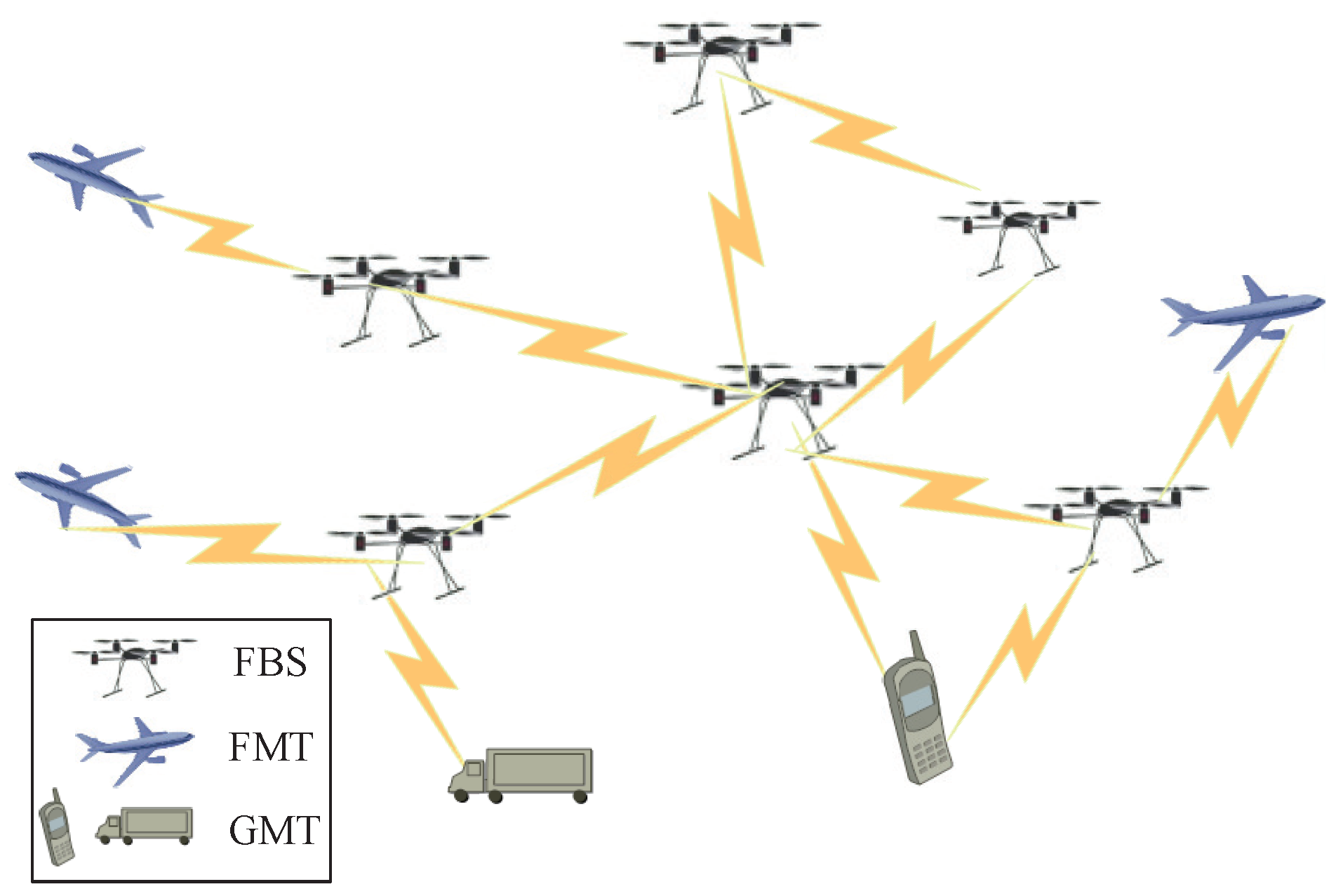
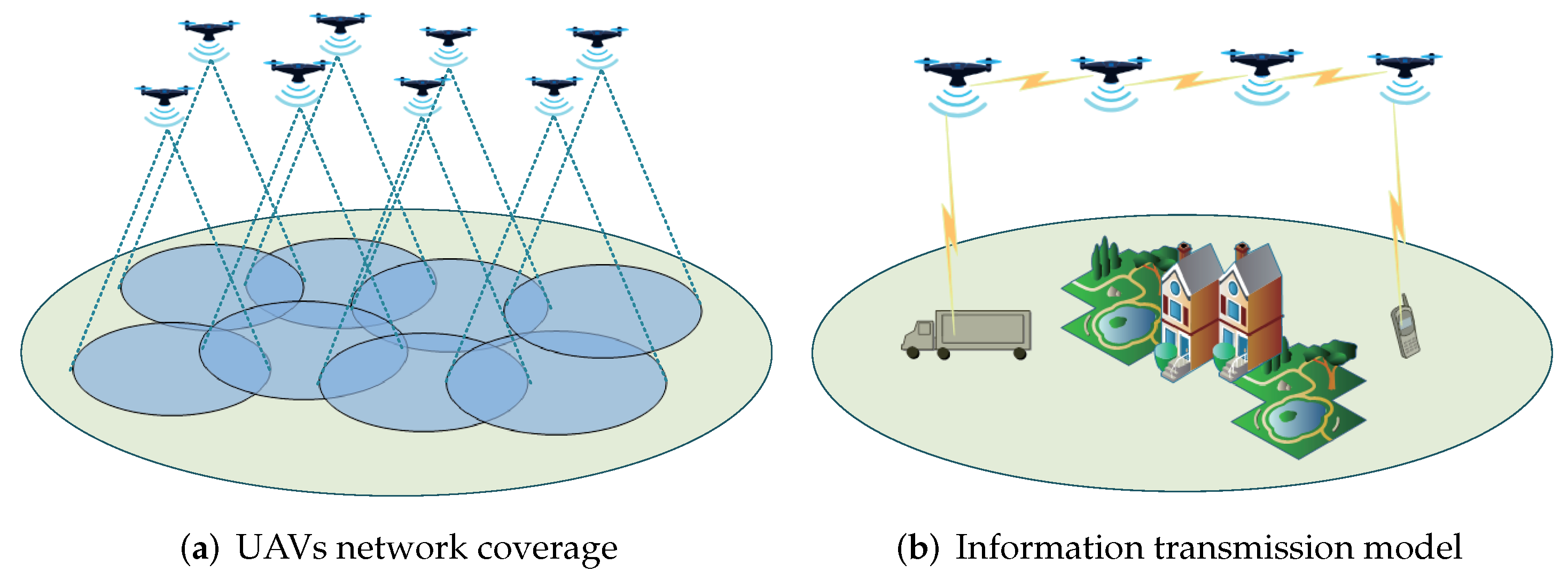
3.2. FlyMesh System Model

In this paper, the multi-hop FlyMesh was established to provide communication services for flight mobile terminals and ground mobile terminals, as shown in in Figure 1. The multi-hop FlyMesh system is composed of a flight base station (FBS), a flight mobile terminal (FMT), and a ground mobile terminal (GMT), which forms a complex network topology. Due to the rapid movement of drones, the topology structure will randomly change.
The information randomly selected a link for data transmission. To facilitate the analysis, we assumed the information transmission at a certain instant, that is, the information was fixed on a particular link for communication. The nodes outside the link were all interference nodes. Simultaneously, UAVs were equipped with directional antennas to reduce the effect of signal interference [29], as shown in Figure 2. The transmission gain g t and the receive gain g r can be described separately as:
g t = 1 + γ cos θ ,
g r = 1 + γ cos φ ,
where θ represents the transmission beam width and φ is the receiving beam width. γ is the degree of influence of beam width on antenna gain. Then, the gain of information transmission between the two nodes can be expressed as:
G = δ g t g r ,
where δ 0 , 1 indicates the degree of alignment of the directional antenna. δ 0 means that the beams are parallel and no information can be sent between nodes, as shown in Figure 2c. δ 1 indicates that the beam is aligned, as shown in Figure 2a. Figure 2b indicates that δ belongs to (0, 1)and its value adjusts with the degree of beam alignment.

4. Performance Probability Analysis

In this paper, we considered the network performance of a multi-hop FlyMesh under β -GPP distribution. We used a more reliable decode-and-forward (DF) protocol. Based on this, the connection probability and ergodic capacity of multi-hop relay were obtained based on the Laplace transform of the interference, and the coverage probability was further derived. In this way, we hoped to describe the network performance of the multi-hop FlyMesh in detail.

4.1. Connection Probability

As shown in Figure 3, information was transmitted from the source node S to the end node D through the relay node R i ( i = 1 , 2 , , N ) . UAVs outside the transmission link were regarded as interference nodes. So, the signal-to-interference-to-noise ratio (SINR) between each hop can be expressed as:
Υ i = P i h i d i α G i r 1 I + T 0 ,
where I = j Φ , i P I d j α h j G j is the total interference received by the relay node, Φ represents the UAVs node in space. The channel gains h j and h i have an exponential distribution with a mean of one. P i and P I indicate the transmission power and interference source power at relay node R i , respectively. r 1 is the interference impact factor. d i is the distance from R i to R i + 1 , and α is the path attenuation factor, which depends on the environment. T 0 is the average background noise power. G i / j can be obtained by (8).
In a multi-hop node information transmission, SINR exists between each hop node. When operating under the DF protocol, according to (9), the end-to-end SINR is expressed as:
Υ D F = min ( Υ 1 , Υ 2 , · · · , Υ N ) .
Then, the connection probability can be expressed as:
P c o n = P ( Υ D F > Q ) .
Since Υ i is independent, from (10) and (11), we can obtain the connection probability P c o n as:
P c o n = F Υ D F ( Q ) = i = 1 N ( 1 F Υ i ( Q ) ) .
Here, F X = P ( X < x ) = 1 exp ( a x ) is an exponential random variable cumulative density function with parameter X. The cumulative density function can be written as:
F Υ i ( Q ) = P h i > Q ( r 1 I + T 0 ) G i P i d i α = E Υ i 1 exp Q ( r 1 I + T 0 ) Θ h G i P i d i α = exp A Υ T 0 L I ( A Υ ) ,
where h i and I are independent, A Υ = Q Θ h G i P i d i α . L I ( X ) is the Laplace transform of a random variable x . Combined with (12), the Laplace transform L I ( A Υ D F ) can be obtained as follows:
L I ( A Υ D F ) = E exp x Φ A Υ P t G j h i ( | x | + ϵ ) β = E x Φ E exp ( A Υ P t G j h i ( | x | + ϵ ) β ) = E x Φ 1 + Θ g A Υ P t G j ( | x | + ϵ ) β 1 = E exp x Φ ln 1 + Θ g A Υ P t G j ( | x | + ϵ ) β .
According to (3), there is
L I ( A Υ ) = D e t I + β K i 1 β ,
and the core matrix K i can be interpreted as:
K i ( x , y ) = Θ g η Υ P I G j Θ g A Υ P I G j + ( | x | + ϵ ) α K ( x , y ) × Θ g A Υ P I G j Θ g η Υ P I G j + ( | y | + ϵ ) α .
We assume
ð ( x ) = Θ g A Υ P I G j Θ g A Υ P I G j + ( x + ϵ ) α .
Denote ζ n as an eigenvalue of K i . Then, the Fredholm determinant of kernek K i can be expressed as
D e t ( I + β K i ) = n 0 ( 1 + β ζ n ) .
Therefore, (15) can be described as
D e t ( I + β K i ) 1 β = n 0 ( 1 + β ζ n ) 1 β .
For simplicity, we introduced a closed form expression for the Fredholm determinant. According to Mercer’s theorem, the kernel K i ( x , y ) can be written as:
K i ( x , y ) = Σ n 0 ζ n ϕ n ( x ) ϕ n ( y ) ¯ ,
where ζ n and ϕ n ( x ) are the basis of eigenvectors and corresponding eigenvalues of K i ( x , y ) , respectively. For x R 2 and n 0 , we can know that ϕ n is an orthogonal basis and ζ n is eigenvalues. There are R 2 ϕ n ( x ) 2 d x = 1 and R 2 ϕ n ( x ) ϕ n ( x ) ¯ d x = 0 . Define
ζ n = 2 ( π ρ ) n + 1 n ! 0 L ð ( x ) 2 exp ( π ρ x 2 ) x 2 n + 1 d x ϕ n ( x ) = ρ v n n ! ð ( | x | ) π ρ x n exp π ρ 2 | x | 2 .
Therefore, D e t ( I + β K i ) 1 β can be represented as:
D e t ( I + β K i ) 1 β = = n 0 1 + 2 β ( π ρ ) n + 1 n ! 0 L exp ( π ρ x 2 ) x 2 n + 1 ð ( x ) 2 d x .
Thus, the connection probability can be rewritten as
P c o n = i = 1 N exp A Υ T 0 × n 0 1 + 2 β ( π ρ ) n + 1 n ! 0 L exp ( π ρ x 2 ) x 2 n + 1 ð ( x ) 2 d x .
It can be seen that the connection probability is influenced by the number of relay nodes, the repulsive parameter, and the beam width. According to (23), the relevant parameters can be adjusted to maintain a high connection probability, ensure the stability of the information link, and improve the reliability of data transmission.

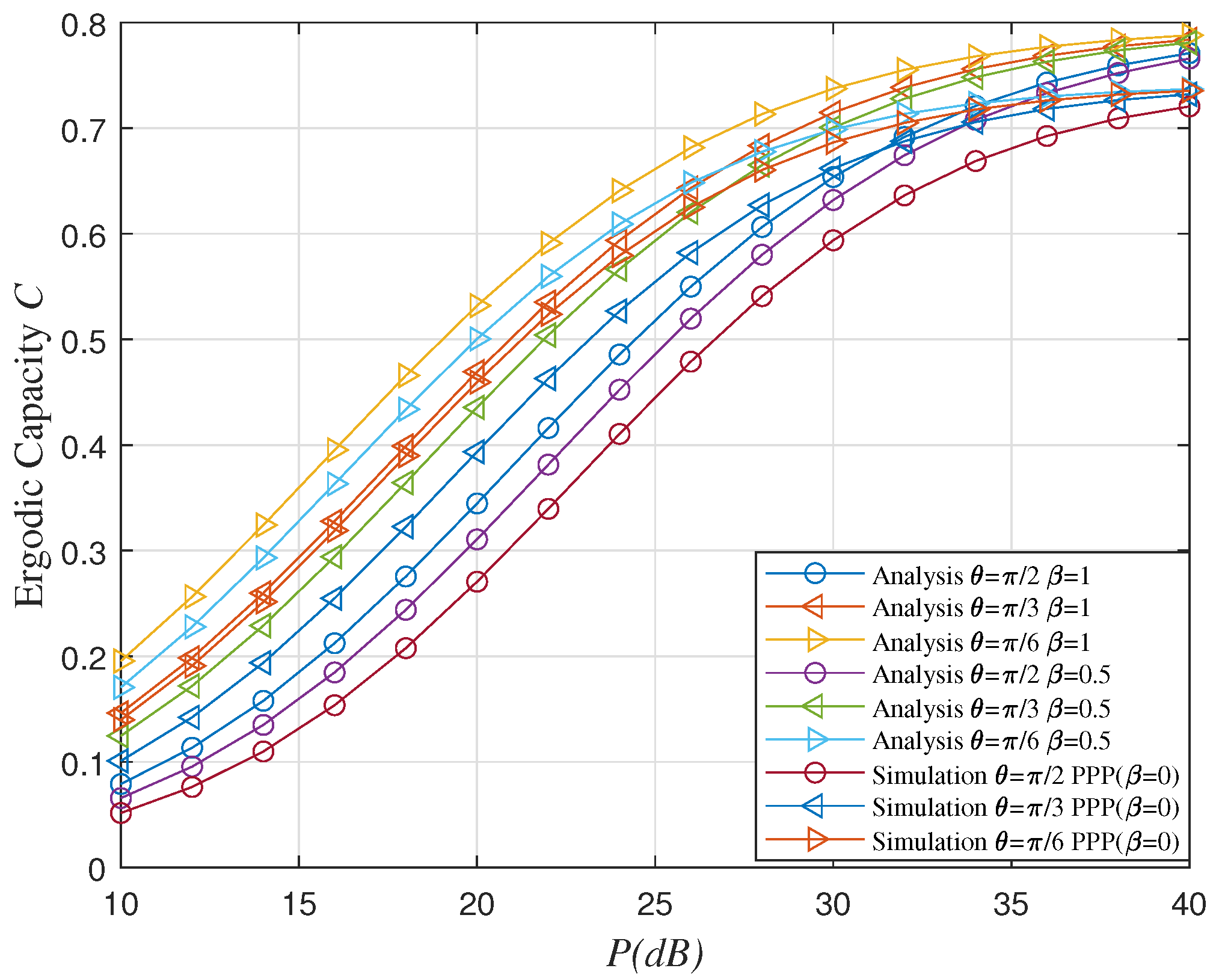
4.2. Ergodic Capacity

According to Shannon, ergodic capacity is a crucial performance metric because it quantifies the maximum achievable transmission rate at which errors can be recovered. In this paper, the DF relay protocol was selected. Specifically, the received signal of each relay station was fully decoded, re-encoded, and then transmitted to the next relay station. The code words transmitted from the source node S were selected from the Gaussian codebook. The minimum capacity of the link determines the capacity of the entire system. On the other hand, according to the minimum cut maximum traffic theorem [30], the overall capacity of the system is less than or equal to the capacity of each link. Then, the ergodic capacity of the ith ( i N ) relay can be expressed as
C i = log ( 1 + Υ i ) .
Therefore, the ergodic capacity of multidirectional multi-hop networks can be given as:
C = min ( C 1 , C 2 , . . . , C N ) .
According to Jensen’s inequality, the upper bound of the ergodic capacity in (25) is
C > 1 N E log ( 1 + Υ i ) = 1 N E min log ( 1 + Υ 1 ) , · · · , log ( 1 + Υ N ) = 1 N E log 1 + min Υ 1 , · · · , Υ N ,
where E ( · ) denotes mathematical expectation. Considering the Taylor series expansion, utilizing partial integration, we can rewrite the traversal capacity as
C = 1 N ln ( 2 ) 0 1 1 + Υ D F ( 1 F Υ i ( Q ) ) d Υ .
Combined with the connection probability, the ergodic capacity can be calculated as
C = 1 N ln ( 2 ) 0 1 1 + Υ D F × i = 1 N exp ( A Υ T 0 ) D e t ( I + β K i ) 1 β d Υ .
The ergodic capacity is derived from the connection probability; thus, we can improve the ergodic capacity while considering the connection probability.

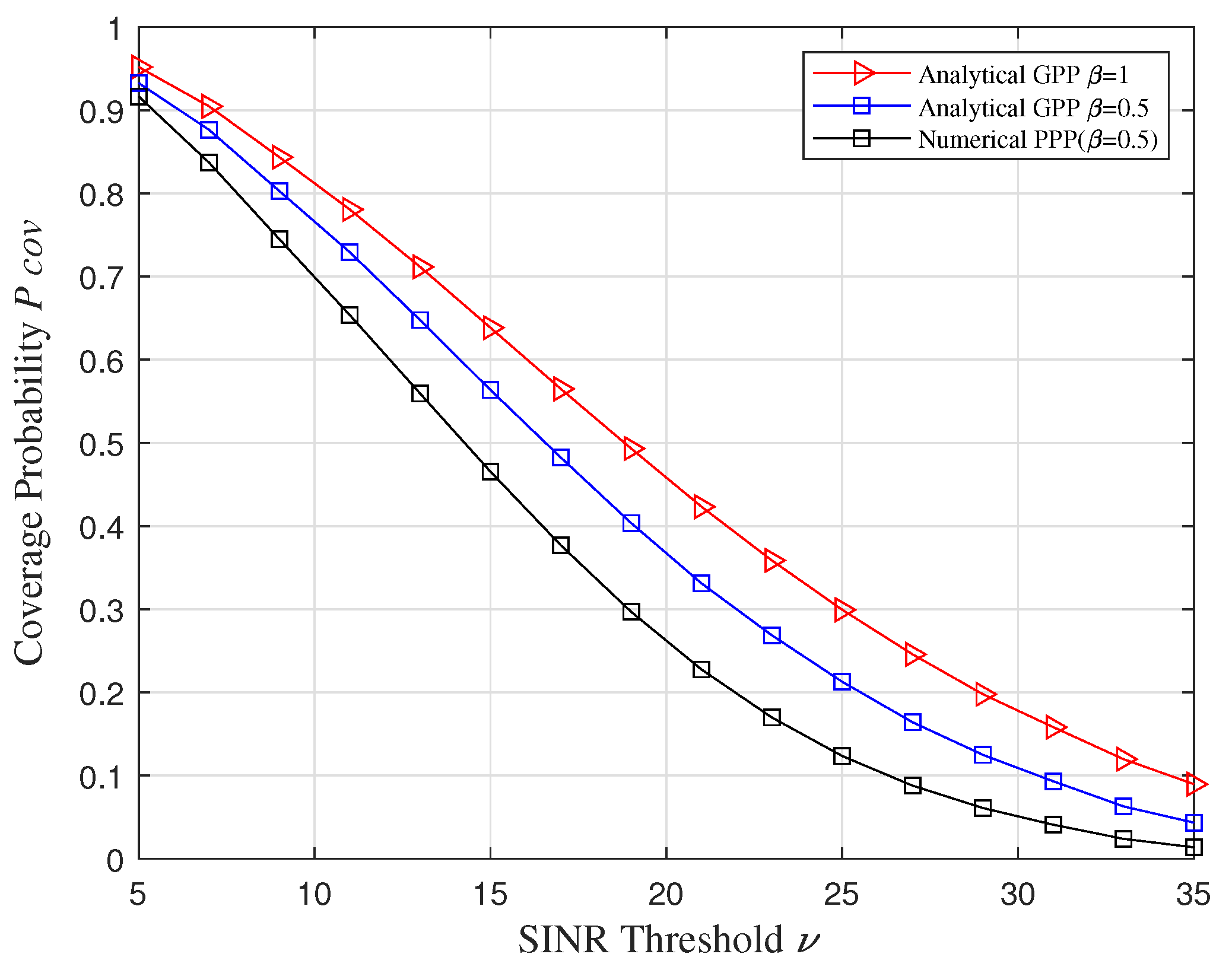
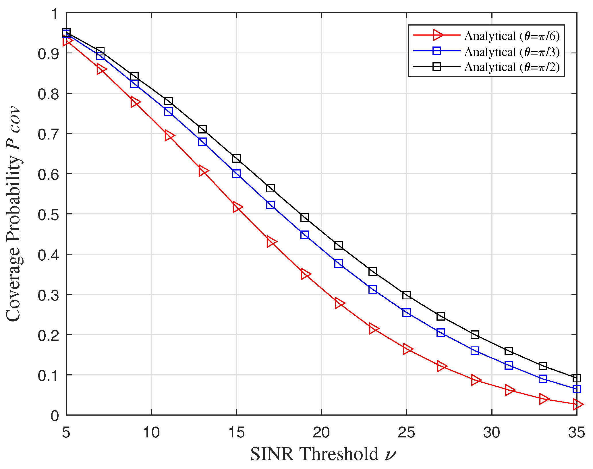
4.3. Coverage Probability

The coverage probability is a measure of the service provided by FlyMesh, as shown in Figure 4. Due to the motion invariance of GPP, we can assume that the coverage probability of a typical user b o ( b o Φ ) is the same at any location. Each typical user is connected to its closest FBS, i.e., the typical user is served by only one closest FBS. Therefore, the coverage probability when SINR is greater than the threshold ν is denoted as:
P c o v = P S I N R > ν , | b o | | b i | = P P t h b o | b o | α G b o r 2 I 2 + σ 2 > ν , | b o | | b i | ,
where P t is the transmit power of the UAVs. h i indicates that the mobile user only experiences Rayleigh fading, which is an exponential random variable with a mean of 1. I = b k Φ \ b o P t h b k | b k | α G b k is the total interference received at the typical user, and r 2 is the interference impact factor. σ 0 denotes the background noise. | · | is the Euclidean distance from the FBS to the user. We usually assume that the path loss exponent α > 2 . G b o / b k can be obtained by (8). Therefore, the coverage probability can be further expressed as:
P c o v = b o = 0 P S I N R > ν b o , | b o | | b i | = | b o | = 0 P h b o > ν r 2 I 2 + σ 2 P t | b o | α G b o , | b o | | b i | f ( b o ) d b o = | b o | = 0 E exp ν σ 2 P t | b o | α G b o exp ν r 2 I 2 P t | b o | α G b o f ( b o ) d b o = | b o | = 0 exp ν σ 2 P t | b o | α G b o L I 2 ( s ) , | b o | | b i | f ( b o ) d b o ,
where s = ν r 2 P t | b o | α G b o , f ( b o ) can be simplified for β -GPP after applying a diagonal approximation as f ( b o ) = 2 c b o e c b o 2 . Therefore, (30) can be written as:
P c o v = | b o | = 0 exp ν σ 2 P t | b o | α G b o L I 2 ( s ) 2 c b o e c b o 2 d b o .
The authors of [31] gave the following expression for the Laplace transform of the interference of a general motion-invariant DPP under the recent FBS correlation scheme, i.e.,
L I 2 ( s ) = E b o [ e s I ] = 0 ( 1 ) n n ! ( R 2 ) n det [ K b o ( b i , b j ) ] 0 ( 1 ) n n ! B ( o , b o ) n det [ K b o ( b i , b j ) ] · · · i = 1 n 1 | b i | | b o | 1 + G b o ν P t | b i | α d b 1 · · · d b n d b 1 · · · d b n .
We used the approximation for the determinant of kernel matrix K b o ( b i , b j )
det [ K b o ( b i , b j ) ] 1 i , j n i = 1 n K b o ( b i , b i ) ,
and we know n = 0 x n n ! = e x . Combined (4) and (5), the (32) can be rewritten as:
E b o ! [ e s I ] = exp ( c π B ( o , b o ) c ( ν G b o P t | b | α ν G b o P t | b | α + 1 + e c β | b b o | 2 ν G b o P t | b | α + 1 e c β | b b o | 2 ) d b ) .
For ease of expression, we split (34) by drawing on Reference [32]; it can be written as:
E b o [ e s I ] = exp c π Θ 1 + Θ 2 + Θ 3 .
Here, we transform the Cartesian coordinate into a polar coordinate system and let | b | = r , Θ 1 can be written as:
Θ 1 = 0 2 π r o ν G b o P t r α ν G b o P t r α + 1 r d r d θ ,
where r denotes the distance to the origin of the polar coordinate system and θ is the polar angle. Replacing r ν 1 α 2 with u, we can get
Θ 1 = π ν 2 α r o ν 1 α 2 G b o P t G b o P t + u α 2 d u .
Equation Θ 2 can be expressed in polar coordinate system as:
Θ 2 = 2 π r o e c β ( r r o ) 2 ν P t r α + 1 r d r .
According to the same method, Θ 3 can be represented as:
Θ 3 = 0 2 π 0 e c β u 2 u d u d θ 2 0 π / 2 0 2 r o c o s ( θ ) e c β u 2 u d u d θ .
For the first part replacing u 2 with y and the second part replacing u 2 with x, we can obtain
Θ 3 = π β c β π 2 c β c 0 4 r o c β 4 r o x d x .
Bringing (37), (38) and (40) into (34), we are able to obtain the expression for the interference Laplace transform under β -GPP as:
L I 2 ( s ) = exp c ν 2 α r o ν 1 α 2 G b o P t G b o P t + u α 2 d u 2 π r o e c β ( r r o ) 2 ν G b o P t r α + 1 r d r + π β c β π 2 c β c 0 4 r o c β 4 r o x d x . .
Combining (41) and (31), P c o v is expressed as:
P c o v = | b o | = 0 exp ν σ 2 P t | b o | α G b o exp c ν 2 α r o ν 1 α 2 P t P t + u α 2 d u + 2 π r o e c β ( r r o ) 2 ν P t r α + 1 r d r + π β c β π 2 c β c 0 4 r o c β 4 r o x d x 2 c b o e c b o 2 d b o .
Coverage probability is the ability of a network to provide a service. The expression shows the effect of the repulsive parameter β and beam width θ on the coverage probability. We can adjust the parameters according to the expression to ensure the ability of the UAVs network to provide services.

5. Numerical Results

This section uses Monte-Carlo methods to verify the correctness of the theoretical analysis. For better validation, some parameters are assumed in Table 1. In order to facilitate the calculation and analysis, the beam width θ = π / 3 is taken according to the adopted mathematical model of antenna gain. We also note that the results of β -GPP corresponding to the actual base station locations have been provided in [20], where the authors showed the accuracy of β -GPP for cellular network modeling by adjusting the parameter β instead of using the analytical results of the derived coverage probabilities. We drew on the same approach β -GPP for the coverage probability curve, based on the fact that the distribution of the squared modes (distances) of the points in β -GPP follows the gamma distribution ([27], Proposition 1).

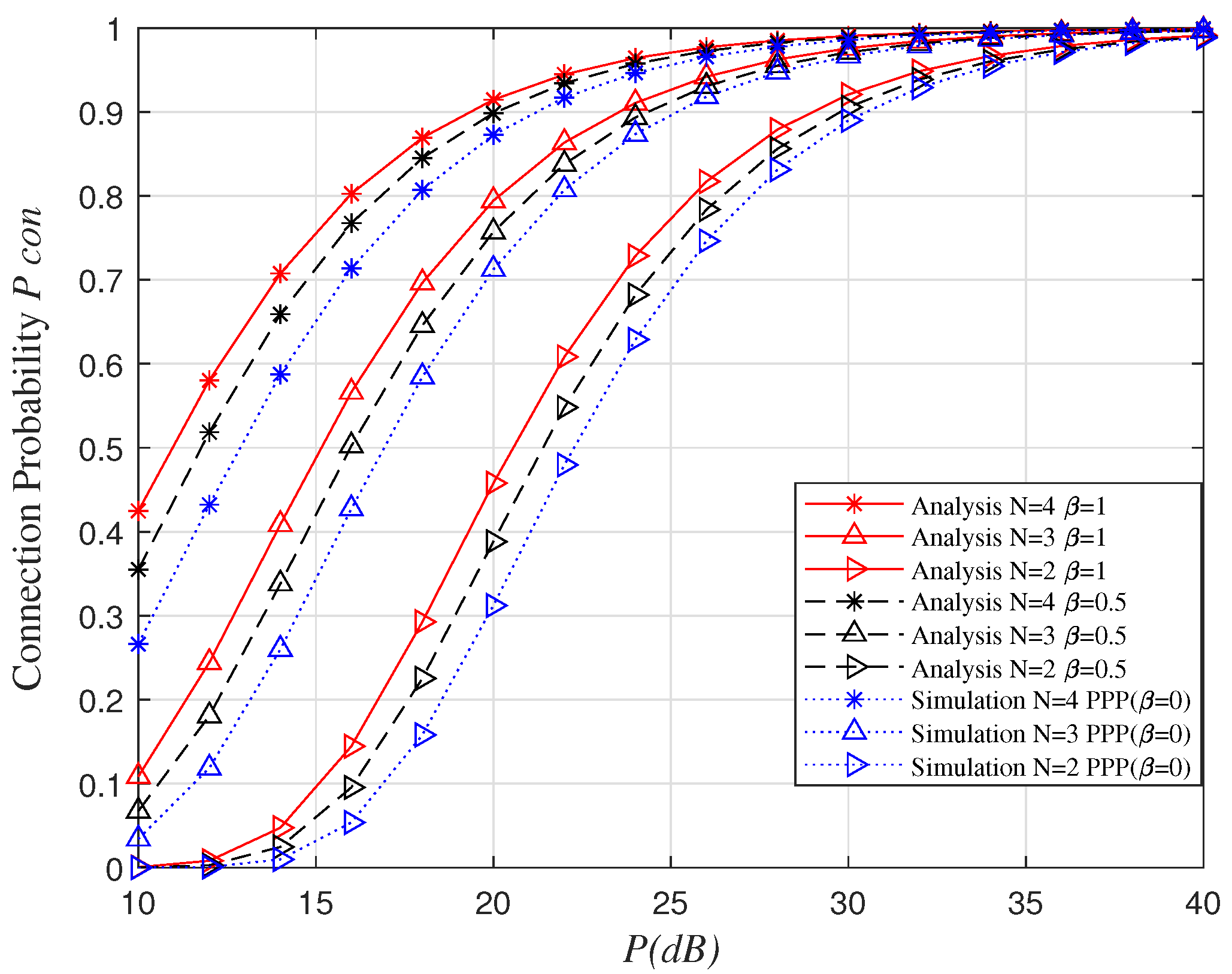
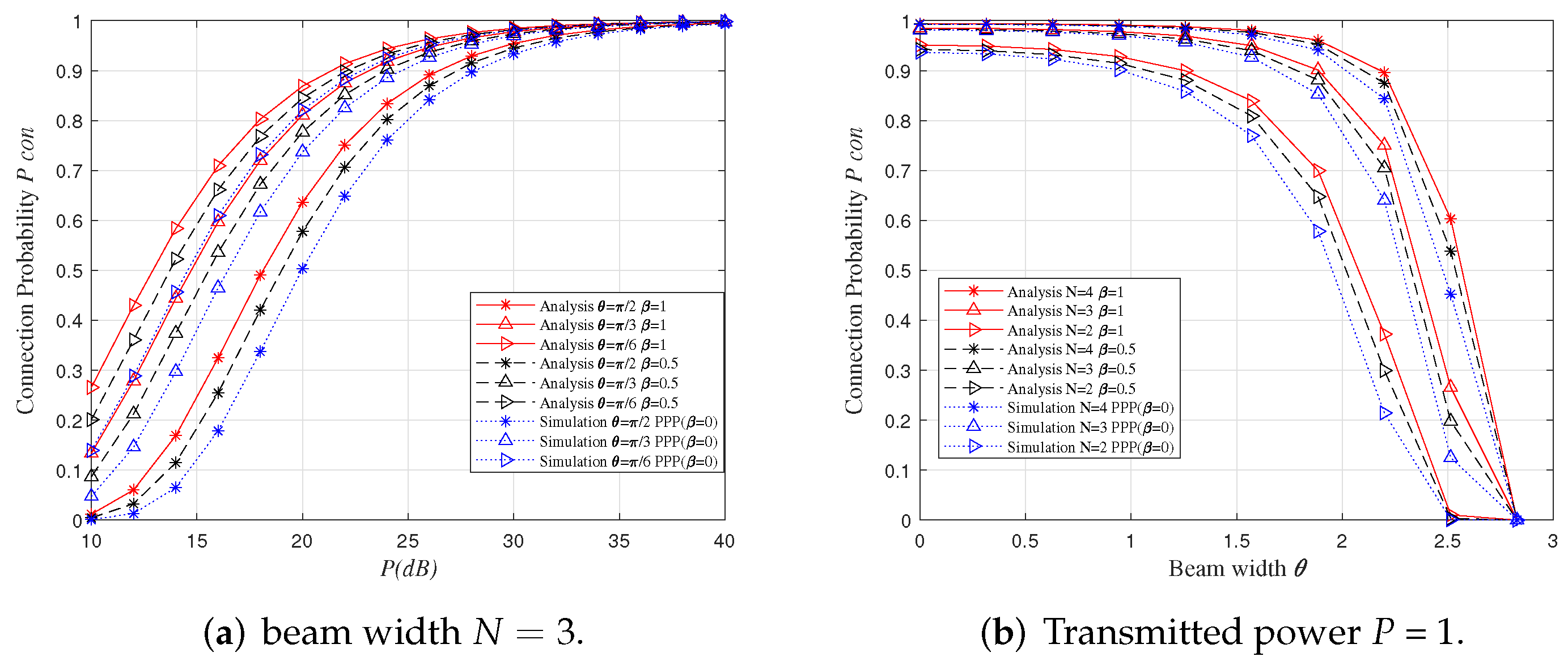
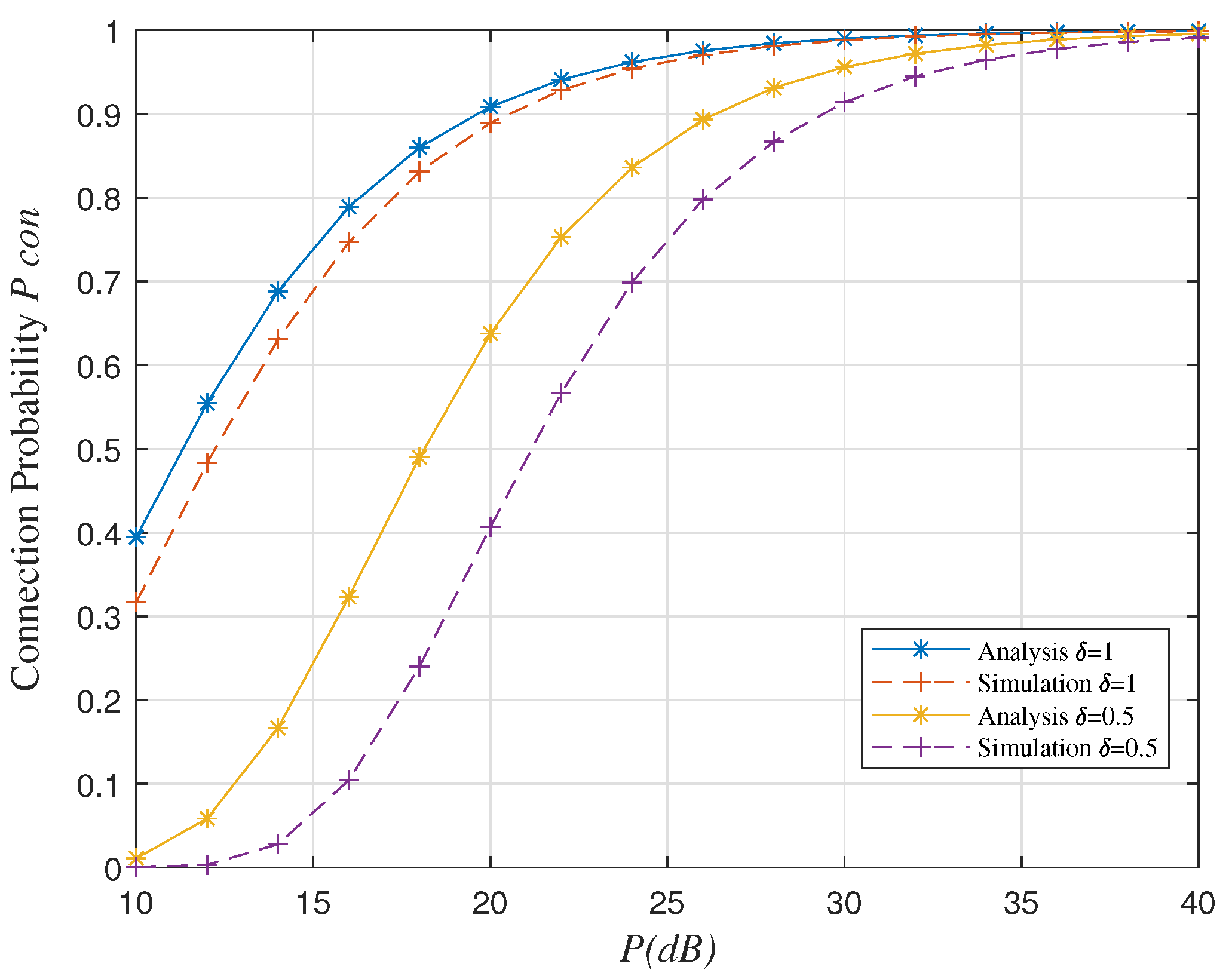
5.1. Connection Probability Verification

Figure 5 shows the relationship between connection probability and the increasing power. The results show that the connection probability increases gradually as the power increases. Additionally, under the same conditions, we can see that the connection probability under the β -GPP model is superior to the PPP model. The more uniform the distribution of the nodes, the higher the connection probability of the network, which indicates that the regular distribution of the nodes reduces the interference between nodes. At the exact β , the connection probability can be increased by increasing the number of hops of relay nodes.
Figure 6a shows the influence of beam width on connection probability under different power. The spatial self-interference is reduced due to the directional antenna, which improves the stability of the connection between the nodes. The connection probability increases as the beam width decreases. It also shows that the connection probability of nodes with a particular regular distribution is better than that of the nodes that are randomly distributed. When the power increases to a certain level, the advantage of antenna gain can be ignored but, at this point, a large amount of energy consumption will increase. Figure 6b shows the relationship between the connection probability and the beam width for the same power. As the beam width increases, the connection probability decreases. However, when the beam width exceeds π , the connection probability decreases significantly, which is due to a sudden increase in signal interference between nodes. Again, it shows that the number of hops of the relay nodes improves the connection probability. Additionally, all the results demonstrate that the distribution rules of the nodes are beneficial for reducing signal interference and improving the connection probability.
Figure 7 illustrates the effect of the degree of beam alignment on the connection probability. The connection probability is highest when the beams are perfectly aligned. The perfect alignment of the beam reduces the signal loss and the information capacity carried can be completely absorbed by the target node, thus improving the information transmission efficiency; otherwise, the energy carried by the beam will be wasted with the directional offset.

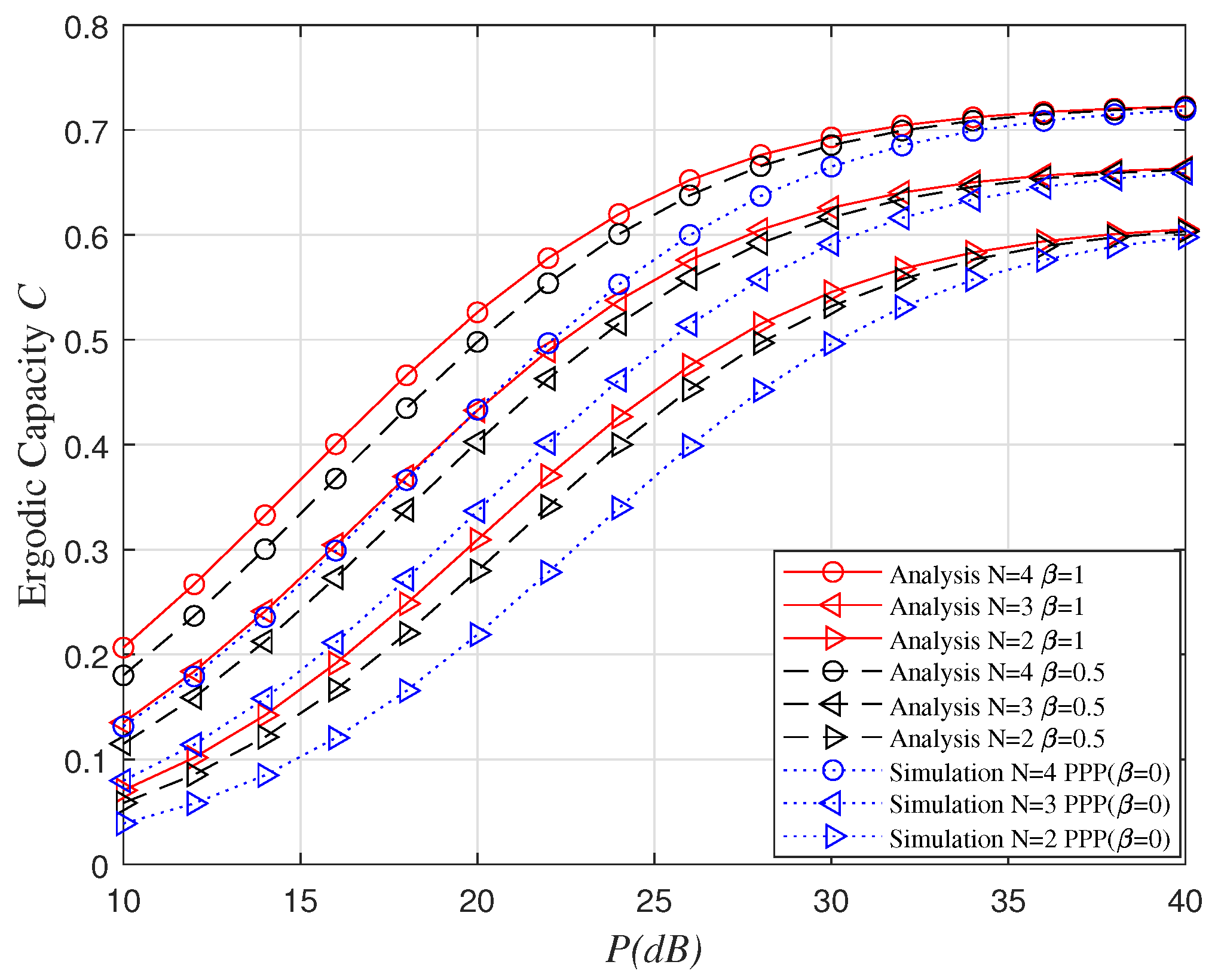
5.2. Ergodic Capacity Verification

Figure 8 shows the relationship between ergodic capacity and power, where the ergodic capacity increases as the power increases. We can see that the more hops of relay nodes, the higher the ergodic capacity. This phenomenon is directly related to the connection probability. At the same time, the ergodic capacity of nodes under specific regular distribution is more significant than that under the PPP model, which is still due to the self-interference reduction.
The effect of different beam widths on the ergodic capacity is shown in Figure 9. The directionality of the antenna increases the antenna gain and also increases the traversal capacity. The directionality of the antenna concentrates the energy and improves the efficiency of information transmission. Interference is also a factor that affects the traversal capacity, and the uniform deployment of nodes is beneficial for capacity improvement.

5.3. Coverage Probability Verification

Figure 10 depicts the relationship between the threshold and the coverage probability for different β . As β increases, the negative correlation between points increases, so the distribution of nodes becomes more regular and most of the disturbances are restricted to areas closer to a point. Therefore, the regularity leads them to cover a wider area. Figure 11 describes the coverage probability for different beam widths. The directionality of the beam helps to increase the connection probability but decreases the coverage probability, which is due to the fact that assigning a shape to the beam reduces the width of the beam. Therefore, we need to consider that the beam width can be adjusted to keep the performance of the whole network balanced.

6. Conclusions

In this paper, we analyzed a multi-hop FlyMesh based on a β -GPP distribution. The location distribution of UAVs followed a β -GPP model, which was a scalable UAV network. We simulated the the deployment of FlyMesh in different environments by adjusting the repulsive parameter β , which was the degree of exclusion between control points. Neglecting the small-scale fading between interfering links, we derived an approximate expression for the connection probability utilizing stochastic geometry and further obtained the ergodic capacity. Finally, we obtained an approximate expression of the coverage probability using an approximation of the diagonal core matrix to analyze the ability of FlyMesh to provide services. The results of the performance analysis provide theoretical guidance for deploying multi-hop FlyMesh in different environments. For example, in a densely populated urban environment, UAVs can be deployed evenly. At this time, the rejection factor β 1 . Engineers can set the beam width to θ and the number of relay hops to N according to the rejection factor to improve the overall network performance.

Author Contributions

Conceptualization, S.Q., R.X., L.P. and X.W. (Xingchen Wei); methodology, S.Q., R.X.; software, X.W. (Xingchen Wei) and D.J.; validation, S.Q., X.W. (Xingchen Wei) and D.J.; writing—original draft preparation, S.Q.; writing—review and editing, S.Q., L.P., X.W. (Xingchen Wei); supervision, R.X., L.P.; funding acquisition, R.X., L.P. All authors have read and agreed to the published version of the manuscript.

Funding

This work is supported by the National Natural Science Foundation of China (No. 61671471).

Institutional Review Board Statement

Not applicable.

Informed Consent Statement

Not applicable.

Data Availability Statement

No new data were created or analyzed in this study. Data sharing is not applicable to this article.

Conflicts of Interest

The authors declare no conflict of interest.

Abbreviations

The following abbreviations are used in this manuscript:
UAVsUnmanned aerial vehicles
IoTInternet of Things
FlyMeshflying mesh network
β -GPP β -Ginibre point process
PPPPoisson point process
IPPPinhomogeneous Poisson point process
DPPdeterministic point process
FBSflying base station
FMTflying mobile terminal
GMTground mobile terminal
DFdecode-and-forward
SINRsignal-to-interference-plus-noise ratio

References

  1. Huang, H.; Savkin, A.V. Deployment of heterogeneous UAV base stations for optimal quality of coverage. IEEE Internet Things J. 2022, 9, 16429–16437. [Google Scholar] [CrossRef]
  2. Ding, R.; Chen, J.; Wu, W.; Liu, J.; Gao, F.; Shen, X. Packet routing in dynamic multi-hop UAV relay network: A multi-agent learning approach. IEEE Trans. Veh. Technol. 2022, 71, 10059–10072. [Google Scholar] [CrossRef]
  3. Chen, Y.; Zhao, N.; Ding, Z.; Alouini, M.-S. Multiple UAVs as Relays: Multi-Hop Single Link Versus Multiple Dual-Hop Links. IEEE Trans. Wirel. Commun. 2018, 17, 6348–6359. [Google Scholar] [CrossRef]
  4. Izydorczyk, T.; Berardinelli, G.; Mogensen, P.; Ginard, M.M.; Wigard, J.; Kovács, I.Z. Achieving High UAV Uplink Throughput by Using Beamforming on Board. IEEE Access 2020, 8, 82528–82538. [Google Scholar] [CrossRef]
  5. Bekmezci, I.; Sahingoz, O.K.; Temel, Ş. Flying ad-hoc networks (FANETs): A survey. Ad Hoc Netw. 2013, 11, 1254–1270. [Google Scholar] [CrossRef]
  6. Haenggi, M. Stochastic Geometry for Wireless Networks; Cambridge University Press: Cambridge, UK, 2012. [Google Scholar]
  7. Lahmeri, M.-A.; Kishk, M.A.; Alouini, M.-S. Laser-Powered UAVs for Wireless Communication Coverage: A Large-Scale Deployment Strategy. IEEE Trans. Wirel. Commun. 2023, 22, 518–533. [Google Scholar] [CrossRef]
  8. Goldman, A. The Palm measure and the Voronoi tessellation for the Ginibre process. Ann. Appl. Probab. 2010, 20, 90–128. [Google Scholar] [CrossRef]
  9. Matracia, M.; Kishk, M.A.; Alouini, M.-S. Coverage analysis for UAV-assisted cellular networks in rural areas. IEEE Open J. Veh. Technol. 2021, 2, 194–206. [Google Scholar] [CrossRef]
  10. Mozaffari, M.; Saad, W.; Bennis, M.; Debbah, M. Unmanned aerial vehicle with underlaid device-to-device communications: Performance and tradeoffs. IEEE Trans. Wirel. Commun. 2016, 15, 3949–3963. [Google Scholar] [CrossRef]
  11. Choi, C.-S.; Baccelli, F.; Veciana, G.D. Modeling and analysis of data harvesting architecture based on unmanned aerial vehicles. IEEE Trans. Wirel. Commun. 2019, 19, 1825–1838. [Google Scholar] [CrossRef]
  12. Xiong, Z.; Zhang, Y.; Lim, W.Y.B.; Kang, J.; Niyato, D.; Leung, C.; Miao, C. UAV-assisted wireless energy and data transfer with deep reinforcement learning. IEEE Trans. Cogn. Commun. Netw. 2021, 7, 85–99. [Google Scholar] [CrossRef]
  13. Ng, J.S.; Ng, W.C.; Lim, W.Y.B.; Xiong, Z.; Niyato, D.; Leung, C.; Miao, C. UAV-assisted Wireless Power Charging for Efficient Hybrid Coded Edge Computing Network. In Proceedings of the ICC 2022-IEEE International Conference on Communications, Seoul, Republic of Korea, 16–20 May 2022; pp. 4037–4042. [Google Scholar]
  14. Wei, X.; Cai, L.; Wei, N.; Zou, P.; Zhang, J.; Subramaniam, S. Joint UAV Trajectory Planning, DAG Task Scheduling, and Service Function Deployment based on DRL in UAV-empowered Edge Computing. IEEE Internet Things J. 2023. [Google Scholar] [CrossRef]
  15. Armeniakos, C.K.; Kanatas, A.G. Performance Comparison of Wireless Aerial 3D Cellular Network Models. IEEE Commun. Lett. 2022, 26, 1779–1783. [Google Scholar] [CrossRef]
  16. Guo, X.; Zhang, C.; Yu, F.; Chen, H. Coverage analysis for UAVassisted mmwave cellular networks using Poisson hole process. IEEE Trans. Veh. Technol. 2022, 71, 3171–3186. [Google Scholar] [CrossRef]
  17. Lavancier, F.; Møller, J.; Rubak, E. Determinantal point process models and statistical inference. J. Roy. Stat. Soc. B (Stat. Methodol.) 2015, 77, 853–877. [Google Scholar] [CrossRef]
  18. Kong, H.B.; Flint, I.; Wang, P.; Niyato, D.; Privault, N. Exact performance analysis of ambient RF energy harvesting wireless sensor networks with Ginibre point process. IEEE J. Sel. Areas Commun. 2016, 34, 3769–3784. [Google Scholar] [CrossRef]
  19. Zhang, C.; Yu, F.; Wang, Z.; Lyu, G. Performance Analysis of Clustered Wireless-Powered Ad Hoc Networks via β-Ginibre Point Processes. IEEE Trans. Wirel. Commun. 2021, 20, 7475–7489. [Google Scholar] [CrossRef]
  20. Deng, N.; Zhou, W.; Haenggi, M. The Ginibre point process as a model for wireless networks with repulsion. IEEE Trans. Wirel. Commun. 2015, 14, 107–121. [Google Scholar] [CrossRef]
  21. Kong, H.-B.; Wang, P.; Niyato, D. Performance Analysis of Multihop Relaying Systems in an α-Ginibre Field of Interferers. IEEE Trans. Veh. Technol. 2017, 66, 7573–7577. [Google Scholar] [CrossRef]
  22. Kong, H.-B.; Wang, P.; Niyato, D. Performance analysis of wireless sensor networks with ginibre point process modeling. In Proceedings of the 2017 IEEE International Conference on Communications (ICC), Paris, France, 21–25 May 2017; pp. 1–6. [Google Scholar]
  23. Guo, J.; Walk, P.; Jafarkhani, H. Optimal Deployments of UAVs With Directional Antennas for a Power-Efficient Coverage. IEEE Trans. Commun. 2020, 68, 5159–5174. [Google Scholar] [CrossRef]
  24. Tyrovolas, D.; Tegos, S.A.; Diamantoulakis, P.D.; Karagiannidis, G.K. Synergetic UAV-RIS Communication With Highly Directional Transmission. IEEE Wirel. Commun. Lett. 2022, 11, 583–587. [Google Scholar] [CrossRef]
  25. Peng, J.; Tang, W.; Zhang, H. Directional Antennas Modeling and Coverage Analysis of UAV-Assisted Networks. IEEE Wirel. Commun. Lett. 2022, 11, 2175–2179. [Google Scholar] [CrossRef]
  26. Chen, S.; Sun, S.; Xu, G.; Su, X.; Cai, Y. Beam-Space Multiplexing: Practice, Theory, and Trends, From 4G TD-LTE, 5G, to 6G and Beyond. IEEE Trans. Commun. 2020, 27, 162–172. [Google Scholar]
  27. Shirai, T.; Takahashi, Y. Random point fields associated with certain Fredholm determinants I: Fermion, poisson and boson point processes. J. Funct. Anal. 2003, 205, 414–463. [Google Scholar] [CrossRef]
  28. Miyoshi, N.; Shirai, T. A cellular network model with Ginibre configured base stations. Adv. Appl. Probab. 2014, 46, 832–845. [Google Scholar] [CrossRef]
  29. Georgiou, O.; Wang, S.; Bocus, M.Z.; Dettmann, C.P.; Coon, J.P. Directional antennas improve the link-connectivity of interference limited ad hoc networks. In Proceedings of the 2015 IEEE 26th Annual International Symposium on Personal, Indoor, and Mobile Radio Communications (PIMRC), Hong Kong, China, 30 August–2 September 2015; pp. 1311–1316. [Google Scholar]
  30. Huang, C.; Zhang, R.; Cui, S. Throughput Maximization for the Gaussian Relay Channel with Energy Harvesting Constraints. IEEE J. Sel. Areas Commun. 2013, 31, 1469–1479. [Google Scholar] [CrossRef]
  31. Li, Y.; Baccelli, F.; Dhillon, H.S.; Andrews, J.G. Statistical modelling and probabilistic analysis of cellular networks with determinantal point processes. IEEE Trans. Wirel. Commun. 2015, 63, 3405–3422. [Google Scholar] [CrossRef]
  32. Ali, A.; Vesilo, R. Interference Modelling in Cellular Networks with beta-Ginibre Point Process Deployed Base Stations. In Proceedings of the 2017 IEEE 85th Vehicular Technology Conference (VTC Spring), Sydney, NSW, Australia, 4–7 June 2017; pp. 1–6. [Google Scholar]
Figure 1. FlyMesh model.
Drones 07 00335 g001
Figure 2. Three different alignment modes between beams: a, b, c.
Drones 07 00335 g002
Figure 3. Multi-hop UAVs relay system based on β -GPP.
Drones 07 00335 g003
Figure 4. A multi-hop relay UAVs coverage model based on β -GPP distribution, where the coverage probability of the UAVs network is equal at each location.
Drones 07 00335 g004
Figure 5. Connection probability versus P with different N and node deployment, where sita = pi/3.
Drones 07 00335 g005
Figure 6. The connection probability is influenced by the number of relay nodes N and the repulsive parameter β .
Drones 07 00335 g006
Figure 7. The degree of alignment of the directional antenna to the connection probability.
Drones 07 00335 g007
Figure 8. The ergodic capacity as a function of P for different numbers of relay hops.
Drones 07 00335 g008
Figure 9. The ergodic capacity as a function of P at different beam width.
Drones 07 00335 g009
Figure 10. Comparison of coverage probabilities at different beam widths.
Drones 07 00335 g010
Figure 11. Comparison of coverage probabilities under different repulsion factors.
Drones 07 00335 g011
Table 1. Simulation parameters.
DefinitionParametersValues
End-to-end distanced i = 1 N d i
Interference power coefficientk P I / P
Transmission power coefficient P i P
Effective signal coefficient Θ h , Θ g 1
Threshold valueQ1
Background noise T 0 1
Length coefficientL30
Disclaimer/Publisher’s Note: The statements, opinions and data contained in all publications are solely those of the individual author(s) and contributor(s) and not of MDPI and/or the editor(s). MDPI and/or the editor(s) disclaim responsibility for any injury to people or property resulting from any ideas, methods, instructions or products referred to in the content.

