Distributed Bearing-Only Formation Control for UAV-UWSV Heterogeneous System

Abstract

This paper investigates the bearing-only formation control problem of a heterogeneous multi-vehicle system, which includes unmanned aerial vehicles (UAVs) and unmanned surface vehicles (UWSVs). The interactions among vehicles are described by a particular class of directed and acyclic graphs, namely heterogeneous leader-first follower (HLFF) graphs. Under the HLFF structure, a UAV is selected as the leader, moving with the reference dynamics, while the followers, including both UAVs and UWSVs, are responsible for controlling the position with regard to the neighbors in the formation. To solve the problem, we propose a velocity-estimation-based control scheme, which consists of a distributed observer for estimating the reference velocity of each vehicle and a distributed formation control law for achieving the desired formation based on the estimations and bearing measurements. Moreover, it is shown that the translation and scale of the formation can be uniquely determined by the leader UAV. The theoretical analysis demonstrated the finite-time convergence of the velocity estimation and the asymptotic convergence of the formation tracking. Comparative simulation results are provided to substantiate the effectiveness of the proposed method.

1. Introduction

With excellent autonomy and control ability, unmanned aerial vehicles (UAVs) play an important role in various engineering applications [1,2,3]. Contrary to a single UAV for solo operation, the cooperation of multiple UAVs and their formation control have received increasing attention over the past decades [4,5,6,7,8,9]. However, in the field of maritime emergency search and rescue (MESAR), UAVs with airborne cameras are capable of searching quite a long range for targets, but their further application in MESAR is mainly restricted by limited battery supply and the lack of the perception of the close-quarter maritime environment. Conversely, unmanned water surface vehicles (UWSVs) with sufficient power supply and close-quarter surface detection systems can effectively overcome the power and perception deficiencies of UAVs. Whereas UWSVs have a limited perception of a wide range of surrounding dynamic environments, resulting in adverse effects on navigation safety. By contrast, the cooperation of UAVs and UWSVs can benefit from the advantages of both and improve the efficiency and robustness of MESAR missions. Thus, the coordination control of the UAV-UWSV system is meaningful and should be further studied [10,11].

It should be noted that the UAV-UWSV system is typically heterogeneous, i.e., with non-identical dynamic representations [12], which renders the coordination control methods for homogeneous multiagent systems unavailable. There have been some great works on UAV-UWSV systems. The authors of [13] studied the cooperative path-following problem of UAV-UWSV systems based on dynamic surface control and event-triggered techniques. In [14], a spatial mapping guidance law was developed to provide the reference heading angles for the UAV and UWSV, and an adaptive fuzzy control law was subsequently designed to track the reference path. Authors of [15] proposed a cooperative UAV-UWSV platform and a dynamic positioning algorithm to guarantee that UAVs can land on the UWSV steadily. Note that [13,14,15] particularly focused on a single pair of UAV-UWSV. Ref. [16] addressed the formation control problem of a UAV-UWSV heterogeneous multiagent system and provided sufficient conditions to achieve the consensus. In [17], a distributed formation protocol was proposed such that the leader UAV and follower UWSVs track the desired trajectory and achieve the desired formation simultaneously. Ref. [18] proposed a formation control protocol for a UAV-UWSV heterogeneous system based on leader-following distributed consensus and artificial potential field. Nevertheless, the above-mentioned studies are based on the assumption that "the global positioning is available for UAVs and UWSVs", which heavily relies on external infrastructure and high-accuracy sensors and, therefore, is difficult to set up in a harsh maritime environment. Due to the accessibility of relative bearings by vision-based localization systems and wireless sensor arrays, a bearing-only control protocol is promising to perform the MESAR tasks via onboard sensors.

There have been numerous works on bearing-only formation control. Early studies such as [19,20] focused on the bearing angle between neighbor agents to achieve the target formation, but it is limited to 2D circumstances. On the basis of bearing rigidity [21], the relative bearing vector is now mostly employed to overcome this limitation. In [22], bearing-only formation control laws were designed for single-integrator, double-integrator and nonholonomic vehicles to achieve formation tracking control in cases where the leaders move with constant velocity. In [23], a velocity-estimation-based formation control scheme was proposed, which solved the problem of the time-varying velocity of leaders. Authors in [24] designed a bearing-only control law for networked robots with nonholonomic constraints. Ref. [25] presented a finite-time bearing-only formation control scheme, wherein a finite-time orientation estimator was incorporated to remove the dependence on global coordination frame. It is worth noting that the communication and sensing graphs in [22,23,24,25] are assumed to be bidirectional, i.e., we should keep constant mutual visibility among all inter-agent pairs. This is difficult to satisfy due to the limited field of view. To remove such a constraint, [26] proposed bearing-based control laws under a particular directed graph, namely the leader-first follower (LFF) structure, which can be generated via bearing-based Henneberg construction. The LFF graph has a promising feature in that the translation of the formation is determined by the leader, and the formation scaling motion is determined by the relative distance between the leader and the first follower; thus, the formation’s maneuvers can be flexibly managed. Motivated by this, we have recently studied bearing-based formation control problems for UAVs [27] and UWSVs [28] with LFF structures. However, the methods in [26,27,28] were not bearing-only because the distance between the leader and the first follower should be measured accurately in order to maintain the formation scale.

Another thing worth mentioning is that the above methods concentrated on homogeneous multiagent systems, and, therefore, cannot be applied to a UAV-UWSV heterogeneous system. Ref. [29] studied finite-time bearing-only formation control problem of heterogeneous multi-robot systems with collision avoidance, however, the order of each robot is assumed to be identical. In our mix-order UAV-UWSV system, UAVs can navigate in three-dimensional (3D) space, while the UWSVs maneuver in the two-dimensional (2D) plane. This results in more difficulties, since the UWSVs can measure the 3D relative bearing vectors to the neighboring UAVs but are only allowed to translate in the horizontal plane in order to maintain the desired 3D bearings. In other words, the formation control problem of UAV-UWSV systems is subject to spatial constraints, which makes it more complex and difficult. To the best of the authors’ knowledge, the bearing-only formation control problem for UAV-UWSV heterogeneous multiagent system is hitherto rare.

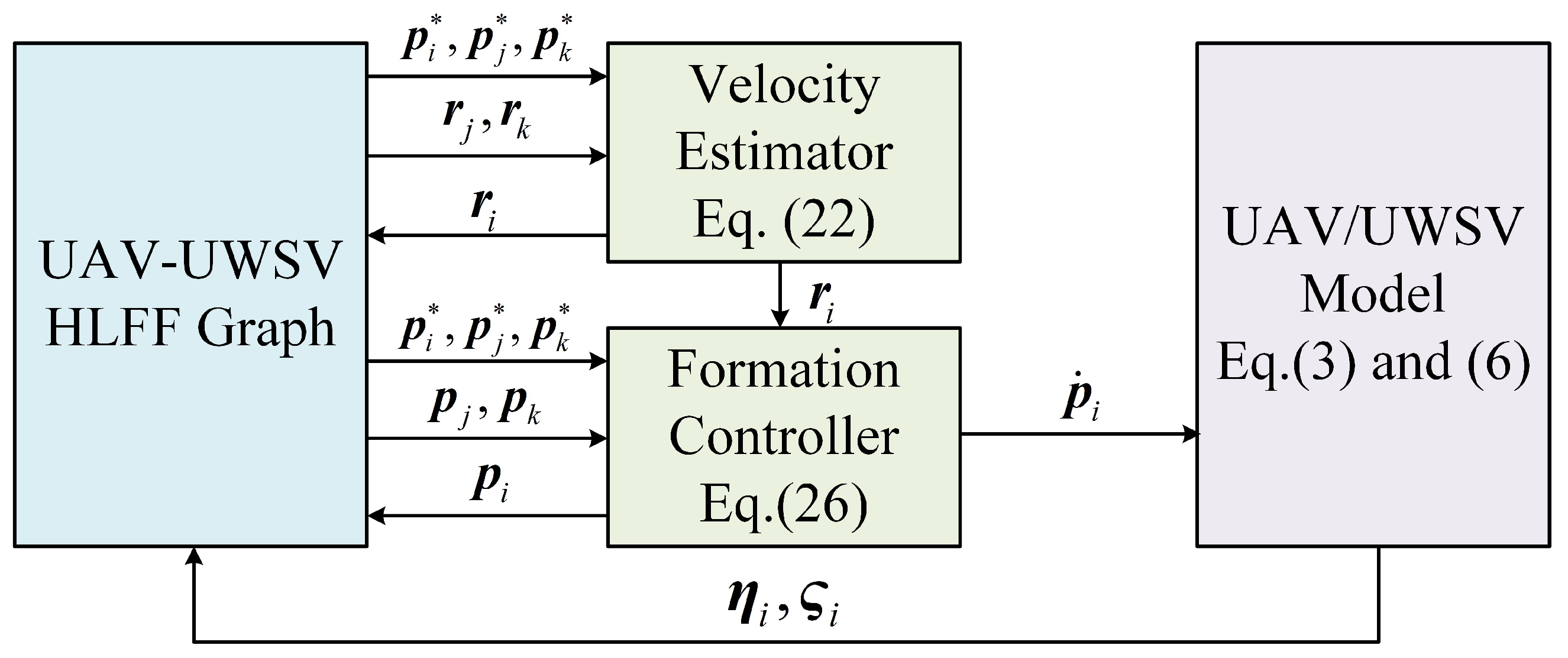
Motivated by the above discussions, we propose a novel bearing-only formation control scheme for a UAV-UWSV heterogeneous multiagent system. We first describe the communication and sensing networks of the system via a directed and acyclic graph called the heterogeneous leader-first follower (HLFF) graph. On this basis, a velocity-estimation-based control scheme is proposed, which consists of a finite-time distributed observer for estimating the reference velocity of each follower and a bearing-only formation control law to achieve the desired formation without global positioning. It is shown that the formation tracking error converges to zero asymptotically. The main contributions of this article are summarized as follows.

• We extend the LFF graph for the homogeneous multiagent systems to the HLFF graph for the heterogeneous system. The HLFF graph is verified to have distinct properties from LFF graphs as a single-leader bearing-only graph since both the translation and scale of the formation can be uniquely determined by the position of the leader other than the position of the leader and its distance between the leader and the first follower. Thus the distance measurements between the leader and the first follower are not required as [26,27,28].
• Compared with the existing control methods for UAV-UWSV systems [13,14,15,16,17,18], which heavily rely on global positioning, our proposed control scheme only requires relative bearing vectors between neighboring vehicles, which can be obtained via onboard sensors such as vision cameras and sensing arrays.
• Different from the bearing-only formation control for a homogeneous system [22,23,24,25] and a heterogeneous system with identical system order [29], our proposed formation protocol can be applied to heterogeneous mixed-order systems, which is more challenging and complex as some agents have spatial constraints.

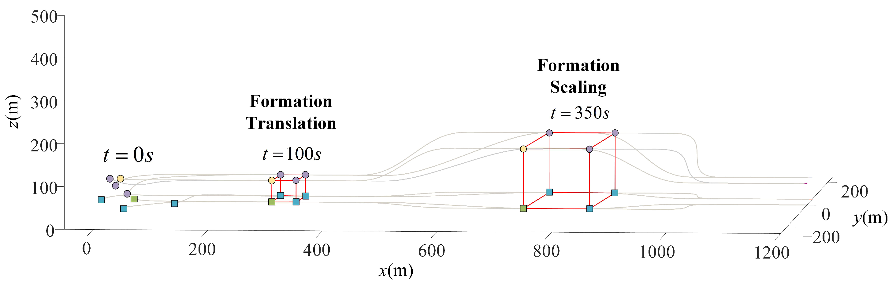
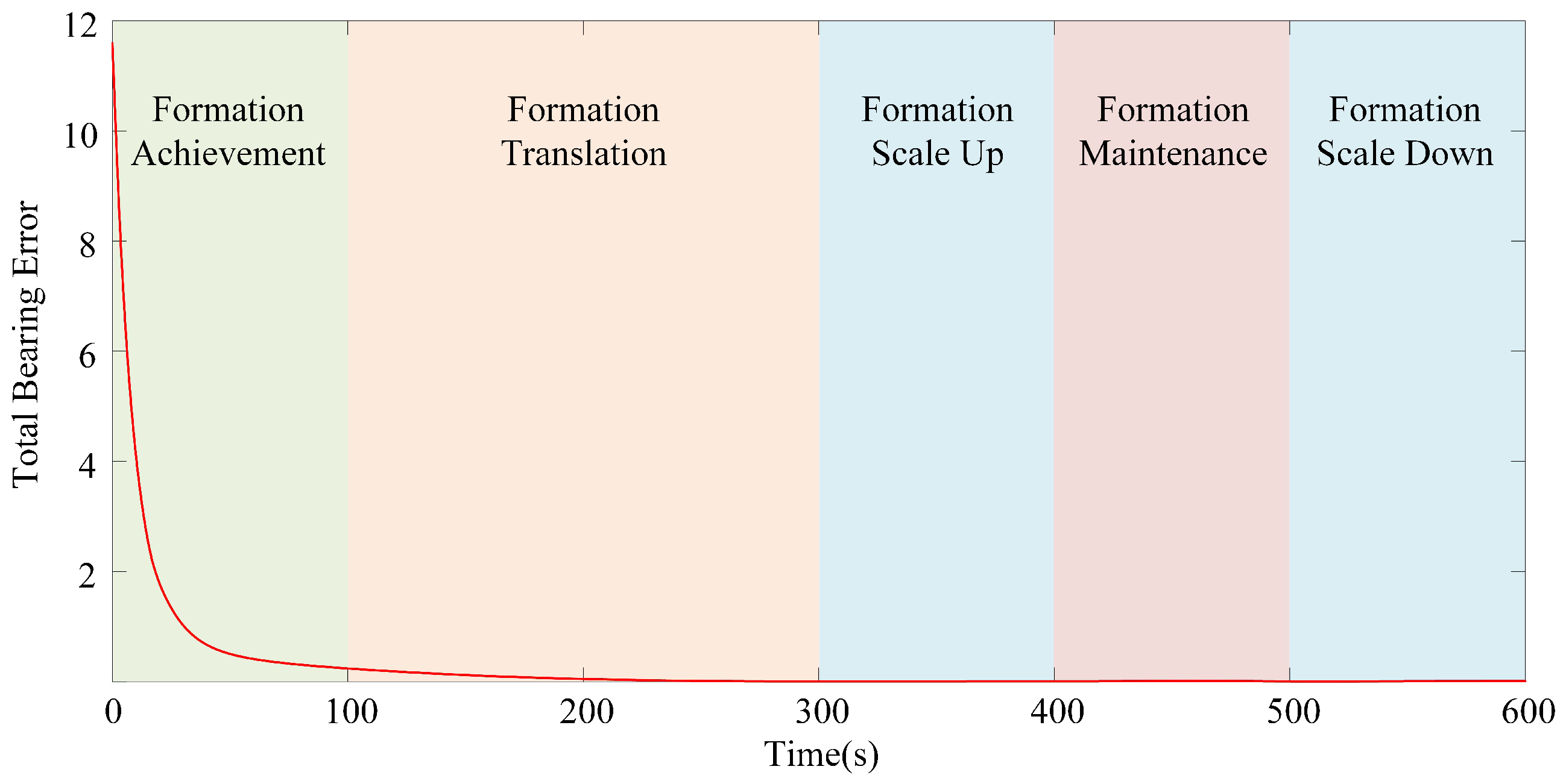
The remainder of this paper is organized as follows: Section 2 presents the preliminaries and formulates the bearing-only formation control problem for a UAV-UWSV heterogeneous system. The proposed unified formation control scheme, including finite-time distributed observer and bearing-only formation control law, is detailed in Section 3. The comparative simulation results are presented in Section 4, after which we conclude the paper.

2. Preliminaries and Problem Formulation

2.1. Model of UAV and UWSV

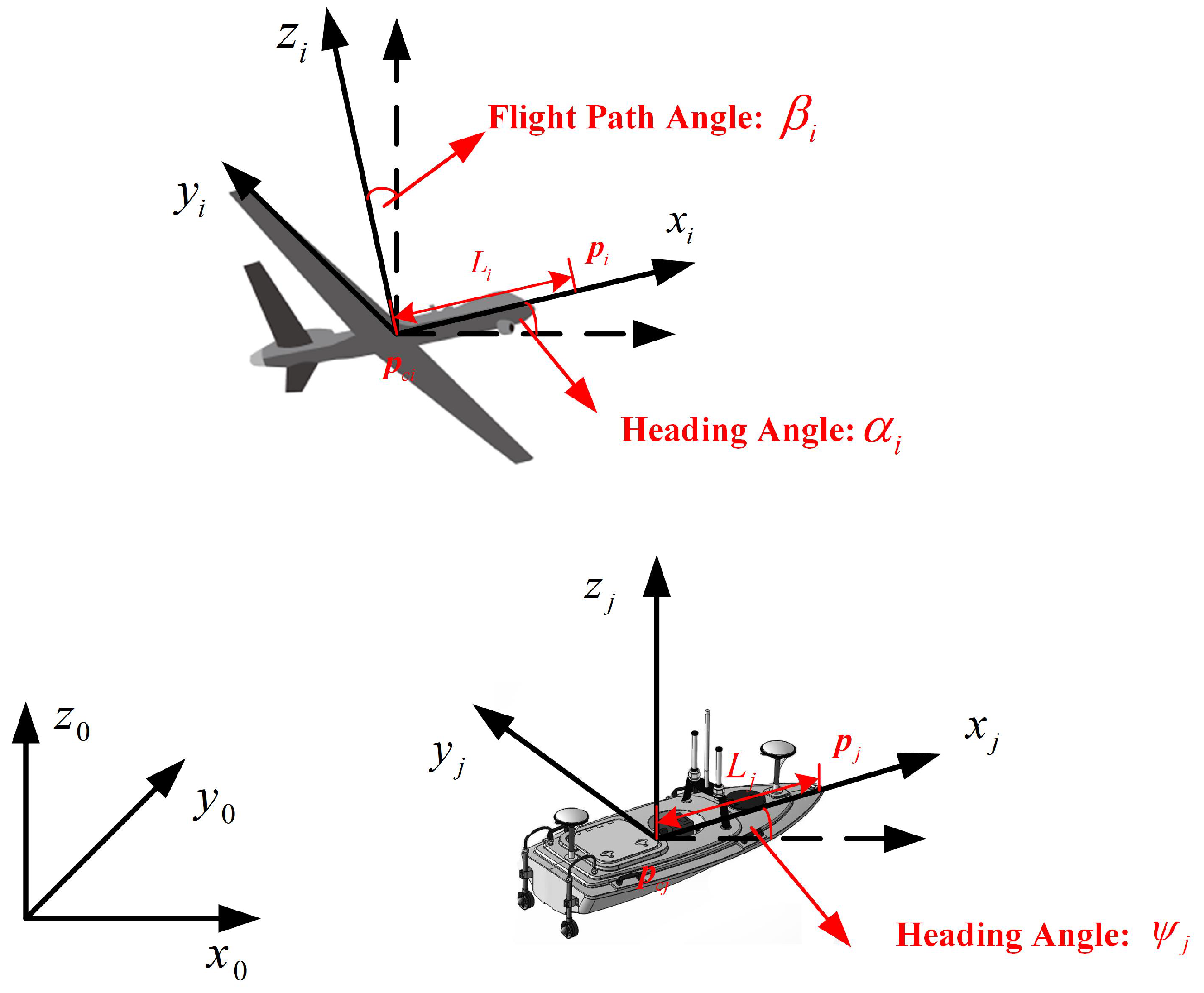
This paper investigates the formation control problem of UAV-UWSV heterogeneous multiagent system, and thus we only consider the kinematic models of UAVs and UWSVs that are selected from [30,31]. As shown in Figure 1, $\left\{O_0-x_0{y}_0{z}_0\right\}$ is the earth-fixed coordinate frame, and $\left\{O_i-x_i{y}_i{z}_i\right\}$ is the body-fixed coordinate frame of the ith agent.

2.1.1. UAV Model

The fixed-wing UAV is employed in our heterogeneous system, and the kinematics are described as [27].

$$\left\{\begin{array}{c}{\dot{x}}_{ci}=v_{i}cos{\beta }_{i}cos{\alpha }_i\hfill \\ {\dot{y}}_{ci}=v_{i}cos{\beta }_{i}sin{\alpha }_i\hfill \\ {\dot{z}}_{ci}=-v_{i}sin{\beta }_i\hfill \\ {\dot{\alpha }}_i={\omega }_{{\alpha }_i}\hfill \\ {\dot{\beta }}_i={\omega }_{{\beta }_i}\hfill \end{array}\right.,$$

(1)

where ${\mathit{p}}_{ci}={\left[x_{ci},y_{ci},z_{ci}\right]}^T$ is the position coordinate of the mass center of ith-UAV, ${\alpha }_i$ and ${\beta }_i$ represent the heading angle and flight path angle, $v_i$ is the airspeed and ${\omega }_{\alpha i}$ and ${\omega }_{\beta i}$ are the angular rates. Inspired by [31,32], the following coordinate transformation is performed, as shown in Figure 1. The hand position ${\mathit{p}}_i={\left[x_i,y_i,z_i\right]}^T$ is at a distance $L_i$ from the center of mass ${\mathit{p}}_{ci}$, as defined below.

$${\mathit{p}}_i={\left[x_{ci},y_{ci},z_{ci}\right]}^T+L_i{\left[c{\beta }_{i}c{\alpha }_i,c{\beta }_{i}s{\alpha }_i,-s{\beta }_i\right]}^T,$$

(2)

where $c{\alpha }_i\stackrel{\Delta }{=}cos{\alpha }_i$, $s{\alpha }_i\stackrel{\Delta }{=}sin{\alpha }_i$, respectively. Then, we have

$$\dot{{\mathit{p}}_i}=\left[\begin{array}{ccc}c{\beta }_{i}c{\alpha }_i& -L_{i}c{\beta }_{i}s{\alpha }_i& -L_{i}s{\beta }_{i}c{\alpha }_i\\ c{\beta }_{i}s{\alpha }_i& L_{i}c{\beta }_{i}c{\alpha }_i& -L_{i}s{\beta }_{i}s{\alpha }_i\\ -s{\beta }_i& 0& -L_{i}c{\beta }_i\end{array}\right]{\mathit{\eta }}_i,$$

(3)

where ${\mathit{\eta }}_i={\left[v_i,{\omega }_{{\alpha }_i},{\omega }_{{\beta }_i}\right]}^T$. By inversion, one has ${\mathit{\eta }}_i={\mathit{J}}_i\dot{{\mathit{p}}_i}$, where

$${\mathit{J}}_i=\left[\begin{array}{ccc}c{\beta }_{i}c{\alpha }_i& c{\beta }_{i}s{\alpha }_i& s{\beta }_i\\ -s{\alpha }_i/L_{i}c{\beta }_i& c{\alpha }_i/L_{i}c{\beta }_i& 0\\ -s{\beta }_{i}c{\alpha }_i/L_i& -s{\beta }_{i}s{\alpha }_i/L_i& c{\beta }_i/L_i\end{array}\right].$$

(4)

2.1.2. UWSV Model

For the sake of simplicity, we assume that the UWSVs in this research is fully actuated, i.e., the UWSVs can be individually controlled in heave, sway and spin directions. The kinematic model of jth-UWSV is described as follows [28]

$$\left\{\begin{array}{c}{\dot{x}}_{cj}=u_{j}cos{\psi }_j-v_{j}sin{\psi }_j\hfill \\ {\dot{y}}_{cj}=u_{j}sin{\psi }_j+v_{j}cos{\psi }_j\hfill \\ {\dot{\psi }}_j={\omega }_{{\psi }_j}\hfill \end{array}\right.,$$

(5)

where ${\mathit{p}}_{cj}={\left[x_{cj},y_{cj},0\right]}^T$ is the position coordinate of the mass center of jth-UWSV. Since UWSVs can only maneuver over the sea surface, we intentionally regulate the altitude of UWSVs as zero. $u_j$, $v_j$ and ${\omega }_{\psi j}$ are the surge, sway and yaw angular velocity, respectively.

Similarly, with the hand position ${\mathit{p}}_j={\left[x_j,y_j,0\right]}^T={\mathit{p}}_{cj}+L_j{\left[c{\psi }_j,s{\psi }_j,0\right]}^T$ at a distance $L_j$ from the center of mass ${\mathit{p}}_{cj}$, we have

$$\dot{{\mathit{p}}_j}=\left[\begin{array}{ccc}c{\psi }_j& -s{\psi }_j& -L_{j}s{\psi }_j\\ s{\psi }_j& c{\psi }_j& L_{j}c{\psi }_j\\ 0& 0& 0\end{array}\right]{\mathit{\eta }}_j,$$

(6)

where ${\mathit{\eta }}_j={\left[u_j,v_j,{\omega }_{{\psi }_j}\right]}^T$. By inversion, we have ${\mathit{\eta }}_j={\mathit{J}}_j\dot{{\mathit{p}}_j}$ with

$${\mathit{J}}_j=\left[\begin{array}{ccc}c{\psi }_j& s{\psi }_j& 0\\ s{\psi }_j/\phantom{-s{\psi }_j\left(L_j^2+1\right)}\left(L_j^2+1\right)& c{\psi }_j/\phantom{c{\psi }_j\left(L_j^2+1\right)}\left(L_j^2+1\right)& 0\\ -L_{j}s{\psi }_j/\phantom{-L_{j}s{\psi }_j\left(L_j^2+1\right)}\left(L_j^2+1\right)& L_{j}c{\psi }_j/\phantom{L_{j}c{\psi }_j\left(L_j^2+1\right)}\left(L_j^2+1\right)& 0\end{array}\right].$$

(7)

2.2. Heterogeneous Leader-First Follower Formation

Consider a UAV-UWSV heterogeneous multiagent system with m UAVs and n UWSVs. The communication and sensing graph of the system can be described by a directed graph $\mathcal{G}=\left\{\mathcal{V},\mathcal{E}\right\}$, where $\mathcal{V}=\left\{v_1,v_2,\cdots ,v_{m+n}\right\}$ is a vertex set with $\left|\mathcal{V}\right|=m+n$ and $\mathcal{E}=\left\{e_{ij}=\left(v_i,v_j\right)|v_i,v_j\in \mathcal{V},v_i\ne v_j\right\}$ is an edge set. If there exists $e_{ij}\in \mathcal{E}$ from $v_i$ to $v_j$, $v_j$ is called a neighbor vertex of $v_i$ and the neighbor set of $v_i$ is represented as ${\mathcal{N}}_i:=\left\{v_j\in \mathcal{V}|e_{ij}\in \mathcal{E}\right\}$.

We associate each vertex $v_i\in \mathcal{V}$ with the position of the ith vehicle (including both UAVs and UWSVs). If a directed edge $e_{ij}$ exists, agent i can receive information from agent j. The stacked vector $\mathit{p}={\left[{\mathit{p}}_1^T,\cdots ,{\mathit{p}}_{m+n}^T\right]}^T\in {\mathbb{R}}^{3(m+n)}$ is referred to as a configuration of $\mathcal{G}$. The formation $\mathcal{G}\left(\mathit{p}\right)$ is defined with the directed graph $\mathcal{G}$ and the configuration $\mathit{p}$ [33]. With ${\mathit{z}}_{ij}={\mathit{p}}_j-{\mathit{p}}_i$ as the displacement vector of ${\mathit{p}}_i$ and ${\mathit{p}}_j$, the distance of ${\mathit{p}}_i$ and ${\mathit{p}}_j$ is defined as $d_{ij}=∥{\mathit{z}}_{ij}∥$. The bearing vector ${\mathit{g}}_{ij}$ is defined as the unit vector from ${\mathit{p}}_i$ to ${\mathit{p}}_j$ as shown below

$${\mathit{g}}_{ij}=\frac{{\mathit{p}}_i-{\mathit{p}}_j}{∥{\mathit{p}}_i-{\mathit{p}}_j∥}=\frac{{\mathit{z}}_{ij}}{∥{\mathit{z}}_{ij}∥}.$$

(8)

Unlike position-based formation control approaches [13,14,15,16,17,18], in which every vehicle has access to its global position, bearing-based approaches require each agent to maintain one or several bearing vectors with its neighbors, which makes the uniqueness of the bearing-based formation a fundamental problem. Obviously, it is unnecessary to control all bearing vectors to maintain a target formation. According to the bearing rigidity theory proposed in [21], the target formation is achieved if a specific subset of desired bearing vectors is attained in an undirected graph. In practice, it is difficult to guarantee the agents can communicate with each other directly, whereas the uniqueness of the bearing-based formation in directed graphs remains unsolved so far. As a primary study, [26] discussed the uniqueness of the bearing-based formation in a certain class of directed graph named LFF graph under the following assumption.

Assumption 1

([26]). The target formation is characterized by a set of desired constant bearing constraints $B=\left\{{\mathit{g}}_{ij}^{*}|e_{ij}\in \mathcal{E}\right\}$ with the following conditions: (1) The target bearing constraints are achievable. In other words, there exists a configuration $\tilde{\mathit{p}}$ such that ${\mathit{g}}_{ij}^{*}=\frac{{\tilde{\mathit{p}}}_j-{\tilde{\mathit{p}}}_i}{∥{\tilde{\mathit{p}}}_j-{\tilde{\mathit{p}}}_i∥}$. (2) For agent $v_i$ ($i\ge 3$), the desired bearing vectors to its two neighbors $v_j$ and $v_k$ are not co-linear, i.e., ${\mathit{g}}_{ij}^{*}={\mathit{g}}_{ik}^{*}$.

With this assumption, the definition of LFF graph is given as follows.

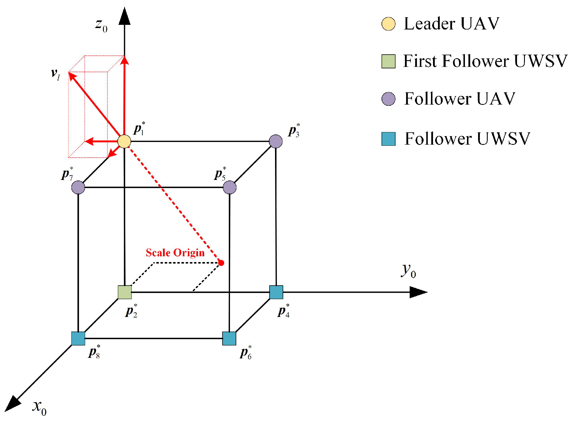
Definition 1.

(LFF Graph) [26] A LFF graph $\mathcal{G}=\left(\mathcal{V},\mathcal{E}\right)$ is an acyclic and rooted in-branching directed graph with n vertices ($n\ge 3$) and $2n-3$ well-selected directed edges. The n vertices are composed of one leader vertex $v_1$, one first follower vertex $v_2$ and $n-2$ follower vertices $\left\{v_3,\cdots ,v_n\right\}$. The $2n-3$ directed edges consist of one from the first follower vertex to the leader vertex and two for each follower vertex.

Inspired by the above study, we extend the LFF graph to a heterogeneous multiagent system and propose a heterogeneous leader-first follower (HLFF) formation. With the above assumption, the definition of an HLFF graph for m UAVs and n UWSVs is given as follows.

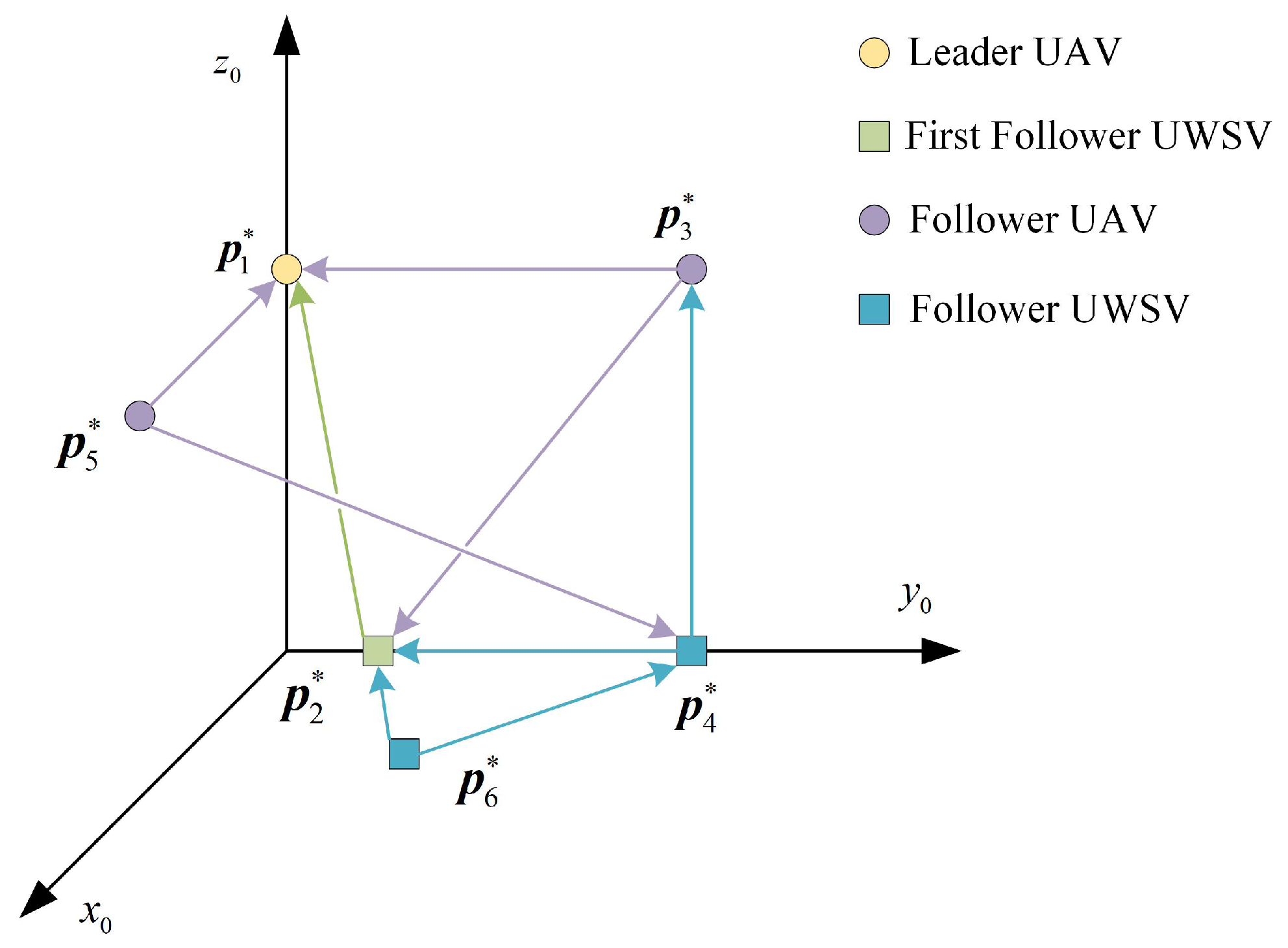
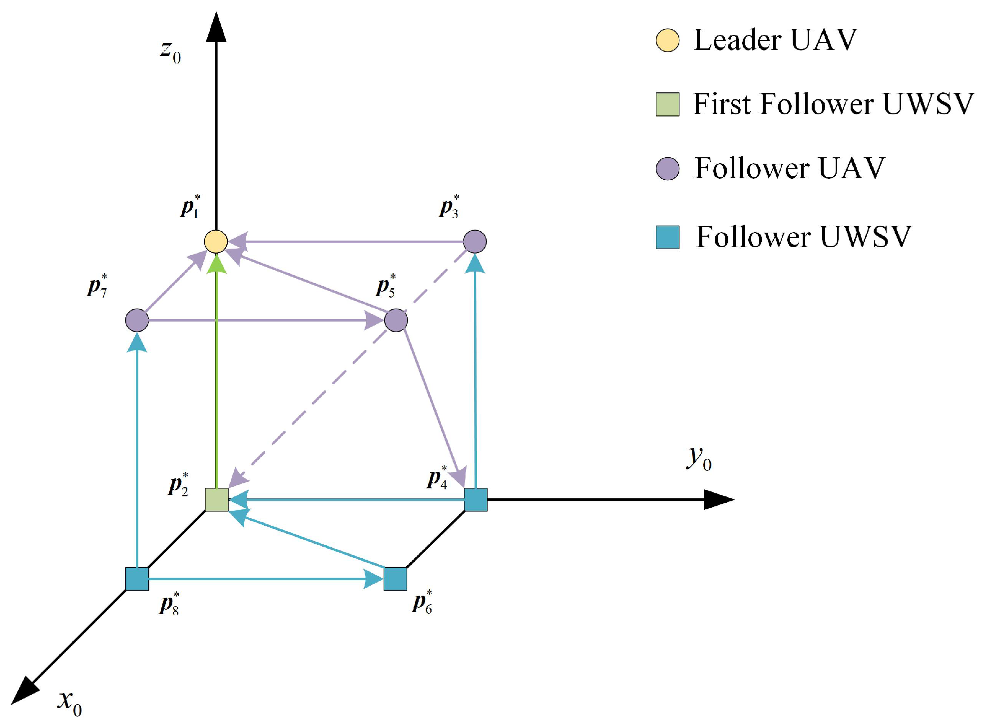
Definition 2.

(HLFF Graph) An HLFF graph $\mathcal{G}=\left(\mathcal{V},\mathcal{E}\right)$ is an acyclic and rooted in-branching directed graph with m UAV vertices, n UWSV vertices and $2(m+n)-3$ well-selected directed edges. The $m+n$ vertices are composed of one leader UAV vertex $v_1$, one first follower UWSV vertex and $v_1$ and $m+n-2$ follower vertices $\left\{v_2,\cdots ,v_{m+n}\right\}$. The $2(m+n)-3$ directed edges consist of one from the first follower UWSV vertex to the leader UAV vertex and two for each other follower vertices.

Remark 1.

The LFF graph concentrates on homogeneous systems, and, therefore, it cannot be applied directly to a mixed-order heterogeneous system such as the UAV-UWSV system. That is because the UWSVs can measure the three-dimensional (3D) bearing vector between UWSV and UAV, but they can only maneuver in the two-dimensional (2D) plane to achieve the 3D formation. However, in the LFF graph, it is assumed that all agents can move in the same dimensional space.

Without loss of generality, let leader vertex $v_1$ represent the position of the leader UAV, vertex $v_2$ represents the position of the first follower UWSV, vertex $v_i$$(i\ge 3)$ represents the position of the ith-UAV or UWSV. $v_2$ has only one directed edge $e_{ij}$, which means it can measure the relative bearing vector ${\mathit{g}}_{ij}$ from the leader UAV. Each follower agent has two directed edges to receive information from its neighbors. An example of an HLFF graph with three UAVs and three UWSVs is shown in Figure 2.

2.3. Properties of HLFF Graph

This section discusses some properties of HLFF graphs, including the uniqueness of the HLFF graph and the translational and scaling motion of the HLFF graph.

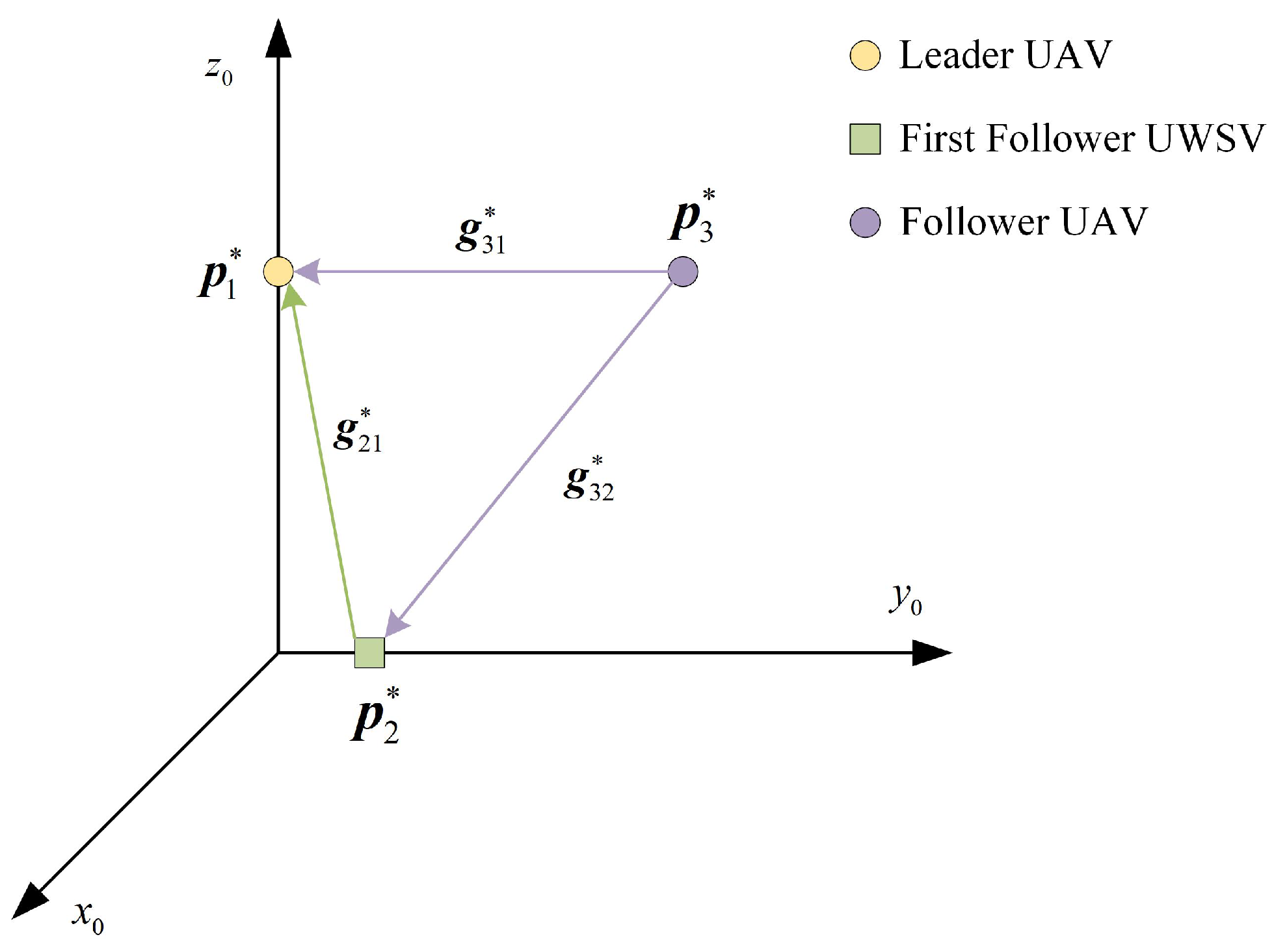
Lemma 1.

(Uniqueness of HLFF graph) Consider a UAV-UWSV heterogeneous multiagent system with an HLFF graph. Under Assumption 1, given the position of the leader UAV ${\mathit{p}}_1^{*}$ and a set of desired bearing constraints $B=\left\{{\mathit{g}}_{ij}^{*}|e_{ij}\in \mathcal{E}\right\}$, then, the desired formation $\mathcal{G}\left({\mathit{p}}^{*}\right)$ with ${\mathit{p}}^{*}={\left[{\mathit{p}}_1^{*T},{\mathit{p}}_2^{*T},\dots ,{\mathit{p}}_{m+n}^{*T}\right]}^T$ is uniquely determined.

Proof. 

As shown in Figure 3, $\theta$ is the angle between ${\mathit{g}}_{21}^{*}$ and axis $z_0$. In triangle ${\mathit{p}}_1^{*}{O}_0{\mathit{p}}_2^{*}$, the relative position between ${\mathit{p}}_1^{*}$ and ${\mathit{p}}_2^{*}$ can be obtained according to trigonometric geometry

$${\mathit{p}}_2^{*}={\left[{\left({\mathit{p}}_1^{*}\right)}_x,{\left({\mathit{p}}_1^{*}\right)}_y,0\right]}^T+{\left[\frac{{\left({\mathit{p}}_1^{*}\right)}_z{\left({\mathit{g}}_{21}^{*}\right)}_x}{{\left({\mathit{g}}_{21}^{*}\right)}_z},\frac{{\left({\mathit{p}}_1^{*}\right)}_z{\left({\mathit{g}}_{21}^{*}\right)}_y}{{\left({\mathit{g}}_{21}^{*}\right)}_z},0\right]}^T,$$

(9)

where ${\left({\mathit{g}}_{21}^{*}\right)}_k$ is the component of ${\mathit{g}}_{21}^{*}$ on the k-axis ($k=x,y,z$).

For the third agent, the position ${\mathit{p}}_3^{*}$ satisfies two bearing vectors ${\mathit{g}}_{31}^{*}$ and ${\mathit{g}}_{32}^{*}$, as shown in Figure 3. Thus,

$$\begin{array}{c}{\mathit{P}}_{{\mathit{g}}_{31}^{*}}\left({\mathit{p}}_1^{*}-{\mathit{p}}_3^{*}\right)=\mathbf{0}\\ {\mathit{P}}_{{\mathit{g}}_{32}^{*}}\left({\mathit{p}}_2^{*}-{\mathit{p}}_3^{*}\right)=\mathbf{0},\end{array}$$

(10)

where ${\mathit{P}}_{{\mathit{g}}_{ij}^{*}}=\mathit{I}-{\mathit{g}}_{ij}^{*}{\left({\mathit{g}}_{ij}^{*}\right)}^T$ is the orthogonal projection matrix of ${\mathit{g}}_{ij}^{*}$.

From (10), it follows that

$$\left({\mathit{P}}_{{\mathit{g}}_{31}^{*}}+{\mathit{P}}_{{\mathit{g}}_{32}^{*}}\right){\mathit{p}}_3^{*}={\mathit{P}}_{{\mathit{g}}_{31}^{*}}{\mathit{p}}_1^{*}+{\mathit{P}}_{{\mathit{g}}_{32}^{*}}{\mathit{p}}_2^{*}.$$

(11)

For $\left({\mathit{P}}_{{\mathit{g}}_{31}^{*}}+{\mathit{P}}_{{\mathit{g}}_{32}^{*}}\right)$, we have $Null\left({\mathit{P}}_{{\mathit{g}}_{31}^{*}}\right)=span\left({\mathit{g}}_{31}^{*}\right)$ and $Null\left({\mathit{P}}_{{\mathit{g}}_{32}^{*}}\right)=span\left({\mathit{g}}_{32}^{*}\right)$. As ${\mathit{g}}_{31}^{*}\ne \pm {\mathit{g}}_{32}^{*}$ exists under Assumption 1, and ${\mathit{P}}_{g_{31}^{*}}$, ${\mathit{P}}_{g_{32}^{*}}$ are positive semidefinite matrices; we have $Null\left({\mathit{P}}_{{\mathit{g}}_{31}^{*}}\right)\cap Null\left({\mathit{P}}_{{\mathit{g}}_{32}^{*}}\right)=\left\{\mathbf{0}\right\}$. Therefore, $\left({\mathit{P}}_{{\mathit{g}}_{31}^{*}}+{\mathit{P}}_{{\mathit{g}}_{32}^{*}}\right)$ is non-singular and ${\mathit{p}}_3^{*}$ can be obtained by

$${\mathit{p}}_3^{*}={\left({\mathit{P}}_{{\mathit{g}}_{31}^{*}}+{\mathit{P}}_{{\mathit{g}}_{32}^{*}}\right)}^{-1}\left({\mathit{P}}_{{\mathit{g}}_{31}^{*}}{\mathit{p}}_1^{*}+{\mathit{P}}_{{\mathit{g}}_{32}^{*}}{\mathit{p}}_2^{*}\right).$$

(12)

Similarly, for $i=4,\dots ,n+m$, the desired position can be iteratively calculated as

$${\mathit{p}}_i^{*}={\left({\mathit{P}}_{{\mathit{g}}_{ij}^{*}}+{\mathit{P}}_{{\mathit{g}}_{ik}^{*}}\right)}^{-1}\left({\mathit{P}}_{{\mathit{g}}_{ij}^{*}}{\mathit{p}}_i^{*}+{\mathit{P}}_{{\mathit{g}}_{ik}^{*}}{\mathit{p}}_k^{*}\right).$$

(13)

Thus, given the desired bearing constraints B and the position of leader UAV ${\mathit{p}}_1^{*}$, the HLLF formation can be uniquely determined. □

To describe the translation and scaling of the HLFF graph, we introduce the centroid $c\left({\mathit{p}}^{*}\left(t\right)\right)$ and scale $s\left({\mathit{p}}^{*}\left(t\right)\right)$ of the HLFF graph as follows.

$$\left\{\begin{array}{c}c\left({\mathit{p}}^{*}\left(t\right)\right)=\frac{1}{n}{\displaystyle \sum _{i=1}^n}{\mathit{p}}_i^{*}\left(t\right)\hfill \\ s\left({\mathit{p}}^{*}\left(t\right)\right)=\sqrt{\frac{1}{n}{\displaystyle \sum _{i=1}^n}{∥{\mathit{p}}_i^{*}\left(t\right)-c\left({\mathit{p}}^{*}\left(t\right)\right)∥}^2}\hfill \end{array}\right.$$

(14)

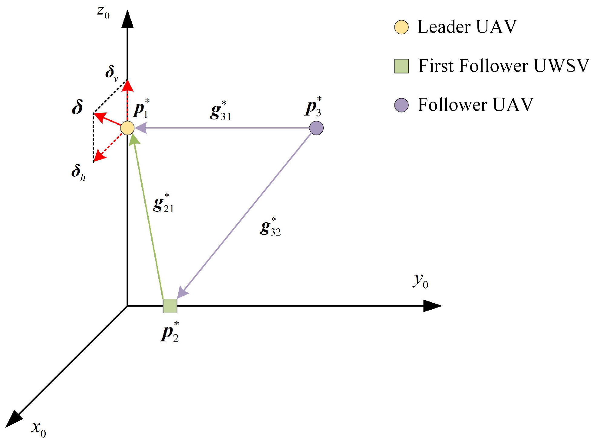
Lemma 2.

(Translation and scale of HLFF graph) For an HLFF graph, given a set of bearing vectors $\left\{{\mathit{g}}_{ij}^{*}\right\}$$(\left(i,j\right)\in \mathcal{E})$, the translation of the entire formation is determined by the leader UAV’s horizontal motion and the scale of the entire formation is determined by the leader UAV’s vertical motion.

Proof. 

Similar to Lemma 1, we consider the HLFF graph shown in Figure 3. Consider the leader UAV moves from ${\mathit{p}}_1^{*}$ to ${\mathit{q}}_1^{*}={\mathit{p}}_1^{*}+\delta$; the motion process $\delta$ can be decomposed into two individual motion: horizontal motion ${\delta }_h={\left[{\delta }_x,{\delta }_y,0\right]}^T$ and vertical motion ${\delta }_v={\left[0,0,{\delta }_z\right]}^T$, as shown in Figure 4.

If the leader UAV only has horizontal motion ${\left({\mathit{p}}_1^{*}\right)}_h={\mathit{p}}_1^{*}+{\delta }_h$, we only need to prove that each follower has ${\left({\mathit{p}}_i^{*}\right)}_h={\mathit{p}}_i^{*}+{\delta }_h$. For the first follower UWSV, according to (9), we have

$${\left({\mathit{p}}_2^{*}\right)}_h={\left[{\left({\mathit{p}}_1^{*}\right)}_x,{\left({\mathit{p}}_1^{*}\right)}_y,0\right]}^T+{\delta }_h+{\left[\frac{{\left({\left({\mathit{p}}_1^{*}\right)}_h\right)}_z{\left({\mathit{g}}_{21}^{*}\right)}_x}{{\left({\mathit{g}}_{21}^{*}\right)}_z},\frac{{\left({\left({\mathit{p}}_1^{*}\right)}_h\right)}_z{\left({\mathit{g}}_{21}^{*}\right)}_y}{{\left({\mathit{g}}_{21}^{*}\right)}_z},0\right]}^T.$$

(15)

As ${\left({\left({\mathit{p}}_1^{*}\right)}_h\right)}_z={\left({\mathit{p}}_1^{*}\right)}_z$, we have ${\left({\mathit{p}}_2^{*}\right)}_h={\mathit{p}}_2^{*}+{\delta }_h$. For the UAV follower 3, we have

$$\begin{array}{cc}\hfill {\left({\mathit{p}}_3^{*}\right)}_h& ={\left({\mathit{P}}_{{\mathit{g}}_{31}^{*}}+{\mathit{P}}_{{\mathit{g}}_{32}^{*}}\right)}^{-1}\left({\mathit{P}}_{{\mathit{g}}_{31}^{*}}{\left({\mathit{p}}_1^{*}\right)}_h+{\mathit{P}}_{{\mathit{g}}_{32}^{*}}{\left({\mathit{p}}_2^{*}\right)}_h\right)\hfill \\ \hfill & ={\left({\mathit{P}}_{{\mathit{g}}_{31}^{*}}+{\mathit{P}}_{{\mathit{g}}_{32}^{*}}\right)}^{-1}\left({\mathit{P}}_{{\mathit{g}}_{31}^{*}}{\mathit{p}}_1^{*}+{\mathit{P}}_{{\mathit{g}}_{32}^{*}}{\mathit{p}}_2^{*}+\left({\mathit{P}}_{{\mathit{g}}_{31}^{*}}+{\mathit{P}}_{{\mathit{g}}_{32}^{*}}\right){\delta }_h\right)\hfill \\ \hfill & ={\mathit{p}}_3^{*}+{\delta }_h.\hfill \end{array}$$

(16)

The proof for $i\ge 4$ can follow the same pattern as follower 3. According to (14), we have $c\left({\left({\mathit{p}}^{*}\right)}_h\right)=c\left({\mathit{p}}^{*}\right)+{\delta }_h$, which means that the translation of the formation can be controlled by the horizontal motion of the leader UAV.

If the leader UAV only has vertical motion ${\left({\mathit{p}}_1^{*}\right)}_v={\mathit{p}}_1^{*}+{\delta }_v$, we assume that ${\left({\left({\mathit{p}}_1^{*}\right)}_v\right)}_z=\beta {\left({\mathit{p}}_1^{*}\right)}_z$. For first follower UWSV, we have $∥{\left({\mathit{p}}_1^{*}\right)}_v-{\left({\mathit{p}}_2^{*}\right)}_v∥=\beta ∥{\mathit{p}}_1^{*}-{\mathit{p}}_2^{*}∥$ according to trigonometry.

With (9), it can be obtained that

$$∥{\left({\mathit{p}}_1^{*}\right)}_v-{\left({\mathit{p}}_2^{*}\right)}_v∥=\beta \frac{\sqrt{{\left({\left({\mathit{g}}_{12}^{*}\right)}_x\right)}^2+{\left({\left({\mathit{g}}_{12}^{*}\right)}_y\right)}^2}}{\left|{\left({\mathit{g}}_{12}^{*}\right)}_x\right|}\left|{\left({\mathit{p}}_1^{*}\right)}_z\right|.$$

(17)

Therefore, we have $∥{\left({\mathit{p}}_1^{*}\right)}_v-{\left({\mathit{p}}_2^{*}\right)}_v∥\propto \left|{\left({\mathit{p}}_1^{*}\right)}_z\right|$. For the UAV follower 3, we have

$$\begin{array}{cc}\hfill {\left({\mathit{p}}_1^{*}\right)}_v-{\left({\mathit{p}}_3^{*}\right)}_v& ={\left({\mathit{p}}_1^{*}\right)}_v-{\left({\mathit{P}}_{{\mathit{g}}_{31}^{*}}+{\mathit{P}}_{{\mathit{g}}_{32}^{*}}\right)}^{-1}\left({\mathit{P}}_{{\mathit{g}}_{31}^{*}}{\left({\mathit{p}}_1^{*}\right)}_v+{\mathit{P}}_{{\mathit{g}}_{32}^{*}}{\left({\mathit{p}}_2^{*}\right)}_v\right)\hfill \\ \hfill & ={\left({\mathit{P}}_{{\mathit{g}}_{31}^{*}}+{\mathit{P}}_{{\mathit{g}}_{32}^{*}}\right)}^{-1}\left(\left({\mathit{P}}_{{\mathit{g}}_{31}^{*}}+{\mathit{P}}_{{\mathit{g}}_{32}^{*}}\right){\left({\mathit{p}}_1^{*}\right)}_v-{\mathit{P}}_{{\mathit{g}}_{31}^{*}}{\left({\mathit{p}}_1^{*}\right)}_v-{\mathit{P}}_{{\mathit{g}}_{32}^{*}}{\left({\mathit{p}}_2^{*}\right)}_v\right)\hfill \\ \hfill & ={\left({\mathit{P}}_{{\mathit{g}}_{31}^{*}}+{\mathit{P}}_{{\mathit{g}}_{32}^{*}}\right)}^{-1}{\mathit{P}}_{{\mathit{g}}_{32}^{*}}\left({\left({\mathit{p}}_1^{*}\right)}_v-{\left({\mathit{p}}_2^{*}\right)}_v\right).\hfill \end{array}$$

(18)

Thus, $∥{\left({\mathit{p}}_1^{*}\right)}_v-{\left({\mathit{p}}_3^{*}\right)}_v∥\propto ∥{\left({\mathit{p}}_1^{*}\right)}_v-{\left({\mathit{p}}_2^{*}\right)}_v∥\propto \left|{\left({\mathit{p}}_1^{*}\right)}_z\right|$.

Similarly, it can be seen that $\forall \left(v_i,v_j\right)\in \mathcal{E}$, $∥{\left({\mathit{p}}_i^{*}\right)}_v-{\left({\mathit{p}}_j^{*}\right)}_v∥=\beta ∥{\mathit{p}}_i^{*}-{\mathit{p}}_j^{*}∥$. Since the HLFF graph can be generated via the bearing-based Henneberg construction; it has a spanning tree [27]. $\forall v_i\in \mathcal{V}$, there exists a finite path $\left(v_{i0},v_{i1}\right)$, $\left(v_{i1},v_{i2}\right)$, ⋯, $\left(v_{i(k-1)},v_{ik}\right)$ that $v_{i0}=v_1,v_{ik}=v_i$. Then we have

$${\left({\mathit{p}}_1^{*}\right)}_v-{\left({\mathit{p}}_i^{*}\right)}_v=\sum _{j=1}^k\left({\left({\mathit{p}}_{i(j-1)}^{*}\right)}_v-{\left({\mathit{p}}_{ij}^{*}\right)}_v\right)=\sum _{j=1}^k\beta \left({\mathit{p}}_{i(j-1)}^{*}-{\mathit{p}}_{ij}^{*}\right)=\beta \left({\mathit{p}}_1^{*}-{\mathit{p}}_i^{*}\right)$$

(19)

Furthermore, it can be deduced that $\forall v_i\in \mathcal{V}$, $∥{\left({\mathit{p}}_i^{*}\right)}_v-{\left({\mathit{p}}_j^{*}\right)}_v∥=\beta ∥{\mathit{p}}_i^{*}-{\mathit{p}}_j^{*}∥$. Therefore, we conclude that

$$∥{\left({\mathit{p}}_i^{*}\right)}_v-c\left({\left({\mathit{p}}^{*}\right)}_v\right)∥=\frac{1}{n}\sum _{j=1}^n∥{\left({\mathit{p}}_i^{*}\right)}_v-{\left({\mathit{p}}_j^{*}\right)}_v∥=\beta ∥{\mathit{p}}_i^{*}-c\left({\mathit{p}}^{*}\right)∥$$

(20)

Equivalently, we have $s\left({\left({\mathit{p}}^{*}\right)}_v\right)=\beta s\left({\mathit{p}}^{*}\right)$, which means the scale of the HLFF graph can be controlled by the vertical motion of the leader UAV. □

Remark 2.

From [25], it can be seen that LFF graph is not bearing-only, because it needs to measure the distance between the leader and the first follower accurately to control the scale of the formation, which still retains the disadvantage of distance measurement in the practical perspective. However, the HLFF graph does not need any distance measurement, which makes it a bearing-only method.

Remark 3.

The LFF graph needs the first follower to actively measure its distance and bearing vector from the leader to find its global position, which can be seen as a two-leader control scheme as the scaling of the formation cannot be controlled by the leader individually. However, in the HLFF graph, both translation and scaling of the formation can be controlled by the leader, which makes it a single-leader control scheme. Therefore, the HLFF graph reduces the parameters required for the formation maneuver.

2.4. Problem Formulation

Before the problem is formulated, we assume that the UAV-UWSV heterogeneous multiagent system satisfies the following assumptions:

Assumption 2.

The communication graph of the system is characterized by a directed graph $\mathcal{G}=\left(\mathcal{V},\mathcal{E}\right)$ with an HLFF structure.

Assumption 3.

The initial positions of all agents are not collocated, i.e., ${\mathit{p}}_i\left(0\right)\ne {\mathit{p}}_j\left(0\right)$ ($\forall 1\le i\ne j\le m+n$).

Assumption 2 guarantees that the desired formation is uniquely determined given a set of achievable bearing vectors $\left\{{\mathit{g}}_{ij}^{*}\right\}$, and the translation and the scale of the formation can be regulated by the leader UAV ${{\ddot{\mathit{p}}}_1}^{*}$.

Assumption 4.

The leader UAV satisfies ${\mathit{p}}_1\left(t\right)={\mathit{p}}_1^{*}\left(t\right),\forall t>0$, and there exists a positive constant ${\delta }_L$ such that ${∥{\ddot{\mathit{p}}}_1∥}_1\le {\delta }_L<+\infty$, that is, the acceleration of the leader is bounded.

In this paper, assuming the leader UAV moves along a predefined trajectory, we do not consider its motion control. For the sake of simplicity, we assume that there is no internal failure or external disturbance, such as potential obstacles or disruptions during the formation maneuver. With Assumption 4 and (13), we have $∥{\ddot{\mathit{p}}}_i^{*}∥\le {\delta }_L$ ($2\le i\le m+n$). Under the above assumptions, our problem is formulated as follows.

Problem 1.

Consider a UAV-UWSV heterogeneous multiagent system with m UAVs and n UWSVs, under Assumptions 1–4, using only relative bearing measurements and local interactions, design distributed control law for ${\mathit{\eta }}_i$ such that i ($2\le i\le m+n$) such that ${\mathit{g}}_{ij}\left(t\right)$ converges to ${\mathit{g}}_{ij}^{*}$ asymptotically as $t\to \infty$.

3. Bearing-Only Formation Control Scheme

In this section, we propose a hierarchical bearing-only formation protocol for UAV-UWSV heterogeneous multiagent system. Specifically, we first propose a finite-time distributed observer for each follower to estimate the reference velocity. Secondly, on the basis of estimated reference and relative bearing measurements, a bearing-only formation control law is designed to achieve the target formation. The control scheme is shown in Figure 5.

3.1. Finite-time Distributed Observer Design

Because the first follower can receive the information from the leader UAV directly, as illustrated in Figure 3, the reference velocity of the first follower UWSV ${\mathit{p}}_2$ can be calculated as

$${\mathit{r}}_2={\left[{\left({\dot{\mathit{p}}}_1^{*}\right)}_x,{\left({\dot{\mathit{p}}}_1^{*}\right)}_y,0\right]}^T+{\left[\frac{{\left({\dot{\mathit{p}}}_1^{*}\right)}_z{\left({\mathit{g}}_{21}^{*}\right)}_x}{{\left({\mathit{g}}_{21}^{*}\right)}_z},\frac{{\left({\dot{\mathit{p}}}_1^{*}\right)}_z{\left({\mathit{g}}_{21}^{*}\right)}_y}{{\left({\mathit{g}}_{21}^{*}\right)}_z},0\right]}^T.$$

(21)

For the ith-follower $(i\ge 3)$, the distributed observer is designed as follows.

$${\dot{\mathit{r}}}_i=-\beta \mathrm{sgn}\left({\mathit{P}}_{{\mathit{g}}_{ij}^{*}}\left({\mathit{r}}_i-{\mathit{r}}_j\right)+{\mathit{P}}_{{\mathit{g}}_{ik}^{*}}\left({\mathit{r}}_i-{\mathit{r}}_k\right)\right),$$

(22)

where ${\mathit{r}}_i$ is the estimation of ${\dot{\mathit{p}}}_i$, $\beta$ is a positive constant to be determined, ${\mathit{r}}_1={\dot{\mathit{p}}}_1^{*}$. It can be observed that the velocity estimation of the ith-follower requires its neighbors’ velocity estimations ${\mathit{r}}_j$ and ${\mathit{r}}_k$.

Lemma 3.

Let $\beta >{\delta }_L$, under Assumptions 1–4 and the estimation law (22), ${\mathit{r}}_i\left(t\right)$ converges to ${\dot{\mathit{p}}}_i^{*}\left(t\right)$ in finite time, i.e., ${\mathit{r}}_i\left(t\right)={\dot{\mathit{p}}}_i^{*}\left(t\right)$ ($t\ge T_e$), where $T_e$ is a positive constant to be introduced later.

Proof. 

Let ${\tilde{\mathit{r}}}_i={\mathit{r}}_i-{\dot{\mathit{p}}}_i^{*}$ and define $\tilde{\mathit{r}}={\left[{{\tilde{\mathit{r}}}_3}^T,{{\tilde{\mathit{r}}}_4}^T\cdots ,{\tilde{\mathit{r}}}_{m+n}^T\right]}^T$ for convenience.

Before proceeding, we introduce a bearing Laplacian matrix $\mathit{B}$, which is defined as

$${\mathit{B}}_{ij}=\left\{\begin{array}{cc}\mathbf{0}\hfill & i\ne j,{\mathit{e}}_{ij}\notin \mathcal{E}\hfill \\ -{\mathit{P}}_{{\mathit{g}}_{ij}}\hfill & i\ne j,{\mathit{e}}_{ij}\in \mathcal{E}\hfill \\ {\displaystyle \sum _{v_k\in {\mathcal{N}}_i}}{\mathit{P}}_{{\mathit{g}}_{ik}}\hfill & i=j\hfill \end{array}\right.,$$

(23)

where ${\mathit{B}}_{ij}$ is the (i, j)th submatrix of $\mathit{B}$.

Considering the hierarchical structure of the HLFF graph, the leader has no neighbors. Therefore, the bearing Laplacian matrix can be partitioned as

$$\mathit{B}=\left[\begin{array}{ccc}\mathbf{0}& \mathbf{0}& \mathbf{0}\\ {\mathit{B}}_{2,1}& {\mathit{B}}_{2,2}& \mathbf{0}\\ {\mathit{B}}_{f,1}& {\mathit{B}}_{f,2}& {\mathit{B}}_{f,3}.\end{array}\right]$$

(24)

Note that ${\mathit{B}}_{f,3}$ is a lower triangular matrix; its eigenvalues are the eigenvalues of diagonal matrix $B_{i,i}$ ($i\ge 3$). Under the feasibility conditions of desired bearing vectors, ${\mathit{B}}_{i,i}$ is positive definite. Therefore, ${\mathit{B}}_{f,3}$ is positive definite [34].

Consider the Lyapunov function $V_e={\tilde{\mathit{r}}}^T{\mathit{B}}_{f,3}^T\tilde{\mathit{r}}/\phantom{{\tilde{\mathit{r}}}^T{\mathit{B}}_{f,3}^T\tilde{\mathit{r}}2}2$. The derivative can be obtained as

$$\begin{array}{cc}\hfill {\dot{V}}_e& ={\tilde{\mathit{r}}}^T{\mathit{B}}_{f,3}^T\left(-\beta \mathrm{sgn}\left({\mathit{B}}_{f,3}^T\tilde{\mathit{r}}\right)-{\ddot{\mathit{p}}}^{*}\right)\hfill \\ \hfill & \le -\left(\beta -{\delta }_L\right){∥{\mathit{B}}_{f,3}∥}_1{∥\tilde{\mathit{r}}∥}_1\hfill \\ \hfill & \le -\left(\beta -{\delta }_L\right){∥{\mathit{B}}_{f,3}∥}_1{∥\tilde{\mathit{r}}∥}_2\hfill \\ \hfill & \le -\sqrt{2}\frac{\left(\beta -{\delta }_L\right){∥{\mathit{B}}_{f,3}∥}_1}{\sqrt{{\lambda }_{max}\left({\mathit{B}}_{f,3}\right)}}{V}_e^{\frac{1}{2}}.\hfill \end{array}$$

(25)

Under Theorem 4.2 in [35], $\tilde{\mathit{r}}\to \mathbf{0}$ in a settling time $T_e=\frac{\sqrt{2{\lambda }_{max}\left({\mathit{B}}_{f,3}\right)}}{\left(\beta -{\delta }_L\right){∥{\mathit{B}}_{f,3}∥}_1}{V}_e^{\frac{1}{2}}$. □

3.2. Bearing-Only Formation Control Law Design

We now consider the case with $t\ge T_e$. The following bearing-only formation control law for the ith-follower is proposed as follows.

$${\mathit{\eta }}_i={\mathit{J}}_i\left(-c{\mathit{P}}_i\left(\sum _{j\in {\mathcal{N}}_i}{\mathit{P}}_{{\mathit{g}}_{ij}}{\mathit{g}}_{ij}^{*}\right)+{\mathit{r}}_i\right).$$

(26)

where c is a positive constant to be determined, and ${\mathit{P}}_i$ is the projection matrix with the following form:

$${\mathit{P}}_i=\left\{\begin{array}{cc}\mathit{I}-{\mathit{e}}_3{{\mathit{e}}_3}^T& i\in \mathrm{UWSV}\\ \mathit{I}& i\in \mathrm{UAV}\end{array}\right.,$$

(27)

where ${\mathit{e}}_3$ denotes the $i\mathrm{th}$ unit orthogonal base of ${\mathbb{R}}^3$.

Theorem 1.

Under Assumptions 1–4 and control law (26), ${\mathit{p}}_i\left(t\right)$ asymptotically converges to ${\mathit{p}}_i^{*}\left(t\right)$

Proof. 

For the first follower UWSV, as it only has the leader UAV as its neighbor, substituting the control law (26) into (6) yields

$${\dot{\mathit{p}}}_2=-c{\mathit{P}}_2{\mathit{P}}_{{\mathit{g}}_{ij}}{\mathit{g}}_{ij}^{*}+{\mathit{r}}_2.$$

(28)

From (28) and the properties of the orthogonal projection matrix, we have that ${\dot{\mathit{p}}}_2={\widehat{\mathit{r}}}_2$ if and only if ${\mathit{g}}_{21}={\mathit{g}}_{21}^{*}$.

Considering the Lyapunov function $V_2=\frac{1}{2}{∥{\mathit{p}}_2-{\mathit{p}}_2^{*}∥}^2$. The derivative of $V_b$ is

$$\begin{array}{cc}\hfill {\dot{V}}_2& ={\left({\mathit{p}}_2-{\mathit{p}}_2^{*}\right)}^T\left({\dot{\mathit{p}}}_2-{\dot{\mathit{p}}}_2^{*}\right)={\left({\mathit{p}}_2-{\mathit{p}}_2^{*}\right)}^T\left(-c{\mathit{P}}_2{\mathit{P}}_{{\mathit{g}}_{21}}{\mathit{g}}_{21}^{*}+{\widehat{\mathit{r}}}_2-{\dot{\mathit{p}}}_2^{*}\right)\hfill \\ \hfill & =-c{\mathit{P}}_2{\left({\mathit{p}}_2-{\mathit{p}}_2^{*}\right)}^T\frac{{\mathit{P}}_{{\mathit{g}}_{21}}}{d_{21}^{*}}\left({\mathit{p}}_1-{\mathit{p}}_2+{\mathit{p}}_2-{\mathit{p}}_2^{*}\right)\hfill \\ \hfill & =-c{\mathit{P}}_2{\left({\mathit{p}}_2-{\mathit{p}}_2^{*}\right)}^T\frac{{\mathit{P}}_{{\mathit{g}}_{21}}}{d_{21}^{*}}\left({\mathit{p}}_2-{\mathit{p}}_2^{*}\right)\le 0.\hfill \end{array}$$

(29)

Therefore, ${\mathit{p}}_2^{*}$ is almost globally asymptotically stable due to LaSalle’s invariance principle.

Furthermore, we have

$${\dot{V}}_2=-\frac{2{sin}^2\theta }{d_{21}^{*}}{V}_2\le -\frac{2}{d_{21}^{*}}{V}_2=-k{V}_2.$$

(30)

where $\theta$ is the angle between ${\mathit{p}}_2-{\mathit{p}}_2^{*}$ and ${\mathit{p}}_2-{\mathit{p}}_1$. It follows that ${\mathit{p}}_2$ converges to ${\mathit{p}}_2^{*}$ exponentially fast.

For the third agent, whose neighbors are the leader and the first follower, the control law is

$${\dot{\mathit{p}}}_3={\mathbf{u}}_3\left({\mathit{p}}_1,{\mathit{p}}_2,{\mathit{p}}_3\right)=-{\mathit{P}}_3\left({\mathit{P}}_{31}{\mathit{g}}_{31}^{*}+{\mathit{P}}_{32}{\mathit{g}}_{32}^{*}\right)+{\mathit{r}}_3.$$

(31)

We consider (31) as a cascade system in which ${\mathit{p}}_3$ is an input to the unforced system. As an interconnected cascade system, the formation tracking error ${\mathit{e}}_3\left(t\right)={\mathit{p}}_3\left(t\right)-{\mathit{p}}_3^{*}\left(t\right)$ converges to zero if the following two conditions are satisfied: (1) ${\mathit{p}}_3^{*}$ is an asymptotically stable equilibrium; (2) $∥{\mathit{e}}_3\left(t\right)∥$ is ultimately bounded.

In the following part, we prove the two conditions separately.

Consider the Lyapunov function $V_3=\frac{1}{2}{∥{\mathit{p}}_3-{\mathit{p}}_3^{*}∥}^2$. We have

$$\begin{array}{cc}\hfill {\dot{V}}_3& ={\left({\mathit{p}}_3-{\mathit{p}}_3^{*}\right)}^T\left(-c{\mathit{P}}_3\left({\mathit{P}}_{{\mathit{g}}_{31}}{\mathit{g}}_{31}^{*}+{\mathit{P}}_{{\mathit{g}}_{32}}{\mathit{g}}_{32}^{*}\right)+{\mathit{r}}_3-{\dot{\mathit{p}}}_3^{*}\right)\hfill \\ \hfill & =-c{\mathit{P}}_3{\left({\mathit{p}}_3-{\mathit{p}}_3^{*}\right)}^T\left(\frac{{\mathit{P}}_{{\mathit{g}}_{31}}}{d_{31}^{*}}\left({\mathit{p}}_1-{\mathit{p}}_3+{\mathit{p}}_3-{\mathit{p}}_3^{*}\right)+\frac{{\mathit{P}}_{{\mathit{g}}_{32}}}{d_{32}^{*}}\left({\mathit{p}}_2-{\mathit{p}}_3+{\mathit{p}}_3-{\mathit{p}}_3^{*}\right)\right)\hfill \\ \hfill & =-c{\mathit{P}}_3{\left({\mathit{p}}_3-{\mathit{p}}_3^{*}\right)}^T\underset{:=\mathit{M}}{\underbrace{\left(\frac{{\mathit{P}}_{{\mathit{g}}_{31}}}{d_{31}^{*}}+\frac{{\mathit{P}}_{{\mathit{g}}_{32}}}{d_{32}^{*}}\right)}}\left({\mathit{p}}_3-{\mathit{p}}_3^{*}\right).\hfill \end{array}$$

(32)

Since ${\mathit{P}}_{{\mathit{g}}_{31}}$, ${\mathit{P}}_{{\mathit{g}}_{31}}$ and ${\mathit{P}}_3$ are positive semidefinite matrices. Thus, ${\dot{V}}_3\le 0$. ${\dot{V}}_3=0$ if and only if ${\mathit{p}}_3-{\mathit{p}}_3^{*}\in \mathcal{N}\left(\mathit{M}\right)$. Therefore, ${\mathit{p}}_3^{*}$ is an asymptotically stable equilibrium for system (31).

Consider the derivative of $V_3$ along a trajectory of the system (31):

$$\begin{array}{cc}\hfill {\dot{V}}_3& =-{\left({\mathit{p}}_3-{\mathit{p}}_3^{*}\right)}^T\left(-c{\mathit{P}}_3\left({\mathit{P}}_{{\mathit{g}}_{31}}{\mathit{g}}_{31}^{*}+{\mathit{P}}_{{\mathit{g}}_{32}}{\mathit{g}}_{32}^{*}\right)+{\mathit{r}}_3-{\dot{\mathit{p}}}_3^{*}\right)\hfill \\ \hfill & =-c{\mathit{P}}_3{\left({\mathit{p}}_3-{\mathit{p}}_3^{*}\right)}^T\left(\frac{{\mathit{P}}_{{\mathit{g}}_{31}}}{d_{31}^{*}}\left({\mathit{p}}_1-{\mathit{p}}_3+{\mathit{p}}_3-{\mathit{p}}_3^{*}\right)+\frac{{\mathit{P}}_{{\mathit{g}}_{32}}}{d_{32}^{*}}\left({\mathit{p}}_2^{*}-{\mathit{p}}_2+{\mathit{p}}_2-{\mathit{p}}_3+{\mathit{p}}_3-{\mathit{p}}_3^{*}\right)\right)\hfill \\ \hfill & =-c{\mathit{P}}_3{\left({\mathit{p}}_3-{\mathit{p}}_3^{*}\right)}^T\left(\frac{{\mathit{P}}_{{\mathit{g}}_{31}}}{d_{31}^{*}}+\frac{{\mathit{P}}_{{\mathit{g}}_{32}}}{d_{32}^{*}}\right)\left({\mathit{p}}_3-{\mathit{p}}_3^{*}\right)+c{\mathit{P}}_3{\left({\mathit{p}}_3-{\mathit{p}}_3^{*}\right)}^T\frac{{\mathit{P}}_{{\mathit{g}}_{32}}}{d_{32}^{*}}\left({\mathit{p}}_2-{\mathit{p}}_2^{*}\right)\hfill \\ \hfill & \le -c{\mathit{P}}_3{\left({\mathit{p}}_3-{\mathit{p}}_3^{*}\right)}^T\left(\frac{{\mathit{P}}_{{\mathit{g}}_{31}}}{d_{31}^{*}}+c{\mathit{P}}_3\frac{{\mathit{P}}_{{\mathit{g}}_{32}}}{d_{32}^{*}}\right)\left({\mathit{p}}_3-{\mathit{p}}_3^{*}\right)+\frac{2d_{21}^{*}}{d_{32}^{*}}∥{\mathit{p}}_3-{\mathit{p}}_3^{*}∥.\hfill \end{array}$$

(33)

Note that the first term in (33) is $\mathcal{O}\left({∥p_3-p_3^{*}∥}^2\right)$ and the second term is $\mathcal{O}\left(∥p_3-p_3^{*}∥\right)$. This implies that ${\dot{V}}_3<0$ when $∥{\mathit{p}}_3∥$ is large. Therefore, $∥{\mathit{p}}_3-{\mathit{p}}_3^{*}∥$ is ultimately bounded.

For the whole heterogeneous system with m UAVs and n UWSVs, the dynamics can be expressed as the following cascade system

$$\mathit{p}=\left[\begin{array}{c}{\dot{\mathit{p}}}_1\\ {\dot{\mathit{p}}}_2\\ {\dot{\mathit{p}}}_3\\ ⋮\\ {\dot{\mathit{p}}}_i\\ ⋮\\ {\dot{\mathit{p}}}_{m+n}\end{array}\right]=\left[\begin{array}{c}{\mathit{p}}_1^{*}\\ {\mathbf{u}}_2\left({\mathit{p}}_1,{\mathit{p}}_2\right)\\ {\mathbf{u}}_3\left({\mathit{p}}_1,{\mathit{p}}_2,{\mathit{p}}_3\right)\\ ⋮\\ {\mathbf{u}}_i\left({\mathit{p}}_j,{\mathit{p}}_k,{\mathit{p}}_i\right)\\ ⋮\\ {\mathbf{u}}_{m+n}\left({\mathit{p}}_{j_{m+n}},{\mathit{p}}_{k_{m+n}},{\mathit{p}}_{m+n}\right).\end{array}\right]$$

(34)

We will now prove the asymptotic stability of the cascade system by mathematical induction. Because ${\mathit{p}}_1={\mathit{p}}_1^{*}$ exists under Assumption 4, and ${\mathit{p}}_2,{\mathit{p}}_3$ have been verified to converge to ${\mathit{p}}_2^{*},{\mathit{p}}_3^{*}$ asymptotically.

Suppose that the claim of Theorem 1 exists for $2\le k\le i-1$, i.e., ${\mathit{p}}_i\left(t\right)\to {\mathit{p}}_i^{*}\left(t\right)$ as $t\to \infty$. We have to show the claim is also true for the ith-follower. Note that under HLFF graph, its two neighbor agents, j and k, satisfy $1\le j,k\le i-1$. We consider the Lyapunov function $V_i=\frac{1}{2}{∥{\mathit{p}}_i-{\mathit{p}}_i^{*}∥}^2$. Similarly, it can be derived that

$$\begin{array}{cc}\hfill {\dot{V}}_i& ={\left({\mathit{p}}_i-{\mathit{p}}_i^{*}\right)}^T\left(-c{\mathit{P}}_i\left({\mathit{P}}_{{\mathit{g}}_{ij}}{\mathit{g}}_{ij}^{*}+{\mathit{P}}_{{\mathit{g}}_{ik}}{\mathit{g}}_{ik}^{*}\right)+{\mathit{r}}_i-{\mathit{p}}_i^{*}\right)\hfill \\ \hfill & =-c{\mathit{P}}_i{\left({\mathit{p}}_i-{\mathit{p}}_i^{*}\right)}^T\left(\frac{{\mathit{P}}_{{\mathit{g}}_{ij}}}{d_{ij}^{*}}\left({\mathit{p}}_j^{*}-{\mathit{p}}_j+{\mathit{p}}_j-{\mathit{p}}_i+{\mathit{p}}_i-{\mathit{p}}_i^{*}\right)\right.\hfill \\ \hfill & +\left.\frac{{\mathit{P}}_{{\mathit{g}}_{ik}}}{d_{ik}^{*}}\left({\mathit{p}}_k^{*}-{\mathit{p}}_k+{\mathit{p}}_k-{\mathit{p}}_i+{\mathit{p}}_i-{\mathit{p}}_i^{*}\right)\right)\hfill \\ \hfill & =-c{\mathit{P}}_i{\left({\mathit{p}}_i-{\mathit{p}}_i^{*}\right)}^T\left(\frac{{\mathit{P}}_{{\mathit{g}}_{ij}}}{d_{ij}^{*}}+\frac{{\mathit{P}}_{{\mathit{g}}_{ik}}}{d_{ik}^{*}}\right)\left({\mathit{p}}_i-{\mathit{p}}_i^{*}\right)\hfill \\ \hfill & -c{\mathit{P}}_i{\left({\mathit{p}}_i-{\mathit{p}}_i^{*}\right)}^T\left(\frac{{\mathit{P}}_{{\mathit{g}}_{ij}}}{d_{ij}^{*}}\left({\mathit{p}}_j^{*}-{\mathit{p}}_j\right)+\frac{{\mathit{P}}_{{\mathit{g}}_{ik}}}{d_{ik}^{*}}\left({\mathit{p}}_k^{*}-{\mathit{p}}_k\right)\right)\hfill \\ \hfill & \le -c{\mathit{P}}_i{\left({\mathit{p}}_i-{\mathit{p}}_i^{*}\right)}^T\left(\frac{{\mathit{P}}_{{\mathit{g}}_{ij}}}{d_{ij}^{*}}+\frac{{\mathit{P}}_{{\mathit{g}}_{ik}}}{d_{ik}^{*}}\right)\left({\mathit{p}}_i-{\mathit{p}}_i^{*}\right)\hfill \\ \hfill & +c∥{\mathit{P}}_i∥∥{\mathit{p}}_i-{\mathit{p}}_i^{*}∥\left(\frac{∥{\mathit{P}}_{{\mathit{g}}_{ij}}∥}{d_{ij}^{*}}∥{\mathit{p}}_j^{*}-{\mathit{p}}_j∥+\frac{∥{\mathit{P}}_{{\mathit{g}}_{ik}}∥}{d_{ik}^{*}}∥{\mathit{p}}_k^{*}-{\mathit{p}}_k∥\right).\hfill \end{array}$$

(35)

Since Theorem 1 exists for $2\le k\le i-1$, $∥{\mathit{p}}_j^{*}-{\mathit{p}}_j∥$ and $∥{\mathit{p}}_k^{*}-{\mathit{p}}_k∥$ are bounded and converge to zero as $t\to \infty$. This yields that $∥{\mathit{p}}_i^{*}-{\mathit{p}}_i∥$ is bounded, which follows that $∥{\mathit{p}}_i∥$ is bounded. Therefore, using the Input-to-State Stability, ${\mathit{p}}_i^{*}$ is globally asymptotically stable, and Theorem 1 is also true for the ith-follower.

According to mathematical induction, the claim holds for all $i\ge 2$. It can be concluded that the whole heterogeneous system with m UAVs and n UWSVs is globally asymptotically stable. □

Theorem 1 shows that with the time-varying leader velocity given, the formation tracking error of each follower converges to zero using the control law (26). In addition, with the introduction of a velocity estimator, the moving formation case can be effectively handled.

It should be noted that there are two parameters to be determined: the estimation gain $\beta$ and the control gain c. It is shown in Lemma 3 that increasing $\beta$ could reduce the convergence time $T_e$, but an overlarge $\beta$ can cause instability considering the discontinuous function $\mathrm{sgn}$. Increasing the control gain c will accelerate the convergence and achieve the target formation quicker. However, the velocity amplitude of UAVs and UWSVs will become too large. Therefore, there are trade-offs in the selection of $\beta$ and c. In practice, they should be properly selected to improve the rapidity, stability and accuracy of UAV-UWSV system.

4. Simulations

In this section, we consider a UAV-UWSV system with four UAVs and four UWSVs to validate our control scheme. The HLFF structure and the number of each agent are shown in Figure 6, from which the target-bearing vectors are easily obtained. It should be noted that UAV 1 is the leader, and UWSV 1 is the first follower. The bearing vectors and initial positions are well-selected to satisfy Assumptions 1 and 3.

4.1. Tracking the Target Formation with Time-Varying Velocity

As shown in Figure 6, we consider a typical case in MESAR: Due to the obstacle blocking in the forward direction, the UAV-UWSV formation has to scale up to avoid the obstacle on the sea surface and then scale down to continue moving forward. The distances of the hand position for UAVs and UWSVs are set as $L_{UAV}=0.2$ and $L_{UWSV}=0.5$, as the UWSVs are usually larger than UAVs. The initial positions of each agent are set as: ${\mathit{p}}_1={\left[0,0,50\right]}^T$, ${\mathit{p}}_2={\left[0,0,0\right]}^T$, ${\mathit{p}}_3={\left[0,50,50\right]}^T$, ${\mathit{p}}_4={\left[0,50,0\right]}^T$, ${\mathit{p}}_5={\left[50,50,50\right]}^T$, ${\mathit{p}}_6={\left[50,50,0\right]}^T$, ${\mathit{p}}_7={\left[50,0,50\right]}^T$, ${\mathit{p}}_8={\left[50,0,0\right]}^T$. Considering the velocity amplitude of UAVs and UWSVs, the estimation gain and control gain is chosen as $\beta =6$ and $c=5$ m respectively. The velocity of the leader UAV is given as follows.

$${\dot{\mathit{p}}}_1=\left\{\begin{array}{c}{\left[2,0,0\right]}^T,0\le t<300\hfill \\ {\left[2,0.45cos\left(0.02\pi t\right)-0.45,-0.9cos\left(0.02\pi t\right)+0.9\right]}^T,300\le t<400\hfill \\ {\left[2,-0.45cos\left(0.02\pi t\right)+0.45,0.9cos\left(0.02\pi t\right)-0.9\right]}^T,500\le t<600\hfill \end{array}\right..$$

(36)

The trajectories of the eight agents are depicted in Figure 7. As can be seen, the target formation scales up at $t=300$ s and scales down at $t=500$ s, during which the target formation is maintained.

The total bearing error ${\displaystyle \sum _{\left(i,j\right)\in \mathcal{E}}}∥{\mathit{g}}_{ij}-{\mathit{g}}_{ij}^{*}∥$ is shown in Figure 8. As shown in Figure 8, the total bearing error converges to zero in 150 seconds, which is consistent with Lemma 1. To evaluate the performance of our velocity estimator, the total velocity estimation error $\sum _{i\in \mathcal{V}}∥{\mathit{r}}_i-{\dot{\mathit{p}}}_i∥$ is illustrated in Figure 9. It can be seen that the total velocity estimation ${\widehat{\mathit{r}}}_i$ converges to $\dot{{\mathit{p}}_i}$ in 150 s.

With the UAV model discussed in Section 2.1.1, ${\mathit{\eta }}_i={\left[v_i,{\omega }_{{\alpha }_i},{\omega }_{{\beta }_i}\right]}^T$ for each UAV and ${\varsigma }_j={\left[u_j,v_j,{\omega }_{{\psi }_j}\right]}^T$ for each UWSV are illustrated in Figure 10. It can be seen that agents 5 and 7 have the same velocity during scaling. That is because the scale of the entire formation is controlled by the vertical motion of the leader UAV. Thus the scale origin is the intersection of the leader’s velocity vector and the $O_0-x_0{y}_0{z}_0$ plane in the earth-fixed frame, as shown in Figure 11. Therefore, a horizontal compensation velocity is needed for the leader to scale the formation along the central plane.

4.2. Comparisons with Existing Works

Some comparisons are made with the works in [26]. As the formation scale is determined by the distance measurement between two leaders from the formation, we choose the leader UAV and the first follower UWSV as the leaders for the two methods. As the method in [26] is used in an undirected graph, the directed edges in Figure 6 are replaced with undirected edges. The other simulation setups remain the same as the above scenario. The comparison of formation trajectories is illustrated in Figure 12.

Moreover, as there are no velocity estimations in [26], we only illustrate the trajectory and total bearing error for comparison. As shown in Figure 13, the total bearing error cannot converge to zero with the methods proposed in [26]. That is because this method requires the leader’s velocity to be constant. As a result, our method has better performance than that of [26] when tracking the leader with time-varying velocity.

5. Conclusions and Future Research

5.1. Conclusions

This paper studies the distributed bearing-only formation control problem of UAV-UWSV heterogeneous multi-vehicle system. The interactions among vehicles are first described by HLFF graphs, under which the translation and scale of the heterogeneous formation can be uniquely determined by the leader UAV, and each follower only needs to control the relative bearings to its two neighbors. On this basis, a velocity-estimation-based formation control scheme is developed, which contains a finite-time distributed observer and a bearing-only control law for the followers. It is shown that the formation scale can be flexibly adjusted by the leader, and no position/distance measurement is required. The asymptotic stability of the closed-loop system is proven by mathematical induction.

5.2. Future Research

As this research makes a theoretical contribution to distributed bearing-only formation control problem of UAV-UWSV heterogeneous multi-vehicle system, future research is still needed for practical applications.

The proposed method can be extended to a generalized directed graph, and a distributed obstacle avoidance method would be developed to avoid the potential obstacles on the maritime, like the method proposed in [36]. Note that this method is designed for a homogeneous system; more research remains to be conducted to extend it to heterogeneous mixed-order systems.

In this research, any kind of failure of the UAVs and UWSVs has not been considered yet, but it is of great significance to discuss this problem from the practical perspective. It will be our future research direction to develop a hierarchical structure and graph reconstruction mechanism for the HLFF graph to shift the leader to another UAV and rebuild a new HLFF graph when the previous leader UAV fails.

Currently, we have verified our method through simulations. However, it is important to verify the state-of-art method in a real experiment. Although actual agent experiments are still rare in heterogeneous multiagent system research, we will also consider the practical constraints associated with multiagent systems, including communication delay and saturation effect, and subsequently perform experiments to verify our method.

Although heterogeneous UAV-UWSV systems have many advantages over homogeneous UAV systems or UWSV systems, they come with their own cons, such as increased system complexity, uncertainty and dynamic disruptions in the harsh maritime environment. In this research, we assume that UAVs and UWSVs have accurate models, yet in practical applications of MESAR operations, UAV-UWSV system uncertainties and dynamic disruptions could degrade the performance of our current method. Therefore, a distributed fault-tolerant control method would be introduced in our future research against uncertainties and dynamic disruptions, such as the method proposed in [37].

References

1. Zhang, J.; Jiahao, X. Cooperative task assignment of multi-UAV system. Chin. J. Aeronaut. 2020, 33, 2825–2827. [Google Scholar] [CrossRef]
2. Wang, Y.; Tian, Z.; Cai, Z.; Zhao, J.; Wu, K. Multi-UAV coordination control by chaotic grey wolf optimization based distributed MPC with event-triggered strategy. Chin. J. Aeronaut. 2020, 33, 2877–2897. [Google Scholar] [CrossRef]
3. Zhen, z.; Zhu, P.; Xue, Y.; Ji, Y. Distributed intelligent self-organized mission planning of multi-UAV for dynamic targets cooperative search-attack. Chin. J. Aeronaut. 2019, 32, 2706–2716. [Google Scholar] [CrossRef]
4. Sial, M.B.; Zhang, Y.; Wang, S.; Ali, S.; Wang, X.; Yang, X.; Liao, Z.; Yang, Z. Bearing-Based Distributed Formation Control of Unmanned Aerial Vehicle Swarm by Quaternion-Based Attitude Synchronization in Three-Dimensional Space. Drones 2022, 6, 227. [Google Scholar] [CrossRef]
5. Huo, M.; Duan, H.; Fan, Y. Pigeon-inspired circular formation control for multi-UAV system with limited target information. Guid. Navig. Control 2021, 1, 2150004. [Google Scholar] [CrossRef]
6. Nguyen, N.P.; Park, D.; Ngoc, D.N.; Xuan-Mung, N.; Huynh, T.T.; Nguyen, T.N.; Hong, S.K. Quadrotor formation control via terminal sliding mode approach: Theory and experiment results. Drones 2022, 6, 172. [Google Scholar] [CrossRef]
7. Yan, J.; Yu, Y.; Wang, X. Distance-based formation control for fixed-wing UAVs with input constraints: A low gain method. Drones 2022, 6, 159. [Google Scholar] [CrossRef]
8. Zhang, Y.; Wang, X.; Wang, S.; Tian, X. Three-dimensional formation–containment control of underactuated AUVs with heterogeneous uncertain dynamics and system constraints. Ocean Eng. 2021, 238, 109661. [Google Scholar] [CrossRef]
9. Zhang, Y.; Wang, S.; Heinrich, M.K.; Wang, X.; Dorigo, M. 3D hybrid formation control of an underwater robot swarm: Switching topologies, unmeasurable velocities, and system constraints. ISA Trans. 2022, in press. [Google Scholar] [CrossRef]
10. Wu, Y.; Low, K.H.; Lv, C. Cooperative path planning for heterogeneous unmanned vehicles in a search-and-track mission aiming at an underwater target. IEEE Trans. Veh. Technol. 2020, 69, 6782–6787. [Google Scholar] [CrossRef]
11. Wei, W.; Wang, J.; Fang, Z.; Chen, J.; Ren, Y.; Dong, Y. 3U: Joint Design of UAV-USV-UUV Networks for Cooperative Target Hunting. IEEE Trans. Veh. Technol. 2022, in press. [Google Scholar] [CrossRef]
12. De Campos, G.R.; Brinón-Arranz, L.; Seuret, A.; Niculescu, S.I. On the consensus of heterogeneous multi-agent systems: A decoupling approach. IFAC Proc. Vol. 2012, 45, 246–251. [Google Scholar] [CrossRef]
13. Li, J.; Zhang, G.; Li, B. Robust adaptive neural cooperative control for the USV-UAV based on the LVS-LVA guidance principle. J. Mar. Sci. Eng. 2022, 10, 51. [Google Scholar] [CrossRef]
14. Li, J.; Zhang, G.; Shan, Q.; Zhang, W. A Novel Cooperative Design for USV-UAV Systems: 3D Mapping Guidance and Adaptive Fuzzy Control. IEEE Trans. Control. Netw. Syst. 2022, in press. [Google Scholar] [CrossRef]
15. Shao, G.; Ma, Y.; Malekian, R.; Yan, X.; Li, Z. A novel cooperative platform design for coupled USV–UAV systems. IEEE Trans. Ind. Inform. 2019, 15, 4913–4922. [Google Scholar] [CrossRef]
16. Li, H.; Li, X. Distributed consensus of heterogeneous linear time-varying systems on UAVs–USVs coordination. IEEE Trans. Circuits Syst. II Express Briefs 2019, 67, 1264–1268. [Google Scholar] [CrossRef]
17. Liu, H.; Weng, P.; Tian, X.; Mai, Q. Distributed adaptive fixed-time formation control for UAV-USV heterogeneous multi-agent systems. Ocean Eng. 2023, 267, 113240. [Google Scholar] [CrossRef]
18. Xue, K.; Wu, T. Distributed consensus of USVs under heterogeneous uav-usv multi-agent systems cooperative control scheme. J. Mar. Sci. Eng. 2021, 9, 1314. [Google Scholar] [CrossRef]
19. Basiri, M.; Bishop, A.N.; Jensfelt, P. Distributed control of triangular formations with angle-only constraints. Syst. Control Lett. 2010, 59, 147–154. [Google Scholar] [CrossRef]
20. Zhao, S.; Lin, F.; Peng, K.; Chen, B.M.; Lee, T.H. Distributed control of angle-constrained cyclic formations using bearing-only measurements. Syst. Control Lett. 2014, 63, 12–24. [Google Scholar] [CrossRef]
21. Zhao, S.; Zelazo, D. Bearing rigidity theory and its applications for control and estimation of network systems: Life beyond distance rigidity. IEEE Control Syst. Mag. 2019, 39, 66–83. [Google Scholar] [CrossRef]
22. Zhao, S.; Li, Z.; Ding, Z. Bearing-only formation tracking control of multiagent systems. IEEE Trans. Autom. Control 2019, 64, 4541–4554. [Google Scholar] [CrossRef]
23. Su, H.; Chen, C.; Yang, Z.; Zhu, S.; Guan, X. Bearing-Based Formation Tracking Control With Time-Varying Velocity Estimation. IEEE Trans. Cybern. 2022, in press. [Google Scholar] [CrossRef] [PubMed]
24. Li, X.; Wen, C.; Chen, C. Adaptive formation control of networked robotic systems with bearing-only measurements. IEEE Trans. Cybern. 2020, 51, 199–209. [Google Scholar] [CrossRef]
25. Van Tran, Q.; Trinh, M.H.; Zelazo, D.; Mukherjee, D.; Ahn, H.S. Finite-time bearing-only formation control via distributed global orientation estimation. IEEE Trans. Control Netw. Syst. 2018, 6, 702–712. [Google Scholar] [CrossRef]
26. Trinh, M.H.; Zhao, S.; Sun, Z.; Zelazo, D.; Anderson, B.D.; Ahn, H.S. Bearing-based formation control of a group of agents with leader-first follower structure. IEEE Trans. Autom. Control 2018, 64, 598–613. [Google Scholar] [CrossRef]
27. Zhang, Y.; Wang, X.; Wang, S.; Tian, X. Distributed bearing-based formation control of unmanned aerial vehicle swarm via global orientation estimation. Chin. J. Aeronaut. 2022, 35, 44–58. [Google Scholar] [CrossRef]
28. Zhang, Y.; Wang, S.; Wang, X.; Tian, X. Bearing-based formation control for multiple underactuated autonomous surface vehicles with flexible size scaling. Ocean Eng. 2023, 267, 113242. [Google Scholar] [CrossRef]
29. Wu, K.; Hu, J.; Lennox, B.; Arvin, F. Finite-time bearing-only formation tracking of heterogeneous mobile robots with collision avoidance. IEEE Trans. Circuits Syst. II Express Briefs 2021, 68, 3316–3320. [Google Scholar] [CrossRef]
30. Moshtagh, N.; Jadbabaie, A. Distributed geodesic control laws for flocking of nonholonomic agents. IEEE Trans. Autom. Control 2007, 52, 681–686. [Google Scholar] [CrossRef] [Green Version]
31. Cai, X.; De Queiroz, M. Adaptive rigidity-based formation control for multirobotic vehicles with dynamics. IEEE Trans. Control Syst. Technol. 2014, 23, 389–396. [Google Scholar] [CrossRef]
32. Khoo, S.; Xie, L.; Man, Z. Robust finite-time consensus tracking algorithm for multirobot systems. IEEE/ASME Trans. Mechatron. 2009, 14, 219–228. [Google Scholar] [CrossRef]
33. Anderson, B.D.; Yu, C.; Fidan, B.; Hendrickx, J.M. Rigid graph control architectures for autonomous formations. IEEE Control Syst. Mag. 2008, 28, 48–63. [Google Scholar]
34. Zhao, S.; Zelazo, D. Translational and scaling formation maneuver control via a bearing-based approach. IEEE Trans. Control Netw. Syst. 2015, 4, 429–438. [Google Scholar] [CrossRef]
35. Bhat, S.P.; Bernstein, D.S. Finite-time stability of continuous autonomous systems. SIAM J. Control Optim. 2000, 38, 751–766. [Google Scholar] [CrossRef]
36. Zhao, S.; Dimarogonas, D.V.; Sun, Z.; Bauso, D. A general approach to coordination control of mobile agents with motion constraints. IEEE Trans. Autom. Control 2017, 63, 1509–1516. [Google Scholar] [CrossRef]
37. Jafari, M.; Xu, H. A biologically-inspired distributed fault tolerant flocking control for multi-agent system in presence of uncertain dynamics and unknown disturbance. Eng. Appl. Artif. Intell. 2019, 79, 1–12. [Google Scholar] [CrossRef]
Figure 1. Coordinate Transformation of UAV and UWSV.
Drones 07 00124 g001
Figure 2. An Example of an HLFF graph with three UAVs and three UWSVs.
Drones 07 00124 g002
Figure 3. An illustration of the HLFF graph’s uniqueness.
Drones 07 00124 g003
Figure 4. Decomposition of the leader’s motion.
Drones 07 00124 g004
Figure 5. The proposed distributed bearing-only formation protocol.
Drones 07 00124 g005
Figure 6. Structure of the HLFF with eight agents.
Drones 07 00124 g006
Figure 7. Trajectories of 8 agents in HLFF.
Drones 07 00124 g007
Figure 8. Total bearing error of the formation.
Drones 07 00124 g008
Figure 9. Total velocity estimation error of the formation.
Drones 07 00124 g009
Figure 10. η i of UAVs and ς j of UWSVs. (a) v of UAVs. (b) ω α of UAVs. (c) ω β of UAVs. (d) u of UWSVs. (e) v of UWSVs. (f) ω ψ of each UWSVs.
Drones 07 00124 g010
Figure 11. Scale origin of the formation.
Drones 07 00124 g011
Figure 12. Comparison of formation trajectories. (a) Trajectories using our method. (b) Trajectories using the method in [26].
Drones 07 00124 g012
Figure 13. Comparison of the total bearing error in [26].
Drones 07 00124 g013
Disclaimer/Publisher’s Note: The statements, opinions and data contained in all publications are solely those of the individual author(s) and contributor(s) and not of MDPI and/or the editor(s). MDPI and/or the editor(s) disclaim responsibility for any injury to people or property resulting from any ideas, methods, instructions or products referred to in the content.