Article

A Non-Stationary Cluster-Based Channel Model for Low-Altitude Unmanned-Aerial-Vehicle-to-Vehicle Communications

1
School of Automation, Wuhan University of Technology, Wuhan 430070, China
2
School of Information Engineering, Wuhan University of Technology, Wuhan 430070, China
3
Hubei Key Laboratory of Broadband Wireless Communication and Sensor Networks, Wuhan University of Technology, Wuhan 430070, China
*
Author to whom correspondence should be addressed.
Drones 2023, 7(10), 640; https://doi.org/10.3390/drones7100640
Submission received: 1 October 2023 / Revised: 10 October 2023 / Accepted: 16 October 2023 / Published: 18 October 2023
(This article belongs to the Special Issue UAVs Communications for 6G)

Abstract

:
Under the framework of sixth-generation (6G) wireless communications, the unmanned aerial vehicle (UAV) plays an irreplaceable role in a number of communication systems. In this paper, a novel cluster-based low-altitude UAV-to-vehicle (U2V) non-stationary channel model with uniform planar antenna arrays (UPAs) is proposed. In order to comprehensively model the scattering environment, both single and twin clusters are taken into account. A novel continuous cluster evolution algorithm that integrates time evolution and array evolution is developed to capture channel non-stationarity. In the proposed algorithm, the link between the time evolution of twin clusters and that of single clusters is established to regulate the temporal evolution trend. Moreover, an improved observable radius method is applied to UPAs for the first time to describe array evolution. Based on the combination of cluster evolution and time-variant channel parameters, some vital statistical properties are derived and analyzed, including space–time correlation function (ST-CF), angular power spectrum density (PSD), Doppler PSD, Doppler spread (DS), frequency correlation function (FCF), and delay spread (RS). The non-stationarity in the time, space, and frequency domain is captured. It demonstrates that the airspeed, density of scatterers within clusters, and carrier frequency have an impact on statistical properties. Furthermore, twin clusters have more flexible spatial characteristics with lower power than single clusters. These conclusions can provide assistance and reference for the design and deployment of 6G UAV communication systems.

1. Introduction

The unmanned aerial vehicle (UAV) has been applied to a wide range of fields due to its unique features of flexibility, portability, and strong adaptability. With the development of the sixth-generation (6G) communication network, the structure of the space–air–ground-integrated network (SAGIN) is considered as a key issue [1,2]. The UAV serving as a mobile base station plays an irreplaceable role in building the SAGIN [1,3]. Due to the improved communication efficiency and enhanced transmission performance of the UAV communication, the combination of UAV communications and other key communication technologies can achieve a wide range of applications, including global coverage through the deployment of the SAGIN and Internet of Things [4]. However, although the UAV brings many advantages to communication systems, the research of UAV characteristics is still in its infancy. Unique features that the UAV contains, including highly dynamic communication channel characteristics and obvious spatial and temporal non-stationarity [5], urgently need a comprehensive and in-depth exploration for the design of an efficient UAV communication system. In order to capture and analyze these features, investigating and studying UAV channels is essential.
Currently, research on UAV channels can be classified into channel measurements and channel modelings. Measurement-based methods can provide empirical channel models and UAV channel properties can be investigated based on the measurement data [5]. Most research shows that factors that influence measurement results of UAV channels include the distribution of building sizes, heights, and densities [6]. According to these influencing factors, usual measurement scenarios can be classified into urban, suburban, and rural areas. A measurement is conducted on the campus, and the UAV ascends from an open field area [7]. Large-scale and small-scale channel parameters are extracted from the measurement at 1 GHz and 4 GHz, finding that the shadowing is related to the channel environment and the fast fading presents strong correlations with the carrier frequency. Wang et al. carry out extensive UAV-to-ground measurement campaigns in typical urban macro-cell and rural macro-cell scenarios [8]. The corresponding path loss model with correlation factors is proposed. A measurement campaign is also conducted in a suburban scenario [9] and some measurement results are presented, including path loss, small-scale fading, and power delay profiles. In addition, Matolak et al. make considerable efforts toward the measurement of UAV-to-ground channels in various scenarios [10]. Meanwhile, as a key technology of 6G communications, multiple-input multiple-output (MIMO) has also become increasingly popular. It aims to achieve efficient communication and a large channel capacity. It is demonstrated that the deployment of the MIMO for UAV channels can yield spatial diversity dependent on the surrounding environment [11,12]. MIMO can improve channel capacity markedly [13]. Although accurate channel measurement data and channel models are available using measurement-based methods, they have significant difficulties in obtaining data, including the demand for high-precision equipment, a high time consumption, and the difficulty in measuring in harsh environments.
Different from channel measurement, channel modeling achieves high efficiency by sacrificing accuracy and can adapt to various scenarios. Channel modeling can be further divided into deterministic channel modeling and stochastic channel modeling. The ray-tracing algorithm is an important channel analysis instrument for deterministic channel modeling. Ray-tracing simulations are performed to estimate the received power, time-variant channel impulse response, and delay spread [14]. However, deterministic channel modeling is dependent on a range of environmental parameters, which will increase computation complexity.
In the meanwhile, as a commonly used stochastic modeling method, geometry-based stochastic channel modelings (GBSMs) can greatly increase the computing efficiency due to concise geometric relationships and the high dependence on environmental parameters being greatly reduced. Therefore, more and more research is focusing on the GBSMs of the UAV channel. Compared with prevailing vehicle-to-vehicle (V2V) channels, the modeling of UAV-to-vehicle (U2V) channels must consider more elements, such as the height of the UAV and the movement mode of the UAV in three-dimensional (3D) space. Undoubtedly, it is logical and universal for UAV channels to be modeled as 3D models.
GBSMs can be further subdivided into regular-shaped (RS) GBSMs and cluster-based GBSMs. Thanks to simple geometric characteristics, RS GBSMs are frequently constructed to model various channel environments [15,16,17,18,19,20,21,22,23,24,25,26] and von-Mises distribution is always used to describe the scattering distribution. The height of the UAV, as a unique channel parameter for UAV channels, needs to be considered to ensure the rationality of the modelings. For high-altitude UAV communications, the surrounding area of the UAV is spacious. Therefore, it is illogical to establish a scattering model around the UAV. Bian et al. simulate a high-altitude U2V communication scenario using a multi-cylinder model that covers scatterers in the distance and scatterers around the vehicle [15]. In addition, an aeronautic random model is constructed to analyze the influence of UAV trajectories on channel properties. The hemisphere model is applied to investigate the impact of UAV rotations [16]. A sphere model [17,18] is proposed to simulate the non-isotropic environment around the ground base station. For low-altitude communication scenarios, scatterers around the UAV should be fully taken into consideration. Cylinder models [19,20] are constructed around the UAV and the vehicle. The motion mode of the UAV is a research priority. Other RS GBSMs used to simulate the distribution of scatterers such as ellipsoid models [21,22] and models of multiple geometric combinations [23,24] are also available.
Although RS GBSMs have simply geometric relationships and a high computational efficiency, the distribution of scatterers is concurrently limited by shapes of regular geometries. For complex scattering scenarios, the simulated effect of RS GBSMs is deservedly weak due to the low flexibility of scattering distribution. To remedy the deficiency, cluster-based GBSMs emerge as the times require. Essentially, cluster-based GBSMs can be seen as combinations of multiple independent and identically distributed RS GBSMs [27,28,29,30] and thus can more accurately simulate a complex scattering distribution and provide diverse velocities of scatterers. Due to the notable advantages, the focus is increasingly shifting to cluster-based GBSMs. A certain number of literature has shown that an evolution algorithm is crucial for capturing the channel non-stationarity, and it is generally developed in the time, frequency, and space domain [31,32,33,34,35,36,37,38,39,40,41,42,43]. The evolution algorithm often depends on the birth-and-death (BD) process [31,32,33,34], which can be explained by the fact that clusters may be observable or unobservable for each antenna. Improved algorithms are also developed in the relative literature. Bai et al. develop a space–time (ST) BD algorithm based on the impact of UAV parameters on channels [39] and an improved space–time–frequency (STF) BD algorithm based on the frequency-dependent path gain [40]. Huang et al. incorporate a novel correlated cluster method and K-means clustering algorithm into the BD algorithm [41] and they also propose a new hybrid method combining the parametric method and a visibility region (VR) approach [42].
Although most literature tends to establish RS GBSM for UAV channels [15,16,17,18,19,20,21,22,23,24,25,26], it is difficult for RS GBSMs to accurately describe complex scattering scenarios using specific scattering distributions such as von Mises distribution and cosine distribution. As important features of UAV communication, highly dynamic properties and channel non-stationarity are necessarily captured and researched. However, the non-stationarity is neglected in [16,17,18,19,24,25]. It is proved that when the scatterer escapes the VR of the transmitter (Tx) or the receiver (Rx), the scattering component disappears [44]. Therefore, it is difficult to fully characterize the channel non-stationarity solely by deriving time-varying parameters, as scatterers are always observed [15,21,22,31,45]. In addition, the VR of each antenna is unique for MIMO, which also contributes to the spatial non-stationarity. The effect is not taken into account in [23,24,27]. Moreover, the type of clusters is assumed as unitary [33,34,35,36,37,38,39,40] for cluster-based GBSMs. Clusters are only composed of single clusters for single-bounced (SB) components [31,37] or more frequently assumed twin clusters for multi-bounced (MB) components [33,34,35,36]. However, SB components and MB components cannot be ignored necessarily for urban UAV low-altitude channels due to dense and unevenly distributed buildings and it is difficult for a unique type of cluster to fully characterize the channel propagation properties. In addition, due to the scarcity of research on UAV channels containing multiple types of clusters, there is a limited exploration of time evolution algorithms for different types of clusters and the impact of different types of clusters on UAV channels. Although an UAV channel considering SB and MB components is constructed in [41], it does not compare the channel characteristics of single clusters and twin clusters. The comparison of the characteristics of different clusters is vital for analyzing the contribution of different multipath components to the variation trend of statistical properties. In addition, compared with uniform linear arrays (ULAs), uniform planar arrays (UPAs) can be equipped with more antennas in limited space and greatly enhance space utilization; thus, they have profound research value in the MIMO system [46,47]. Analogously, the scarcity of UPA deployments for UAV channels results in little exploration of array evolution for UPAs. A visual comparison of the latest GBSMs is represented in Table 1.
To fill the above gaps, the main contributions are summarized as follows.
(1) A novel cluster-based low-altitude UAV-to-vehicle non-stationary channel model with UPAs is proposed. Single and twin clusters are simultaneously modeled to comprehensively characterize the channel propagation characteristics.
(2) In order to capture the channel non-stationarity, a developed continuous time-array algorithm is proposed. It is the first attempt to establish an evolutionary relationship between single and twin clusters along the time axis. Additionally, we propose an array evolution algorithm for UPAs to satisfy the concentration of antenna sets.
(3) The motion of the UAV, the vehicle, and clusters is considered. Time-variant channel parameters and channel properties are derived. Statistical properties including time–space correlation function (ST-CF), angular power spectrum density (PSD), Doppler PSD, frequency correlation function (FCF), Doppler spread, and delay spread (RS) are simulated and numerically analyzed. The simulated result investigates the impact of the airspeed, concentration parameter, and carrier frequency on channel properties. Additionally, channel characteristics of single clusters and twin clusters are also compared and analyzed.
The rest of the article is structured as follows. Section 2 describes the cluster-based UAV-to-vehicle channel model and time-variant parameters are derived. Section 3 depicts an improved evolution algorithm. Section 4 derives the corresponding statistical properties, simulated results are analyzed in Section 5, and conclusions are drawn in Section 6.

2. A Novel MIMO UAV-to-Vehicle Channel Model

Figure 1 describes the low-altitude U2V channel model framework. The UAV communication scenario in low-altitude urban areas is assumed. In the model, the height of the transmitter (Tx) is H T . The initial vertical distance between the UAV and the receiver (Rx) is D. To accurately represent the scattering components, both SB components and MB components are considered. For single clusters, only a single bounce occurs within the single cluster itself. Additionally, the MB transmission is simplified by a twin cluster, which represents the first bounced cluster and the last bounced cluster. The m-th ray of the n T -th single cluster around the Tx or Rx is defined as C n T , m n T SB , T or C n R , m n R SB , R , respectively, which may be scattered by dense buildings or moving vehicles. The n-th single cluster around the Tx/Rx moves with velocity v n SB , T / R and azimuth angle θ n SB , T / R . Similarly, the n-th twin cluster moves with velocity v n MB and azimuth angle θ n MB . The velocity of the UAV and the vehicle are defined by v T and v R , respectively. The azimuth angle and elevation angle of the UAV flight are ϕ T and θ T . Similarly, the azimuth angle of the vehicle is θ R . UPAs with M T / R rows and N T / R columns are deployed on the Tx/Rx. The transmitting antenna and receiving antenna of the m-th row and n-th column are expressed by A r r a y ( m , n ) T and A r r a y ( m , n ) R , respectively. The antenna spacing of the Tx and Rx are δ T and δ R , respectively.

2.1. UPA Coordinate

The time-variant U2V channel model is defined in a global coordinate system (GCS), which is shown in Figure 1. Considering that it is extremely complex for the UPA to calculate coordinates of antennas in GCS due to its space characteristics, a suitable local coordinate system (LCS) needs to be constructed and the local coordinate of A r r a y ( m , n ) T / R is expressed as A ( m , n ) T / R , LCS = ( 2 m 1 2 δ T / R , 2 n 1 2 δ T / R , 0 ) T . To convert the LCS coordinate to the GCS coordinate, R as the transformation matrix is calculated based on rotation matrices of the x-axis, y-axis, and z-axis, which is expressed as
R = cos α T / R sin α T / R 0 sin α T / R cos α T / R 0 0 0 1 cos β T / R 0 sin β T / R 0 1 0 sin β T / R 0 cos β T / R 1 0 0 0 cos γ T / R sin γ T / R 0 sin γ T / R cos γ T / R
where α T / R , β T / R , and γ T / R denote the rotation angles in the LCS of the Tx/Rx along the x-axis, y-axis, and z-axis. Thus, the converted coordinate vectors of the transmitting UPA and the receiving UPA relative to the origin of the LCS can be derived by A ( m , n ) T / R , GCS = R A ( m , n ) T / R , LCS .

2.2. Channel Impulse Response

In the proposed model, four components exist, including the line of sight (LoS) component, SB components via clusters generated around the Tx or Rx, and MB components. The channel impulse response (CIR) can be described as
h ( p , q ) ( p , q ) ( t , τ ) = h pq LoS ( t ) δ ( τ τ LoS ( t ) ) + n T = 1 N T ( t ) h ( p , q ) ( p , q ) , n T , m n T SB , T ( t ) δ ( τ τ n T ( t ) ) + n R = 1 N R ( t ) h ( p , q ) ( p , q ) , n R SB , R ( t ) δ ( τ τ n R ( t ) ) + n d = 1 N d ( t ) h ( p , q ) ( p , q ) , n d MB ( t ) δ ( τ τ n d ( t ) )
where
h ( p , q ) ( p , q ) LoS ( t ) = K K + 1 e j 2 π d ( p , q ) ( p , q ) ( t ) / λ · e j 2 π t f d , los ( t )
h ( p , q ) ( p , q ) , n T SB , T ( t ) = η 1 K + 1 P n T lim M n T 1 M n T m n T = 1 M n T e j 2 π d n T , m n T SB , T ( t ) / λ · e j 2 π t f n T , m n T SB , T ( t ) + j ϕ 1
h ( p , q ) ( p , q ) , n R SB , R ( t ) = η 2 K + 1 P n R lim M n R 1 M n R m n R = 1 M n R e j 2 π d n R , m n R SB , R ( t ) / λ · e j 2 π t f n R , m n R SB , R ( t ) + j ϕ 2
h ( p , q ) ( p , q ) , n d MB ( t ) = η 3 K + 1 P n d lim M n d 1 M n d m n d = 1 M n d e j 2 π d n d , m n d MB ( t ) / λ · e j 2 π t f n d , m n d MB ( t ) + j ϕ 3
where K and λ denote the Rician factor and wavelength, respectively. P pq , n i denotes the power of the n i -th cluster. η i is the power allocated factor, which satisfies η 1 + η 2 + η 3 = 1 . The initial total number of clusters generated around the Tx and Rx is N T ( 0 ) and N R ( 0 ) , respectively. The initial number of twin clusters is N d ( 0 ) . The n i -th ( i { s , o , d } ) cluster contains M n i rays, which approximates to infinity. Moreover, rays within each cluster are assumed time-invariant. τ n i ( t ) denotes the delay of the n i -th cluster and the delays of rays within each cluster are indistinguishable. In addition, f n i , m n i SB , i and d n i , m n i SB , i ( i { T , R } ) denote Doppler frequency and the distance from the ( p , q ) -th transmitting antenna to the ( p , q ) -th receiving antenna via C n i , m n i SB , i . Similarly, f n d , m n d MB and d n d , m n d MB denote the Doppler frequency of multi-bounced components and distance from the ( p , q ) -th transmitting antenna to the ( p , q ) -th receiving antenna through C n d , m n d MB .

2.3. Channel Parameters

2.3.1. Initialization Parameters

The velocity vector of the Tx is expressed as v T = | | v T | | ( cos ϕ T cos ω T , cos ϕ T sin ω T , sin ϕ T ) T .
The velocity vector of the Rx can be written as v R = | | v R | | ( cos ω R , sin ω R , 0 ) T .
The cluster’s velocity vector is expressed as v n SB , T / R = | | v n SB , T / R | | ( cos ω n SB , T / R ,
sin ω n SB , T / R , 0 ) T .
The initial position coordinates of the UAV and the vehicle are L UAV ( 0 ) = ( 0 , 0 , H T ) T and L vehicle ( 0 ) = ( D , 0 , 0 ) T . The coordinates of the ( p , q ) -th transmitting antenna vector and the ( p , q ) -th receiving antenna vector can be calculated as
A ( p , q ) T ( 0 ) = x A ( p , q ) T , GCS y A ( p , q ) T , GCS z A ( p , q ) T , GCS + H T A ( p , q ) R ( 0 ) = D + x A ( p , q ) R , GCS y A ( p , q ) R , GCS z A ( p , q ) R , GCS
where A ( p , q ) T , GCS = ( x A ( p , q ) T , GCS , y A ( p , q ) T , GCS , z A ( p , q ) T , GCS ) T .
The location vector of the m-th scatterer within the n T / R -th cluster generated around the Tx or Rx is determined by the distance from the cluster to the Tx/Rx and the angle of departure/arrival (AoD/AoA), which can be written as
C n T / R , m n T / R T / R ( 0 ) = D n T / R T / R cos γ n T / R , m n T / R T / R ( 0 ) cos ω n T / R , m n T / R T / R ( 0 ) D n T / R T / R cos γ n T / R , m n T / R T / R ( 0 ) sin ω n T / R , m n T / R T / R ( 0 ) D n T / R T / R sin γ n T / R , m n T / R T / R ( 0 )
where γ n T / R , m n T / R T / R and ω n T / R , m n T / R T / R are the elevation angle of departure (EAoD)/the elevation angle of arrival (EAoA) and the azimuth angle of departure (AAoD)/the azimuth angle of arrival (AAoA), respectively. D n T / R T / R ( t ) denotes the distance from the cluster generated around Tx/Rx to the Tx/Rx. Analogously, the EAoD/AAoD of the n T -th cluster generated around the Tx and the EAoA/AAoA of the n R -th cluster generated around the Rx are described as γ n T T / ω n T T and γ n R R / ω n R R , respectively, which are randomly generated based on the probability distribution shown in Table 2.
Rays are usually assumed as randomly generated following Poisson distribution [37,40,41] and thus channel parameters for each ray can be calculated separately. However, the calculation of channel parameters is extremely complex when extensive rays exist within each cluster. An appropriate probability distribution needs to be applied to describe the distribution of scatterers. Von Mises distribution is widely used to describe the distribution of AoDs in RS GBSMs. A two-dimensional von Mises distribution is applied to imitate both the distribution of elevation angles and azimuth angles, in which elevation angles and azimuth angles are assumed to be mutually independent. The probability density function (PDF) for clusters generated around the Tx is written as
p ( ω n T , m n T T , γ n T , m n T T ) = exp [ k 1   cos ( ω n T , m n T T     ω n T T )   +   k 2   cos ( γ n T , m n T T     γ n T T ) ] ( 2 π ) 2 I 0 ( k 1 ) I 0 ( k 2 )
where k 1 and k 2 denote concentration parameters, which control the width of probability distribution. Scatterers are more concentrated around the mean angles with the increase in concentration parameters. I 0 ( · ) is the zero-th-order Bessel function. Consequently, the density of scatterers within each cluster can be adjusted by k 1 and k 2 . The PDF for clusters around the Rx shares a similar expression.

2.3.2. Time-Variant Channel Parameters

The time-variant position coordinate of the UAV and the vehicle can be written as L UAV ( t ) = L UAV ( 0 ) + v T t and L vehicle ( t ) = L vehicle ( 0 ) + v R t . The position coordinate of the n T / R -th cluster can be calculated as C n T / R , m n T / R T / R ( t ) = C n T / R , m n T / R T / R ( 0 ) + v n SB , T / R . The position coordinate of the n d -th cluster can be calculated as C n d , m n d MB , T / R ( t ) = C n d , m n d MB , T / R ( 0 ) + v n MB , T / R . The distance from the ( p , q ) -th transmitting antenna to the ( p , q ) -th receiving antenna directly can be calculated as d ( p , q ) ( p , q ) ( t ) = A ( p , q ) T ( t ) A ( p , q ) R ( t ) , in which A ( p , q ) T ( t ) = A ( p , q ) T ( 0 ) + v T t and A ( p , q ) R ( t ) = A ( p , q ) R ( 0 ) + v R t . Meanwhile, the distance from the ( p , q ) -th transmitting antenna to the ( p , q ) -th receiving antenna impinging on the n i -th single cluster around the Tx/Rx can be expressed as d n i , m n i SB , T / R ( t ) = | | A ( p , q ) T ( t ) C n i , m n i T / R ( t ) | | + | | C n i , m n i T / R ( t ) A ( p , q ) R ( t ) | | . Analogously, the distance through the n d -th twin cluster is d n d , m n d MB ( t ) = | | A ( p , q ) T ( t ) C n d , m n d MB , T ( t ) | | + | | C n d , m n d MB , T ( t ) C n d , m n d MB , R ( t ) | | + | | C n d , m n d MB , R ( t ) A ( p , q ) R ( t ) | | .
The Doppler frequency of the LoS component can be expressed as
f d , LoS ( t ) = < L vehicle ( t ) L UAV ( t ) , v T v R > λ L vehicle ( t ) L UAV ( t )
The Doppler frequency of the single-bounced component impinging on the m-th scatterer of the n T -th cluster generated around the Tx and the m-th scatterer of the n R -th cluster generated around the Rx can be expressed as
f n T , m n T SB , T ( t ) = 1 λ ( < C n T , m n T SB , T ( t ) , v T v n T > C n T , m n T SB , T ( t ) + < L UAV ( 0 )     L vehicle ( t )   +   C n T , m n T SB , T ( t ) , v R     v n T > L UAV ( 0 )     L vehicle ( t )   +   C n T , m n T SB , T ( t ) )
f n R , m n R SB , R ( t ) = 1 λ ( < C n R , m n R SB , R ( t ) , v R     v n R > C n T , m n T SB , T ( t ) + < L UAV ( t )     L vehicle ( 0 )   +   C n R , m n R SB , R ( t ) , v R     v n R > L UAV ( t )     L vehicle ( 0 )   +   C n R , m n R SB , R ( t ) )
The Doppler frequency of the m n d -th double-bounced component can be expressed as
f pq , n d , m n d MB ( t ) = 1 λ ( < C n d , m n d MB , T ( t ) , v T     v n T > C n d , m n d MB , T ( t ) + < C n d , m n d MB , R ( t ) , v R     v n R > C n d , m n d MB , R ( t ) )
where < · , · > denotes the inner product operator. Moreover, different from single-bounced components, a virtual link [49] exists between the first cluster and the last cluster in MB components. The delay of the n d -th twin cluster can be computed as τ pq , n d db ( t ) = d n d MB ( t ) / c + τ link ^ , in which τ link ^ denotes the virtual delay and is randomly drawn following τ link ^ = r τ δ τ l n u n . r τ is the delay scalar, δ τ is a stochastic delay spread, and u n follows uniform distribution, i.e., u n U ( 0 , 1 ) . d n d MB ( t ) denotes the distance from the Tx to the Rx via the n d -th twin cluster. Although clusters only have two states, observable and unobservable, the change in power is a continuous process. Therefore, traditional methods used to simulate the variation in power are obviously unreasonable [50]. In order to describe the smooth transition process when clusters are born or die, the transition region is adopted as follows [51]:
ξ ( t ) = 1 2 1 π arctan ( 2 L c + ( 2 t T n T n ) | | v T v R | | λ L c )
where T n is the lifetime of the n-th cluster. L c is the duration of the transition process.
The power of each cluster is jointly affected by the channel environment and the position of the cluster. The power of the n-th cluster can be calculated as
P ^ n ( t ) = ξ ( t ) e τ n i ( t ) r τ 1 r τ σ τ 10 X 10
where X is the shadowing term following Gaussian distribution, i.e., X N ( 0 , 1 ) . i denotes the type of the cluster. The normalized power of the n-th cluster is obtained by
P n ( t ) = P ^ n ( t ) n = 1 N P ^ n ( t )
where N denotes the sum of single clusters and twin clusters.

3. Cluster Evolution

The space–time-frequency (STF) non-stationarity is regarded as a crucial channel characteristic. Currently, the method of capturing non-stationary channels remains an open topic. As shown in Table 1, RS GBSMs always capture the non-stationarity by the motion of the Tx, the Rx, and the regular-shaped geometries [15,21,22]. In these models, it is obviously unreasonable that scatterers are always observable, no matter how long it takes. To overcome this deficiency, a two-state Markov process [24] and a BD method [23] are introduced to capture the dynamic characteristic. However, RS GBSMs undoubtedly have rigorous limitations on the distribution and velocities of scatterers. To address the above issues, a cluster-based channel model is often accompanied by a cluster evolution algorithm to capture the non-stationarity. The combination of time-variant channel parameters and cluster evolution algorithm can largely exhibit channel non-stationarity. To ensure a coherent evolutionary process for clusters of different types and states, time evolution and array evolution are presumed as two consecutive and related processes in the proposed algorithm. Furthermore, due to the motion of the UAV, the vehicle, and clusters, as well as the deployment of UPAs, the developed evolution algorithm is carried out in the time and space domain. Considering that new clusters scattered by SB components or MB components are generated continuously over time, the type of new cluster needs to be distinguished. Therefore, the evolution process of cluster types, which is essentially the trend of single- and twin-cluster generation, is also included in the time evolution of the developed algorithm. In addition, array evolution can be simply described as different cluster sets for different antennas. Similar to the array evolution applied to ULAs, due to the VR of each antenna [42], the array evolution in UPAs also manifests as continuity. The flowchart of time-array evolution is shown in Figure 2.

3.1. Time Evolution and Type Evolution

In the algorithm, a general BD process is introduced to describe the evolution on the time axis for surviving single clusters and twin clusters. The initial number of single clusters and twin clusters is N SB ( 0 ) and N MB ( 0 ) , respectively. λ B and λ D , representing the average birth rate and death rate of clusters, respectively, always associate with the velocity of the Tx and Rx [40] and the channel environment. The survival probabilities of single clusters and twin clusters obey exponential distribution, which can be written as P sur T ( Δ t ) = e λ D ( v T + v R + P T v n T ) Δ t D c 1 , P sur R ( Δ t ) = e λ D ( v T + v R + P R v n R ) Δ t D c 2 and P sur MB ( Δ t ) = e λ D ( v T + v R + P MB ( v n MB , T + v n MB , R ) ) Δ t D c 3 , in which P i ( i { T , R , M B } ) represents the proportion of moving clusters and D i is a scenario-dependent factor. New single clusters are generated obeying Poisson distribution, which is written as E ( N i ( t + Δ t ) ) = λ B λ D ( 1 P sur i ) ( i { T , R } ) [39]. The initial number of single clusters around the Tx or Rx is calculated as N ( t 0 ) = λ B λ D . In urban communication scenarios with dense buildings, a large number of multipath components will be concretized into single clusters and twin clusters. As clusters evolve on the time axis, newly generated clusters may contribute to MB components or SB components. Since MB components can be regarded as transmissions through twin clusters, the combination of two newly generated single clusters is feasible to describe a new MB component. Therefore, when new clusters are generated both around the Tx and Rx simultaneously, they have a probability of being related and contributing to the MB component. Additionally, the first cluster and the last cluster in a new MB component correspond to a new cluster generated around the Tx and a new cluster generated around the Rx, respectively. As a consequence, if both clusters around the Tx and Rx produce simultaneously in an updated interval Δ t , they are randomly paired and emerge into twin clusters based on the correlation probability P t w i n .
According to the time evolution process, new clusters are constantly emerging with time. For a newly generated single cluster C n + 1 T / R , m n + 1 T / R SB , T / R , the location vector is determined based on the distribution listed in Table 2. And, it can be expressed as
C n + 1 T / R T / R ( t ) = D n + 1 T / R T / R ( t ) cos γ n + 1 T / R T / R ( t ) cos ω n + 1 T / R ( t ) D n + 1 T / R T / R ( t ) cos γ n + 1 T / R T / R ( t ) sin ω n + 1 T / R T / R ( t ) D n + 1 T / R T / R ( t ) sin γ n + 1 T / R T / R ( t )
Meanwhile, the location coordinates of survival clusters update uninterruptedly based on geometric relationships in each update time interval Δ t , which are derived in Section 2.3.2.
The birth and death of clusters as well as time-variant channel parameters can cause dynamic power variation. An example of the power variation of clusters is shown in Figure 3. It can be observed that with the introduction of the transition region, the BD property is always accompanied by a smooth increase and decrease in the power.

3.2. Array Evolution

In principle, each antenna has a unique VR of similar size and it has been proven that as the Tx and Rx move into the VR of a cluster concurrently, the cluster can be observed. However, each antenna of the MIMO should be judged due to spatial differences. There is no doubt that antennas farther apart share a smaller VR [43]. As a result, a number of clusters are not always visible to the whole MIMO, which leads to a unique cluster set for each antenna. Correspondingly, closer antennas share a larger VR, which results in clusters observed by limited space continuous antennas. Homoplastically, UPAs that can observe a specific cluster are located within a certain area to satisfy the continuity. To capture the channel non-stationarity in the space domain, the BD property can also be used to describe array evolution for UPAs. Nevertheless, observable antennas with continuity and regionality should also be considered. To simulate the behavior of UPA evolution, the observable radius is applied to the UPAs and the developed algorithm fully considers the time-varying process of antenna sets for survival clusters and new clusters.
For new clusters, the algorithm is performed as follows.
Step 1: Select initial transmitting antenna index ( p , q ) and receiving antenna index ( p , q ) obeying uniform distribution, i.e., [ p ] U ( 1 , M T ) , [ q ] U ( 1 , N T ) , [ p ] U ( 1 , M R ) , [ q ] U ( 1 , N R ) , in which [ · ] denotes the integer function.
Step 2: Calculate the observable radius for each cluster based on exponential distribution, i.e., R T / R E ( e λ d D a 1 / a 2 ) , in which D a 1 / a 2 denotes an array-dependent factor.
Step 3: Calculate the distance from each transmitting antenna index ( x T , y T ) to the initial selected transmitting antenna ( p , q ) and from each receiving antenna index ( x R , y R ) to the initial selected receiving antenna ( p , q ) . The distance can be derived as follows:
d ( p , q ) ( x T , y T ) T = ( x T p ) 2 + ( y T q ) 2 δ T
d ( p , q ) ( x R , y R ) T = ( x R p ) 2 + ( y R q ) 2 δ R
Step 4: Compare values. If d ( p , q ) ( x T , y T ) T R T and d ( p , q ) ( x R , y R ) R R R , the cluster can be observed by the ( x T , y T ) -th transmitting antenna and the ( x R , y R ) -th receiving antenna simultaneously.
Due to the interconnected nature of time evolution and array evolution, the continuity of time evolution can also lead to the continuity of array evolution. The gradient array evolution process can effectively avoid the occurrence of a completely different antenna set for survival clusters within an updated time Δ t . However, the time-varying process of antenna sets for survival clusters is neglected in [39]. In order to simulate the gradient process of antenna sets, the initial antenna index at time point t + Δ t is randomly selected from the antenna set observing the cluster at time point t based on the uniform distribution. Subsequently, Step 2 and Step 3 are carried out to hunt for the antenna sets at time point t + Δ t .
According to the array algorithm, Figure 4 shows that the array evolution can effectively simulate the distribution of antenna sets observing different clusters. It can be seen that each cluster has a unique antenna set and these antennas exhibit regional distribution. Through these means, the space non-stationarity for UPAs is captured sufficiently.

4. Channel Statistical Properties

In this section, the corresponding statistical properties are deduced.

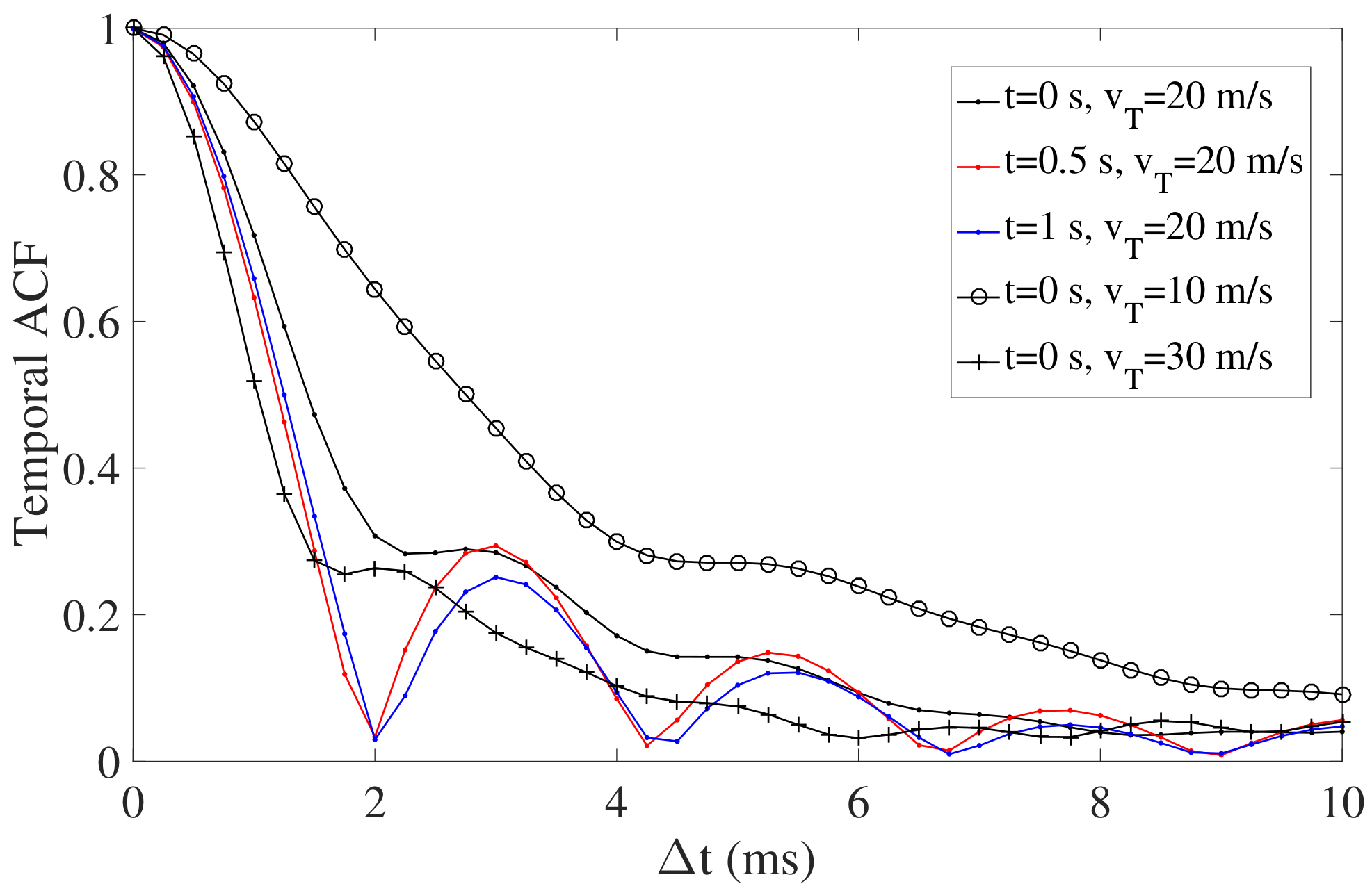
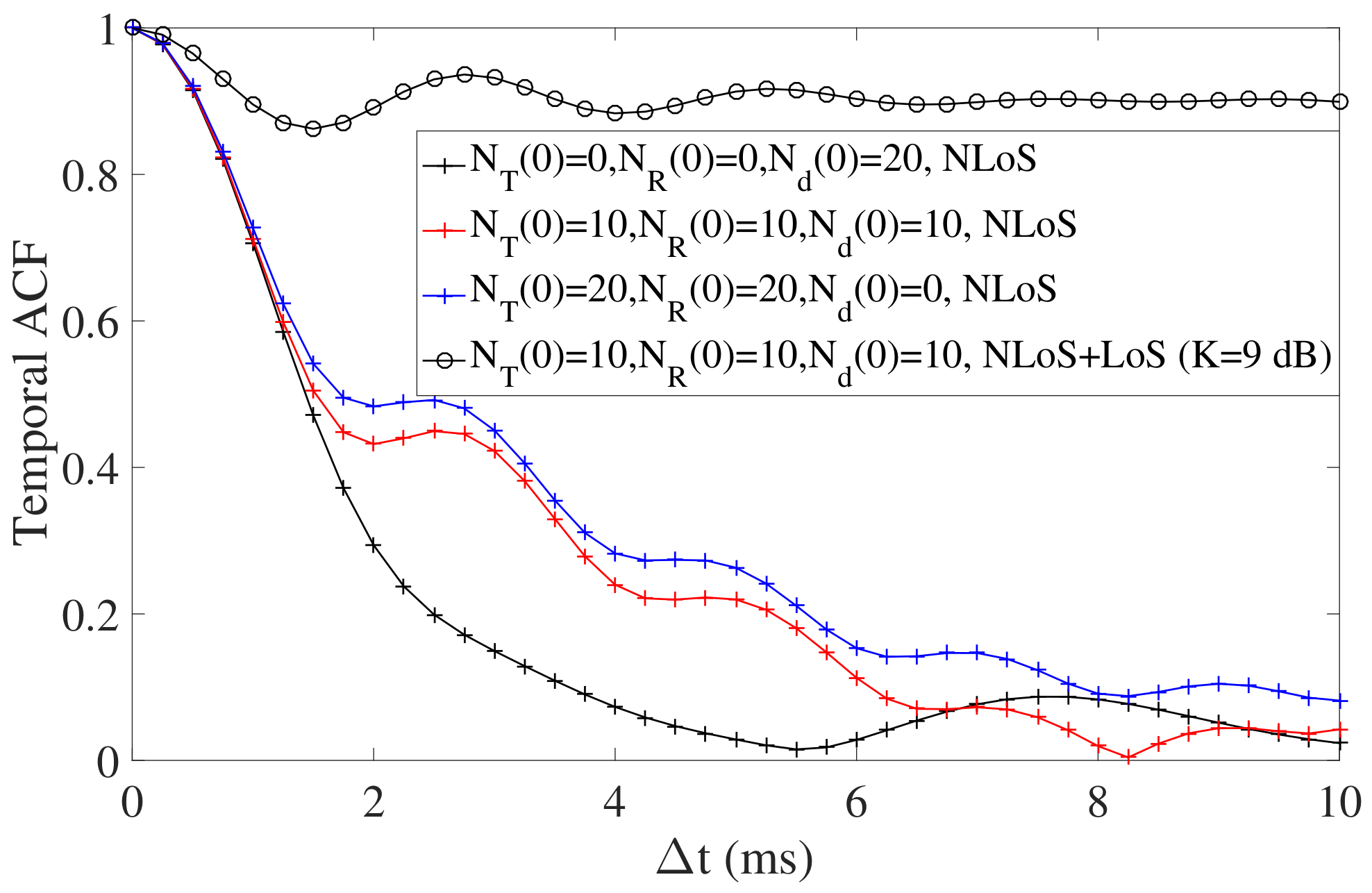
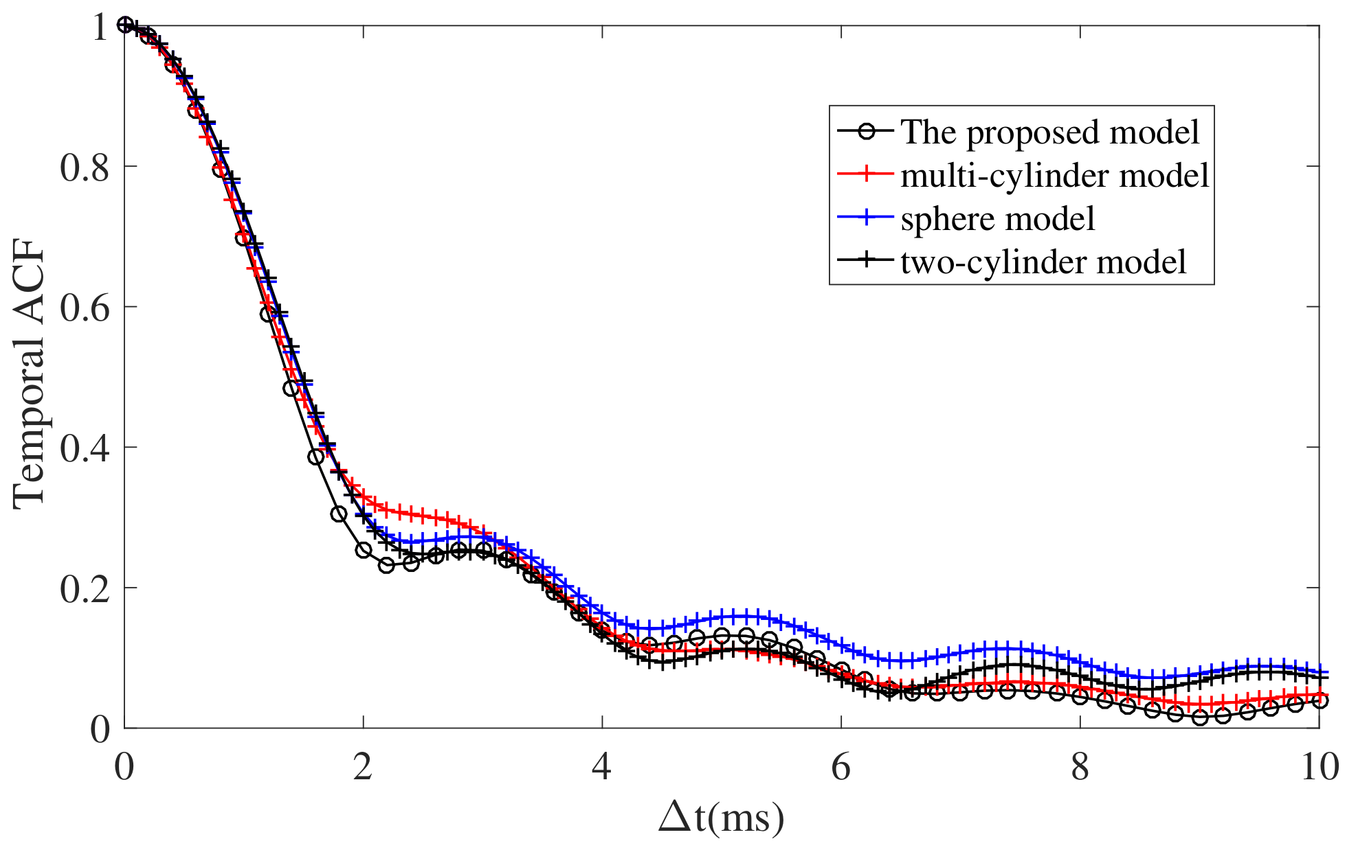
4.1. Space–Time Correlation Function

The ST-CF of the link between the ( p , q ) -th antenna and the ( p , q ) -th antenna as well as the link between the ( m , n ) -th antenna and the ( m , n ) -th antenna is computed by R ( p , q ) ( p , q ) , ( m , n ) ( m , n ) ( δ T , δ R , t , Δ t ) = E [ h ( p , q ) ( p , q ) ( t ) h ( m , n ) ( m , n ) ( t + Δ t ) ] E [ h ( p , q ) ( p , q ) ( t ) 2 ] E [ h ( m , n ) ( m , n ) ( t + Δ t ) 2 ] , in which ( · ) denotes the complex conjugate operation. Due to the introduction of the BD process, the survival probability of clusters becomes smaller as the update time progresses. And, the disappearance of clusters naturally leads to the disappearance of the corresponding channel characteristics. Thus, P sur i is a crucial part that contributes to the time correlation to describe the probability of clusters surviving in a time interval. Moreover, the ST-CF can be decomposed into the ST-CFs for different subcomponents, which is due to the mutual independence. The ST-CFs can be deduced as (20)–(23).
R ( p , q ) ( p , q ) , ( m , n ) ( m , n ) LoS ( δ T , δ R , t , Δ t ) = K K + 1 e j 2 π λ ( d ( p , q ) ( p , q ) ( t ) d ( m , n ) ( m , n ) ( t + Δ t ) ) e j 2 π t ( f d , LoS ( t ) f d , LoS ( t + Δ t ) ) j 2 π f d , LoS ( t + Δ t ) Δ t
R ( p , q ) ( p , q ) , ( m , n ) ( m , n ) SB , T ( δ T , δ R , t , Δ t ) = P sur T ( Δ t ) η 1 K + 1 n T = 1 N T ( t ) N T ( t + Δ t ) lim M n T P n T M n T E ( m n T = 1 M n T e j 2 π ( d n T , m n T SB , T t d n T , m n T SB , T ( t + Δ t ) ) / λ e j 2 π t ( f n T , m n T SB , T ( t ) f n T , m n T SB , T ( t + Δ t ) ) e j 2 π Δ t f n T , m n T SB , T ( t + Δ t ) ) = P sur T ( Δ t ) η 1 P n T K + 1 n T = 1 N T ( t ) N T ( t + Δ t ) π π π π e j 2 π ( d n T , m n T SB , T t d n T , m n T SB , T ( t + Δ t ) ) / λ e j 2 π t ( f n T , m n T SB , T ( t ) f n T , m n T SB , T ( t + Δ t ) ) e j 2 π Δ t f n T , m n T SB , T ( t + Δ t ) p ( ω n T , m n T T , γ n T , m n T T ) d ( ω n T , m n T T ) d ( γ n T , m n T T )
R ( p , q ) ( p , q ) , ( m , n ) ( m , n ) SB , R ( δ T , δ R , t , Δ t ) = P sur R ( Δ t ) η 2 P n R K + 1 n R = 1 N R ( t ) N R ( t + Δ t ) π π π π e j 2 π ( d n R , m n R SB , R t d n R , m n R SB , R ( t + Δ t ) ) / λ e j 2 π t ( f n R , m n R SB , R ( t ) f n R , m n R SB , R ( t + Δ t ) ) e j 2 π Δ t f n R , m n R SB , R ( t + Δ t ) p ( ω n R , m n R R , γ n R , m n R R ) d ( ω n R , m n R R ) d ( γ n R , m n R R )
R ( p , q ) ( p , q ) , ( m , n ) ( m , n ) MB ( δ T , δ R , t , Δ t ) = P sur MB ( Δ t ) η 3 P n MB K + 1 n d = 1 N d ( t ) N d ( t + Δ t ) π π π π π π π π e j 2 π ( d n d , m n d MB t d n d , m n d MB ( t + Δ t ) ) / λ e j 2 π t ( f n d , m n d MB ( t ) f n d , m n d MB ( t + Δ t ) ) e j 2 π Δ t f n d , m n d MB ( t + Δ t ) p ( ω n d , m n d MB , T , γ n d , m n d MB , T ) p ( ω n d , m n d MB , R , γ n d , m n d MB , R ) d ( ω n d , m n d MB , T ) d ( γ n d , m n d MB , T ) d ( ω n d , m n d MB , R ) d ( γ n d , m n d MB , R )

4.2. Angular Power Spectrum

The distribution of the power in the angular domain is reflected by the angular power spectrum. In the model, the angular power of the AoDs of clusters is derived, and it can be expressed as
λ ( t , μ ) = K K + 1 δ ( μ μ LoS ( t ) ) + η 1 K + 1 n T = 1 N T ( t ) P n T ( t ) δ ( μ μ n T ( t ) ) + η 2 K + 1 n R = 1 N R ( t ) P n R ( t ) δ ( μ μ n R ( t ) ) + η 3 K + 1 n d = 1 N d ( t ) P n d ( t ) δ ( μ μ n d ( t ) )
where μ n T / R / d denotes the AoD of the corresponding cluster.

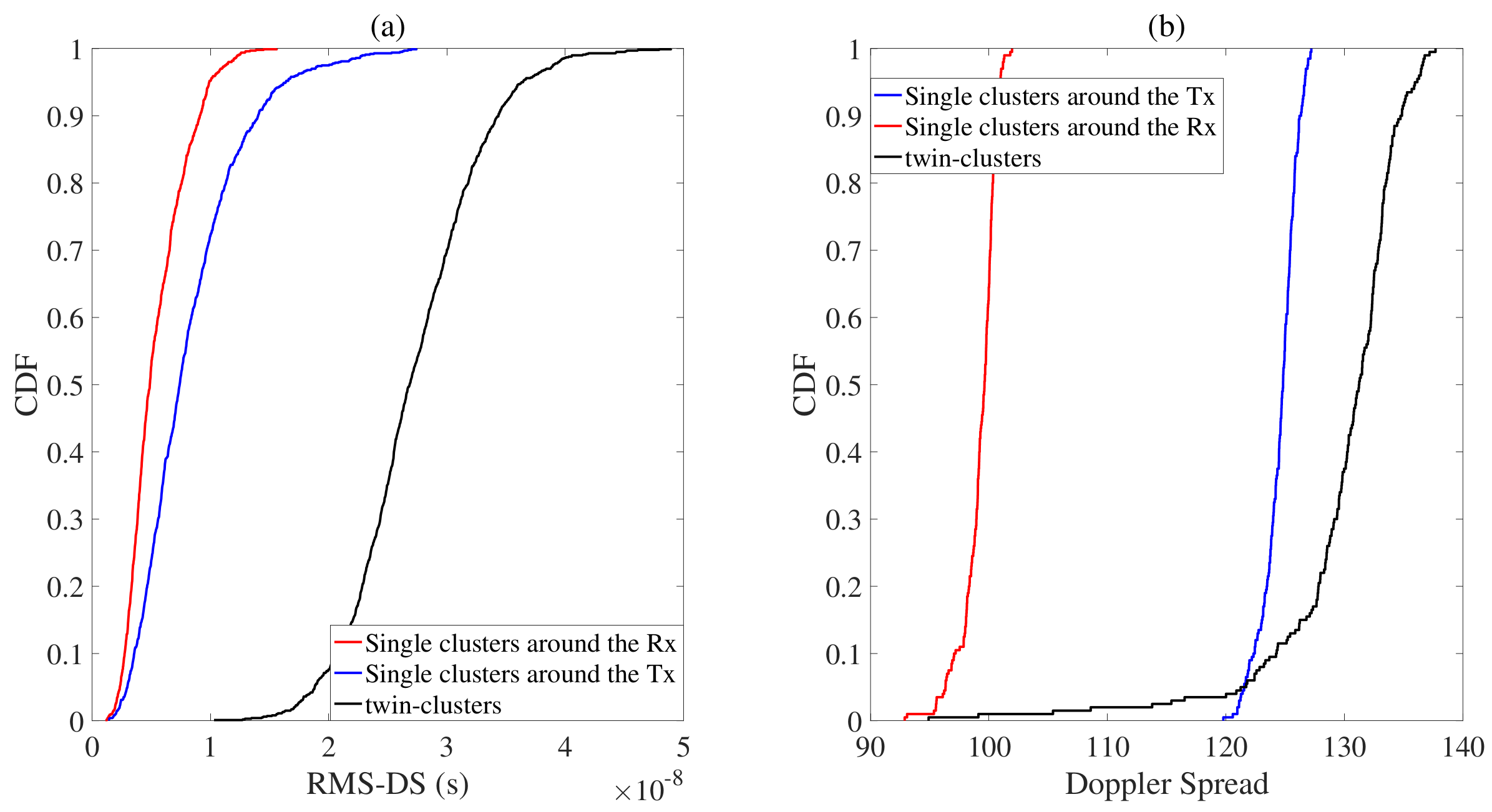
4.3. Root Mean Square Delay Spread

RMS-DS is one of the most important evaluation indices used to calculate the delay dispersion, and can be derived as
δ τ = l = 1 L P l ( t ) τ l 2 l = 1 L P l ( t ) τ l 2
where P l ( t ) and τ l are the normalized power and delay of the l-th cluster.

4.4. Doppler Spread

The instantaneous frequency can provide a power distribution in the frequency domain. The instantaneous mean Doppler shift and the instantaneous mean Doppler spread can be calculated by [52]
B f ( 1 ) = K K + 1 f d , LoS + i = 1 3 n = 1 N m n = 1 M n η i K + 1 P m n ( t ) f n , m n
B f ( 2 ) = ( K K + 1 f d , LoS 2 + i = 1 3 n = 1 N m n = 1 M n η i K + 1 P m n ( t ) f n , m n 2 ) ( B f ( 1 ) ) 2

4.5. Doppler PSD

Doppler PSD can be calculated by the Fourier transform of R ( p , q ) ( p , q ) , ( m , n ) ( m , n ) ( t , Δ t ) on Δ t , which can be written as
S ( p , q ) ( p , q ) , ( m , n ) ( m , n ) ( t , f D ) = R ( p , q ) ( p , q ) , ( m , n ) ( m , n ) ( t , Δ t ) e j 2 π f D Δ t d Δ t
where f D denotes the Doppler frequency.

4.6. Frequency Correlation Function

The time-variant channel transfer function H ( p , q ) ( p , q ) , ( m , n ) ( m , n ) ( t , f ) can be derived by the Fourier transform of the CIR. The FCF can be acquired by
R ( p , q ) ( p , q ) , ( m , n ) ( m , n ) ( t , Δ t , f , Δ f ) = E [ H ( p , q ) ( p , q ) ( t , f ) H ( m , n ) ( m , n ) ( t + Δ t , f + Δ f ) ] E [ H ( p , q ) ( p , q ) ( t , f ) 2 ] E [ H ( m , n ) ( m , n ) ( t + Δ t , f + Δ f ) 2 ]
The FCF can be derived as
R ( p , q ) ( p , q ) , ( m , n ) ( m , n ) ( t , Δ t , f , Δ f ) = K K + 1 e j 2 π f ( τ LoS ( Δ t + t ) τ LoS ( t ) ) + Δ f τ LoS ( Δ t + t ) + η 1 P n T K + 1 n T = 1 N T e j 2 π f ( τ n T ( Δ t + t ) τ n T ( t ) ) + Δ f τ n T ( Δ t + t ) + η 2 P n R K + 1 n R = 1 N R e j 2 π f ( τ n R ( Δ t + t ) τ n R ( t ) ) + Δ f τ n R ( Δ t + t ) + η 3 P n d K + 1 n d = 1 N d e j 2 π f ( τ n d ( Δ t + t ) τ n d ( t ) ) + Δ f τ n d ( Δ t + t )

5. Result and Analysis

In this section, the statistical properties are simulated and numerically analyzed. The channel parameters are set based on a reasonable assumption. Some of the parameters are given in Table 2, and other channel parameters are set as follows: f = 3.5 GHz, H T = 30 m, D = 300 m, v n T / R / MB U ( 0 , 10 ) m/s, θ n T / R / MB U ( 0 , π ) , v T = 20 m/s, v R = 20 m/s, ϕ T = π 4 , θ T = 0 , θ R = π , δ T = λ 2 , δ R = λ 2 , α T / R = π 4 , β T / R = π 4 , γ T / R = π 3 , r τ = 2.3 , δ τ = 10 6.63  [39], M T / R = 16 , N T / R = 16 . For low-altitude UAV communications, the environments around the UAV and the vehicle are similar, and thus the birth rate and death rate for clusters around the Tx and Rx are assumed to be equal, i.e., λ B = 10 , λ D = 2 , D c 1 / c 2 / c 3 = 50 , D a 1 / a 2 = 50 .
Time evolution and angular PSDs of single clusters and twin clusters are depicted in Figure 5. As mentioned before, twin clusters are randomly formed based on the simultaneous generation of new single clusters with probability P t w i n . When P t w i n = 0 , shown in (d–f), twin clusters do not have the conditions to produce. Therefore, twin clusters only contain two states, survival and death. In contrast, when P t w i n = 0.8 as shown in (a–c), new single clusters have a chance of merging into twin clusters, which may lead to a slower growth trend for the generation of single clusters. In this way, a suitable P t w i n can regulate the evolution speed as well as the trend of different types of clusters, and the relationship between different clusters is established. In addition, by combining with the transition region, the normalized angular PSDs are illustrated in (g–i). The birth-and-death properties are also represented in the angular domain. Moreover, the angular PSD of clusters around the Tx has more noticeable trajectory changes than clusters around the Rx due to faster angular variations resulting from closer distances. Additionally, on account of the largest delay caused by twin clusters, verified in (i), they contain the weakest power.
Figure 6 shows us the temporal ACFs for different airspeeds and at different time points. Obviously, the UAV with a high speed can generate a small temporal ACF, which can also be viewed in [40]. This is because a faster speed will cause more drastic changes in channel parameters in low-dynamic-channel environments and enhance the channel non-stationarity. In this case, a high speed will lead to a small temporal correlation. By comparing with the temporal ACFs at different time points, it can be seen that the temporal correlation changes over time, which verifies the channel non-stationarity in the time domain.
The temporal ACFs for different carrier frequencies and k R are depicted in Figure 7. Obviously, a large carrier frequency will lead to a small temporal correlation with a small coherence time, which is consistent with the conclusion in [53]. The phenomenon can be explained by the fact that a larger frequency has a smaller wavelength and leads to a more dispersive distribution of Doppler frequencies. In addition, as the concentration parameter k R increases, the temporal ACF shows a slower downtrend. k R controls the density of scatterers within clusters and scatterers are more concentrated around the average angles with the increase in k R , which results in a smaller angular spread.
Figure 8 depicts the temporal ACFs for a different number of single clusters and twin clusters. It is proved that twin clusters can accelerate the rate of the curve’s decline. As is mentioned, twin clusters can be considered as combinations of single clusters. Therefore, the AoDs and AoAs are mutually independent for twin clusters and the effect leads to a more flexible spatial distribution, which will be accompanied by channel parameters with a larger distribution range, including a more dispersive Doppler spread and delay spread. Another interesting observation is that the high power of the LoS component can enhance the temporal correlation markedly. This is because the LoS component contains dominant power and effectively alleviates the channel non-stationarity in the time domain.
The temporal ACF for a single—bounced component via C n T and C n R , respectively, is shown in Figure 9. The impact of the motion of the Tx, the Rx, and clusters on the temporal ACF is presented visually, and it is found that temporal ACFs dynamically change in the angular domain. This can verify the channel non-stationarity in the time domain once again. In addition, similar to [29], the temporal ACF is derived dependent on the distribution of scatterers and the area with dense scatterers results in a large temporal correlation. We also find that the horizontal movement of clusters will result in significant changes in azimuth angles. This is because the Tx, the Rx, and clusters move horizontally with different azimuth angles and thus azimuth angles contain more dramatic time-variant properties than elevation angles.
A comparison of the multi–cylinder model in [15], sphere model in [17], two–cylinder model in [19], and proposed channel model is shown in Figure 10. It can be seen that temporal ACFs share similar downward trends, which indicates the reasonability of the proposed model. In addition, we can perceive that although there are significant differences in the distribution of scatterers among models, a similar temporal correlation may be derived.
The space CCF R ( 1 , 1 ) ( 1 , 1 ) , ( 2 , 2 ) ( 2 , 2 ) ( δ T , t ) between the link from the ( 1 , 1 ) -th transmitting antenna to the ( 1 , 1 ) -th receiving antenna and the link from the ( 2 , 2 ) -th transmitting antenna to the ( 2 , 2 ) -th receiving antenna is explored in Figure 11. The space CCF has a faster descent speed with time, which proves the channel non-stationarity in the space domain. This is due to a greater angular spread resulting from the time-variant channel environment. Additionally, as k R increases, the space CCF shows a slower decline. This is because more dense scatterers distributed within a cluster will lead to a smaller angular spread and a smaller variance of distance differences.
Due to different spatial properties of the UPA compared to the ULA, the space CCF R ( 1 , 1 ) ( 1 , 1 ) , ( 1 , p ) ( 1 , 1 ) ( δ T ) and R ( 1 , 1 ) ( 1 , 1 ) , ( p , 1 ) ( 1 , 1 ) ( δ T ) are explored in Figure 12. It can be seen that antennas in the same row and in the same column show different space CCFs. This can be easily explained by the fact that the UPAs can be regarded as a combination of ULAs. Thus, antennas in the same row and in the same column can be regarded as linear antennas with different space angles. As we know, the spatial angle has an influence on the space CCF due to its impact on the angular spread [19]. In addition, when two antennas are further apart, the space correlation becomes smaller. It is also influenced by a larger angular spread. Moreover, the increase in | p p | will result in fewer clusters shared by both antennas, which is also a factor that changes the angular spread. Therefore, the spatial correlation does not decrease smoothly and a greater spatial correlation may emerge as the antenna index increases.
Figure 13 shows time-variant characteristics of the FCF. The simultaneous effect of the continuous and random occurrence and disappearance of clusters as well as the movement of surviving clusters, the UAV, and the vehicle results in severe frequency non-stationarity. Therefore, the FCF does not change smoothly over time and the BD properties contribute to strongly random changes in the FCF.
From Figure 14, we find that the carrier frequency and airspeed have a significant influence on the Doppler PSD. As the frequency increases, the Doppler PSD becomes wider with a larger Doppler spread. In addition, the peak moves to the right. This can be explained by the fact that a small wavelength will lead to a dispersive distribution of Doppler frequencies. Similarly, the increase in the airspeed can also effectively generate a wider Doppler PSD and maintain a similar curved shape. This indicates that the velocity of the UAV will change the values of Doppler frequencies; nevertheless, it will not have a significant impact on the distribution characteristics. Additionally, the movement of the peak is also a phenomenon resulting from the enlargement of Doppler frequencies.
Figure 15 compares the RMS—DSs (a) and Doppler spreads (b) of single clusters and twin clusters, respectively. It can be found that the RMS—DS of twin clusters is the largest, which indicates that twin clusters will generate a small correlation bandwidth. This is because multi–bounced components will result in greater delays. Another observation is that the RMS—DS of twin clusters has a dispersive distribution. This implies that the emergences and movements of twin clusters are more flexible than single clusters in 3D space. Futhermore, the flexible spatial characteristics of twin clusters can also lead to a dispersive distribution of Doppler frequencies. When the AoAs or AoDs are determined by the locations of single clusters, the AoDs or AoAs of single clusters are fixed values. By contrast, the AoAs and AoDs of twin clusters are separately determined by two different single clusters randomly generated in 3D space. As a result, twin clusters have a wider angular distribution, which also enlarges the distribution range of Doppler frequencies.

6. Conclusions

A novel cluster-based low-altitude U2V non-stationary channel model with UPAs is proposed in the paper. The proposed channel model takes into account both single clusters and twin clusters. In order to model the U2V non-stationarity, an improved cluster evolution algorithm is developed to integrate continuous time evolution and array evolution. In the time evolution, new single clusters evolve based on the BD property and the formation of twin clusters relies on the simultaneous generation of new single clusters around the Tx and Rx with a correlation probability P t w i n . P t w i n is proven to effectively regulate the evolutionary trends of different types of clusters. In addition, the developed array evolution algorithm for new clusters and survival clusters applied to UPAs is proved to satisfy the coherence and regionality of antenna sets. At the same time, time-variant channel parameters and channel statistical properties are derived. The simulated results prove that the proposed model can effectively capture the non-stationarity in the time, space, and frequency domain. The numerical analysis validates that twin clusters flexibly generated in 3D space contain low power and that the flexibility leads to a large distribution range of the RMS-DS and Doppler spread. Moreover, the wide distribution range of twin clusters also contributes to the fast decline in the temporal ACF as well as a large RMS-DS. We also find that the increase in the airspeed leads to a small temporal correlation and a large Doppler PSD. As scatterers become more concentrated, the space CCF and temporal ACF get large. Additionally, a large Doppler spread and temporal ACF can be observed with a large carrier frequency. The reasonability of the proposed model is also verified through comparison with other GBSMs. Undoubtedly, the speed of the UAV, the selection of carrier frequency, and changes in the scattering environment can have a perceptible effect on the channel characteristics. The characteristic difference between SB and MB components is also simulated and evaluated by single and twin clusters. These conclusions are helpful in the performance evaluation and optimization of UAV communication systems.

Author Contributions

Conceptualization, Z.S. and C.L.; methodology, Z.S.; validation, Z.S., W.C. and C.L.; formal analysis, Z.S. and W.C.; investigation, C.L.; writing—original draft preparation, Z.S.; writing—review and editing, Z.S. and W.C.; supervision, W.C. and C.L. All authors have read and agreed to the published version of the manuscript.

Funding

This work was supported by National Natural Science Foundation of China (No. 52102399) and Key Research and Development Program of Hubei Province (2023BAB052).

Data Availability Statement

No new data were created.

Conflicts of Interest

The authors declare no conflict of interest.

References

  1. Zhang, Z.; Xiao, Y.; Ma, Z.; Xiao, M.; Ding, Z.; Lei, X.; Karagiannidis, G.K.; Fan, P. 6G wireless networks: Vision, requirements, architecture, and key technologies. IEEE Veh. Technol. Mag. 2019, 14, 28–41. [Google Scholar] [CrossRef]
  2. Liu, J.; Shi, Y.; Fadlullah, Z.M.; Kato, N. Space-air-ground integrated network: A survey. IEEE Commun. Surv. Tutor. 2018, 20, 2714–2741. [Google Scholar] [CrossRef]
  3. Hayat, S.; Yanmaz, E.; Muzaffar, R. Survey on unmanned aerial vehicle networks for civil applications: A communications viewpoint. IEEE Commun. Surv. Tutor. 2016, 18, 2624–2661. [Google Scholar] [CrossRef]
  4. Wang, C.X.; Huang, J.; Wang, H.; Gao, X.; You, X.; Hao, Y. 6G oriented wireless communication channel characteristics analysis and modeling. arXiv 2020, arXiv:2007.13958. [Google Scholar]
  5. Khuwaja, A.A.; Chen, Y.; Zhao, N.; Alouini, M.S.; Dobbins, P. A survey of channel modeling for UAV communications. IEEE Commun. Surv. Tutor. 2018, 20, 2804–2821. [Google Scholar] [CrossRef]
  6. Cui, Z.; Briso-Rodríguez, C.; Guan, K.; Calvo-Ramírez, C.; Ai, B.; Zhong, Z. Measurement-based modeling and analysis of UAV air-ground channels at 1 and 4 GHz. IEEE Antennas Wirel. Propag. Lett. 2019, 18, 1804–1808. [Google Scholar] [CrossRef]
  7. Khawaja, W.; Guvenc, I.; Matolak, D.W.; Fiebig, U.C.; Schneckenburger, N. A survey of air-to-ground propagation channel modeling for unmanned aerial vehicles. IEEE Commun. Surv. Tutor. 2019, 21, 2361–2391. [Google Scholar] [CrossRef]
  8. Wang, K.; Zhang, R.; Wu, L.; Zhong, Z.; He, L.; Liu, J.; Pang, X. Path loss measurement and modeling for low-altitude UAV access channels. In Proceedings of the 2017 IEEE 86th Vehicular Technology Conference (VTC-Fall), Toronto, ON, Canada, 24–27 September 2017; pp. 1–5. [Google Scholar]
  9. Cai, X.; Gonzalez-Plaza, A.; Alonso, D.; Zhang, L.; Rodríguez, C.B.; Yuste, A.P.; Yin, X. Low altitude UAV propagation channel modelling. In Proceedings of the 2017 11th European Conference on Antennas and Propagation (EUCAP), Paris, France, 19–24 March 2017; pp. 1443–1447. [Google Scholar]
  10. Matolak, D.W.; Sun, R. Air-ground channels for UAS: Summary of measurements and models for L-and C-bands. In Proceedings of the 2016 Integrated Communications Navigation and Surveillance (ICNS), Herndon, VA, USA, 19–21 April 2016; pp. 8B2-1–8B2-11. [Google Scholar]
  11. Willink, T.J.; Squires, C.C.; Colman, G.W.K.; Muccio, M.T. Measurement and characterization of low-altitude air-to-ground MIMO channels. IEEE Trans. Veh. Technol. 2015, 65, 2637–2648. [Google Scholar] [CrossRef]
  12. Matolak, D.W.; Jamal, H.; Sun, R. Spatial and frequency correlations in two-ray air-ground SIMO channels. In Proceedings of the 2017 IEEE International Conference on Communications (ICC), Paris, France, 21–25 May 2017; pp. 1–6. [Google Scholar]
  13. Gao, X.; Chen, Z.; Hu, Y. Analysis of unmanned aerial vehicle MIMO channel capacity based on aircraft attitude. WSEAS Trans. Inform. Sci. Appl. 2013, 10, 58–67. [Google Scholar]
  14. Greenberg, E.; Levy, P. Channel characteristics of UAV to ground links over multipath urban environments. In Proceedings of the 2017 IEEE International Conference on Microwaves, Antennas, Communications and Electronic Systems (COMCAS), Tel-Aviv, Israel, 13–15 November 2017; pp. 1–4. [Google Scholar]
  15. Bian, J.; Wang, C.X.; Liu, Y.; Tian, J.; Qiao, J.; Zheng, X. 3D non-stationary wideband UAV-to-ground MIMO channel models based on aeronautic random mobility model. IEEE Trans. Veh. Technol. 2021, 70, 11154–11168. [Google Scholar] [CrossRef]
  16. Ma, Z.; Ai, B.; He, R.; Wang, G.; Niu, Y.; Yang, M.; Zhong, Z. Impact of UAV rotation on MIMO channel characterization for air-to-ground communication systems. IEEE Trans. Veh. Technol. 2020, 69, 12418–12431. [Google Scholar] [CrossRef]
  17. Jia, R.; Li, Y.; Cheng, X.; Ai, B. 3D geometry-based UAV-MIMO channel modeling and simulation. China Commun. 2018, 15, 64–74. [Google Scholar]
  18. Jin, K.; Cheng, X.; Ge, X.; Yin, X. Three dimensional modeling and space-time correlation for UAV channels. In Proceedings of the 2017 IEEE 85th Vehicular Technology Conference (VTC Spring), Sydney, NSW, Australia, 4–7 June 2017; pp. 1–5. [Google Scholar]
  19. Cheng, X.; Li, Y.; Wang, C.X.; Yin, X.; Matolak, D.W. A 3-D geometry-based stochastic model for unmanned aerial vehicle MIMO Ricean fading channels. IEEE Internet Things J. 2020, 7, 8674–8687. [Google Scholar] [CrossRef]
  20. Zhang, X.; Cheng, X. Second order statistics of simulation models for UAV-MIMO Ricean fading channels. In Proceedings of the ICC 2019—2019 IEEE International Conference on Communications (ICC), Shanghai, China, 20–24 May 2019; pp. 1–6. [Google Scholar]
  21. Mao, J.; Wei, Z.; Liu, K.; Cheng, Z.; Cheng, B.; Li, H. A 3D air-to-ground channel model based on a street scenario. In Proceedings of the 2020 IEEE 6th International Conference on Computer and Communications (ICCC), Chengdu, China, 11–14 December 2020; pp. 1356–1362. [Google Scholar]
  22. Jiang, H.; Zhang, Z.; Gui, G. Three-dimensional non-stationary wideband geometry-based UAV channel model for A2G communication environments. IEEE Access 2019, 7, 26116–26122. [Google Scholar] [CrossRef]
  23. Chang, H.; Bian, J.; Wang, C.X.; Bai, Z.; Zhou, W. A 3D non-stationary wideband GBSM for low-altitude UAV-to-ground V2V MIMO channels. IEEE Access 2019, 7, 70719–70732. [Google Scholar] [CrossRef]
  24. Lian, Z.; Su, Y.; Wang, Y.; Jiang, L.; Zhang, Z.; Xie, Z.; Li, S. A nonstationary 3-D wideband channel model for low-altitude UAV-MIMO communication systems. IEEE Internet Things J. 2021, 9, 5290–5303. [Google Scholar] [CrossRef]
  25. Zhang, Y.; Zhou, Y.; Ji, Z.; Lin, K.; He, Z. A three-dimensional geometry-based stochastic model for air-to-air UAV channels. In Proceedings of the 2020 IEEE 92nd Vehicular Technology Conference (VTC2020-Fall), Victoria, BC, Canada, 18 November–16 December 2020; pp. 1–5. [Google Scholar]
  26. Zeng, L.; Cheng, X.; Wang, C.X.; Yin, X. A 3D geometry-based stochastic channel model for UAV-MIMO channels. In Proceedings of the 2017 IEEE Wireless Communications and Networking Conference (WCNC), San Francisco, CA, USA, 19–22 March 2017; pp. 1–5. [Google Scholar]
  27. Ma, Z.; Ai, B.; He, R.; Zhong, Z.; Yang, M.; Wang, J.; Li, J. Three-dimensional modeling of millimeter-wave MIMO channels for UAV-based communications. In Proceedings of the GLOBECOM 2020–2020 IEEE Global Communications Conference, Taipei, Taiwan, 7–11 December 2020; pp. 1–6. [Google Scholar]
  28. Xu, J.; Cheng, X.; Bai, L. A 3-D space-time-frequency non-stationary model for low-altitude UAV mmWave and massive MIMO aerial fading channels. IEEE Trans. Antennas Propag. 2022, 70, 10936–10950. [Google Scholar] [CrossRef]
  29. Ji, W.; Zhang, Z.Z.; Hu, H. A Novel 3D Non-stationary Single-twin cluster Model for Mobile-mobile MIMO Channels. In Proceedings of the 2020 IEEE/CIC International Conference on Communications in China (ICCC), Chongqing, China, 9–11 August 2020; pp. 693–698. [Google Scholar]
  30. He, R.; Ai, B.; Stuber, G.L.; Wang, G.; Zhong, Z. A cluster based geometrical model for millimeter wave mobile-to-mobile channels. In Proceedings of the 2017 IEEE/CIC International Conference on Communications in China (ICCC), Qingdao, China, 22–24 October 2017; pp. 1–6. [Google Scholar]
  31. Xie, X.; Zhang, Z.; Jiang, H.; Dang, J.; Wu, L. Cluster-based geometrical dynamic stochastic model for MIMO scattering channels. In Proceedings of the 2017 9th international conference on wireless communications and signal processing (WCSP), Nanjing, China, 11–13 October 2017; pp. 1–5. [Google Scholar]
  32. Li, Y.; He, R.; Lin, S.; Guan, K.; He, D.; Wang, Q.; Zhong, Z. Cluster-based nonstationary channel modeling for vehicle-to-vehicle communications. IEEE Antennas Wirel. Propag. Lett. 2016, 16, 1419–1422. [Google Scholar] [CrossRef]
  33. Liu, Y.; Wang, C.X.; Chang, H.; He, Y.; Bian, J. A novel non-stationary 6G UAV channel model for maritime communications. IEEE J. Sel. Areas Commun. 2021, 39, 2992–3005. [Google Scholar] [CrossRef]
  34. Liu, Y.; Wang, C.X.; Huang, J.; Sun, J.; Zhang, W. Novel 3-D nonstationary mmWave massive MIMO channel models for 5G high-speed train wireless communications. IEEE Trans. Veh. Technol. 2018, 68, 2077–2086. [Google Scholar] [CrossRef]
  35. Chang, H.; Wang, C.X.; Liu, Y.; Huang, J.; Sun, J.; Zhang, W.; Gao, X. A novel nonstationary 6G UAV-to-ground wireless channel model with 3-D arbitrary trajectory changes. IEEE Internet Things J. 2020, 8, 9865–9877. [Google Scholar] [CrossRef]
  36. Bai, L.; Huang, Z.; Zhang, X.; Cheng, X. A non-stationary 3D model for 6G massive MIMO mmWave UAV channels. IEEE Trans. Wirel. Commun. 2021, 21, 4325–4339. [Google Scholar] [CrossRef]
  37. Wu, S.; Wang, C.X.; Alwakeel, M.M.; You, X. A general 3-D non-stationary 5G wireless channel model. IEEE Trans. Commun. 2017, 66, 3065–3078. [Google Scholar] [CrossRef]
  38. Wu, S.; Wang, C.X.; Haas, H.; Alwakeel, M.M.; Ai, B. A non-stationary wideband channel model for massive MIMO communication systems. IEEE Trans. Wirel. Commun. 2014, 14, 1434–1446. [Google Scholar] [CrossRef]
  39. Wu, S.; Wang, C.X.; Alwakeel, M.M.; He, Y. A non-stationary 3-D wideband twin-cluster model for 5G massive MIMO channels. IEEE J. Sel. Areas Commun. 2014, 32, 1207–1218. [Google Scholar] [CrossRef]
  40. Bai, L.; Huang, Z.; Li, Y.; He, Y. A 3D cluster-based channel model for 5G and beyond vehicle-to-vehicle massive MIMO channels. IEEE Trans. Veh. Technol. 2021, 70, 8401–8414. [Google Scholar] [CrossRef]
  41. Bai, L.; Huang, Z.; Cui, L.; Feng, T.; Cheng, X. A mixed-bouncing based non-stationary model for 6G massive MIMO mmWave UAV channels. IEEE Trans. Commun. 2022, 70, 7055–7069. [Google Scholar] [CrossRef]
  42. Huang, Z.; Cheng, X. A general 3D space-time-frequency non-stationary model for 6G channels. IEEE Trans. Wirel. Commun. 2020, 20, 535–548. [Google Scholar] [CrossRef]
  43. Huang, Z.; Cheng, X.; Yin, X. A general 3D non-stationary 6G channel model with time-space consistency. IEEE Trans. Commun. 2022, 70, 3436–3450. [Google Scholar] [CrossRef]
  44. Liu, L.; Oestges, C.; Poutanen, J.; Haneda, K.; Vainikainen, P.; Quitin, F.; De Doncker, P. The COST 2100 MIMO channel model. IEEE Wirel. Commun. 2012, 19, 92–99. [Google Scholar] [CrossRef]
  45. Bian, J.; Wang, C.X.; Huang, J.; Liu, Y.; Sun, J.; Zhang, M.; Aggoune, E.H.M. A 3D wideband non-stationary multi-mobility model for vehicle-to-vehicle MIMO channels. IEEE Access 2019, 7, 32562–32577. [Google Scholar] [CrossRef]
  46. Bai, L.; Huang, Z.; Du, H.; Cheng, X. A 3-D Nonstationary Wideband V2V GBSM With UPAs for Massive MIMO Wireless Communication Systems. IEEE Internet Things J. 2021, 8, 17622–17638. [Google Scholar] [CrossRef]
  47. Ma, N.; Chen, J.; Zhang, P.; Yang, X. Novel 3-D irregular-shaped model for massive MIMO V2V channels in street scattering environments. IEEE Wirel. Commun. Lett. 2020, 9, 1437–1441. [Google Scholar] [CrossRef]
  48. Jiang, H.; Ying, W.; Zhou, J.; Shao, G. A 3D wideband two-cluster channel model for massive MIMO vehicle-to-vehicle communications in semi-ellipsoid environments. IEEE Access 2020, 8, 23594–23600. [Google Scholar] [CrossRef]
  49. Chang, H.; Wang, C.X.; Liu, Y.; Huang, J.; Sun, J.; Zhang, W.; Aggoune, E.H.M. A General 3-D Nonstationary GBSM for Underground Vehicular Channels. IEEE Trans. Antennas Propag. 2022, 71, 1804–1819. [Google Scholar] [CrossRef]
  50. Zhu, Q.; Jiang, K.; Chen, X.; Zhong, W.; Yang, Y. A novel 3D non-stationary UAV-MIMO channel model and its statistical properties. China Commun. 2018, 15, 147–158. [Google Scholar]
  51. Bian, J.; Sun, J.; Wang, C.X.; Feng, R.; Huang, J.; Yang, Y.; Zhang, M. A WINNER+ based 3-D non-stationary wideband MIMO channel model. IEEE Trans. Wirel. Commun. 2017, 17, 1755–1767. [Google Scholar] [CrossRef]
  52. Ge, C.; Zhang, R.; Jiang, Y.; Li, B.; He, Y. A 3-D dynamic non-WSS cluster geometrical-based stochastic model for UAV MIMO channels. IEEE Trans. Veh. Technol. 2022, 71, 6884–6899. [Google Scholar] [CrossRef]
  53. Ma, Z.; Ai, B.; He, R.; Zhong, Z.; Yang, M. A non-stationary geometry-based MIMO channel model for millimeter-wave UAV networks. IEEE J. Sel. Areas Commun. 2021, 39, 2960–2974. [Google Scholar] [CrossRef]
Figure 1. A 3D non-stationary channel model for low-altitude UAV-to-vehicle communications.
Drones 07 00640 g001
Figure 2. Flowchart of cluster evolution.
Drones 07 00640 g002
Figure 3. Power variation of time-varying clusters.
Drones 07 00640 g003
Figure 4. Array evolution of the transmitting UPA.
Drones 07 00640 g004
Figure 5. Time evolution with P t w i n = 0.8 (ac): clusters around the Tx, clusters around the Rx, and twin clusters. Time evolution with P t w i n = 0 (df): clusters around the Tx, clusters around the Rx, and twin clusters. normalized angular PSD (gi): clusters around the Tx, clusters around the Rx, and twin clusters.
Drones 07 00640 g005
Figure 6. The temporal ACFs for different velocities of the UAV and at different time points.
Drones 07 00640 g006
Figure 7. The temporal ACFs for different frequencies and k R .
Drones 07 00640 g007
Figure 8. The temporal ACFs for different number of single clusters and twin clusters.
Drones 07 00640 g008
Figure 9. The normalized temporal ACF in the angular domain.
Drones 07 00640 g009
Figure 10. The normalized temporal ACF of the proposed model, multi−cylinder model in [15], sphere model in [17], and two−cylinder model in [19]. ( f = 3.5 GHz, H T = 30 m, D = 300 m, v T = 20 m/s, v R = 20 m/s, ϕ T = π 4 , θ T = 0 , θ R = π , δ T = λ 2 , δ R = λ 2 , α T / R = π 4 , β T / R = π 4 , γ T / R = π 3 ).
Drones 07 00640 g010
Figure 11. The space CCF in terms of transmitting antenna spacing with different k R and at different time points.
Drones 07 00640 g011
Figure 12. The space CCF in terms of transmitting UPAs.
Drones 07 00640 g012
Figure 13. The FCF with time.
Drones 07 00640 g013
Figure 14. Doppler PSDs for different frequencies and with different airspeeds.
Drones 07 00640 g014
Figure 15. (a) RMS—DSs for different types of clusters. (b) Doppler spread for different categories of clusters.
Drones 07 00640 g015
Table 1. A comparison of the latest GBSMs.
ModelsChannelsMethods for Describing Channel ModelsMethods for Capturing Non-StationarityAntenna Type
Model in [17,18,19,20,25,26]UAV communicationsRegular geometry/uniform linear arrays (ULAs)
Model in [15,21,22]UAV communicationsRegular geometryTime-variant channel parametersULAs
Model in [23,24,27]UAV communicationsRegular geometryTime-variant channel parameters and time evolutionULAs
Model in [48]Vehicle communicationsRegular geometryTime-variant channel parameters and array evolutionULAs
Model in [32]Vehicle communicationsSingle clusters and twin clustersTime-variant channel parameters and time evolutionULAs
Model in [31,45]Vehicle communicationsSingle clustersTime-variant channel parametersULAs
Model in [35,36]UAV communicationsTwin clustersTime-variant channel parameters, time and array evolutionULAs
Model in [46]Vehicle communicationsRegular geometryTime-variant channel parameters, time and array evolutionuniform planar arrays (UPAs)
Model in [41]UAV communicationsSingle clusters and twin clustersTime-variant channel parameters, time and array evolutionULAs
The proposed modelUAV communicationsSingle clusters and twin clustersTime-variant channel parameters, time and array evolutionUPAs
Table 2. Distribution of relevant channel parameters.
ParameterDistributionMeanDerivation
ω n T T , ω n R R wrapped Gaussian 60 ° , 180 ° 20 ° , 30 °
γ n T T , γ n R R wrapped Gaussian 45 ° , 45 ° 30 ° , 30 °
D n T , D n R exponential 1 30 , 1 30 1 900 , 1 900
Disclaimer/Publisher’s Note: The statements, opinions and data contained in all publications are solely those of the individual author(s) and contributor(s) and not of MDPI and/or the editor(s). MDPI and/or the editor(s) disclaim responsibility for any injury to people or property resulting from any ideas, methods, instructions or products referred to in the content.

