Article

Dynamic Robust Spectrum Sensing Based on Goodness-of-Fit Test Using Bilateral Hypotheses

1
School of Medical Information Engineering, Guangzhou University of Chinese Medicine, Guangzhou 510006, China
2
Institut d’Electronique et Télécommunications de Rennes (IETR), Université de Nantes, UMR CNRS 6164, Rue Christian Pauc BP 50609, 44306 Nantes, France
3
School of Integrated Circuits, Guangdong University of Technology, Guangzhou 510006, China
*
Author to whom correspondence should be addressed.
Drones 2023, 7(1), 18; https://doi.org/10.3390/drones7010018
Submission received: 28 November 2022 / Revised: 18 December 2022 / Accepted: 23 December 2022 / Published: 27 December 2022
(This article belongs to the Special Issue UAV-Assisted Intelligent Vehicular Networks)

Abstract

:
Dynamic spectrum detection has attracted increasing interest in drone or drone controller detection problems. Spectrum sensing as a promising solution allows us to provide a dynamic spectrum map within the target frequency band by estimating the occupied sub-bands in a specific period. In this paper, a robust Student’s t-distribution model is built to tackle the scenario with a small number of observed samples. Then, relying on the characteristics of the statistical model, we propose an appropriate goodness-of-fit (GoF) test statistic regarding a small number of samples. Moreover, to obtain a reliable sensing, bilateral hypotheses of the test statistic are both used to make a decision. Numerical simulations show the superiority of the proposed method compared with other schemes, including the unilateral hypothesis-based GoF testing and the conventional energy detection, in a small number of sample cases.

1. Introduction

Nowadays, due to the rapid development of the wireless communication, the number of civil unmanned aerial vehicles (UAVs) has increased significantly in recent years, which could cause many problems for city administration [1]. Reliable detection of UAVs or their controllers is a prerequisite for further administration [2,3,4]. Cognitive radio (CR) [5], which enables dynamic detection of surrounding signal spectrum, becomes a promising solution for frequency detection. More specifically, the whole spectrum can be divided into sub-bands and different signal occupancies can be estimated [6,7,8]. It has been widely applied to drone networks in order to create promising infrastructures of cognitive drone networks, in which multiple resource-constrained sensor nodes are equipped with cognitive ability [9,10,11,12]. As the fundamental prerequisite for CR, namely spectrum sensing (SS) [13,14], reliable and quick detection of signal existence is the key for further strategy and decision.
To dynamically estimate the existing spectrum, many algorithms have been developed, including cyclostationary feature, matched filter, waveform-based detection [15,16,17], etc. However, these algorithms need to acquire prior knowledge of primary user (PU), which is difficult in practice, i.e., illegal quad-rotor drone intrusion. Therefore, blind detection techniques that do not need prior knowledge about PU are developed, for instance, the energy detection (ED) scheme [18,19,20] and the eigenvalue-based estimation [21,22,23]. ED is one commonly adopted method due to its simplicity for implementation, but the noise uncertainty in practice significantly degrades its detection performance. Thus, the eigenvalue-based blind detection is proposed to settle the disadvantage of ED by analyzing the covariance matrix. The corresponding eigenvalues are utilized to increase the robustness against noise uncertainty. Unfortunately, it needs a large number of samples to obtain a good performance, and has relatively high complexity.
Some GoF test-based strategies have been proposed to achieve better estimation performance given a small number of available samples [24,25,26,27,28,29,30]. In [31], the Anderson–Darling (AD) test is exploited to achieve reliable detection under a small number of samples. On the basis of this, the authors in [32] make use of a Student’s t-distribution test for fully blind detection with noise uncertainty. In [33], the Kolmogorov–Smirnov (KS) test, a non-parametric GoF method, is used to perform a fast and reliable spectrum sensing, which is also robust to non-Gaussian noise and channel uncertainty. In [34], the authors utilize a powerful GoF test to achieve non-parametric sensing for Middleton noise scenario. In [35], the characteristic of non-symmetrical differences is exploited to construct the unilateral right-tail AD test. In [36], the ratio between maximum eigenvalue relative to the trace is exploited to achieve blind detection. However, only one side of the binary hypothesis information is used in all of the above works. That is to say, only the null hypothesis is considered. Therefore, the reliability of the decision may be improved by using the bilateral hypotheses.
To address the above problems, an enhanced detection method based on the GoF test using bilateral hypotheses for a small number of samples in cognitive drone network is proposed in this work. One of the main objectives is to obtain a short signal processing and a real-time decision. Considering the case that there is only a single-radio module at SU, the sampling period of the observation sensors is expected to be as short as possible. Moreover, we consider a special information environment where there is only few steady state receptions available. First of all, we propose to utilize the Student’s t-distribution in order to address a small number of sample problems, which are collected by the low power sensor nodes (SU) in the cognitive drone network. In fact, the performance of ED using Gaussian approximation becomes good only when sufficiently large sample size is available [37]. It has been shown that the Student’s t-test is the optimal test in spectrum sensing given a small number of samples [38,39]. Then, taking into account the limitations of the traditional GoF test (e.g., AD test and KS test) under a small number of samples, the powerful GoF test [40,41,42,43,44] is introduced to precisely evaluate the distance between common cumulative distribution and the empirical distribution of observation. As in the proposed method in [45], the statistic based on the likelihood ratio is used, which is substantially more powerful than the traditional statistic. The main contribution stands in the proposition of the powerful GoF test to accommodate the small samples situation. Finally, two new statistics based on bilateral hypotheses are calculated based on the statistical characteristic of Student’s t-distribution, and a high reliability sensing decision is obtained based on bilateral hypotheses.
The rest of the paper is organized as follows. The traditional unilateral hypothesis-based GoF test is introduced in Section 2. The proposed scheme is illustrated in Section 3, where the Student’s t-distribution-based statistical model is provided. A powerful goodness-of-fit test statistic Z c is introduced for computing the distance between the common cumulative distribution of the observations and the empirical distribution, and the bilateral hypotheses information is utilized for high reliability decision. Numerical simulations are discussed in Section 4 and the conclusions are provided in Section 5.

2. Traditional GoF Test Based on Unilateral Hypothesis

The traditional sensing scheme on the basis of GoF test using unilateral hypothesis is presented in this section. Spectrum sensing aims to detect the existence of PU signal in a specific frequency band for a given set of observed samples. This can be expressed as a traditional GoF test problem, which can be written as:
H 0 : F n ( x ) = F 0 ( x ) H 1 : F n ( x ) F 0 ( x )
where H 0 is the null hypothesis and H 1 is the alternative hypothesis. F 0 ( x ) denotes the cumulative distribution function (CDF) of noise distribution of H 0 hypothesis, while F n ( x ) represents the CDF of collected samples, which can be calculated by using the empirical CDF
F n ( x ) = | i : x i x , 1 i n | / n
where | S | represents the cardinality of a given set S, and n denotes the number of samples utilized for acquiring the statistical distribution.
In other words, the detection problem is turned to a problem of testing the null hypothesis against the alternative hypothesis. Assuming that Z is a statistic for testing H 0 against H 1 , which is defined as [46]
Z = Z x d w ( x ) .
Here, w ( x ) represents some weight function and large values of Z and reject the null hypothesis H 0 . The power of Z depends on Z x and w ( x ) , and the natural candidate for Z x is generally considered as the Pearson χ 2 test statistic defined as follows [46]:
P x 2 = n ( F n ( x ) F 0 ( x ) ) 2 F 0 ( x ) ( 1 F 0 ( x ) ) .
For a traditional GoF test, Z x in Equation (3) is firstly replaced by P x 2 . Then, various traditional GoF tests have been proposed to evaluate the distance between F 0 ( x ) and F n ( x ) , and how to choose different weight functions. For instance, the AD test, Kolmogorov–Smirnov (KS) test, and Cramér-von Mises (CM) test [47,48]. They belong to the one-side hypothesis test for H 0 . A one-side hypothesis is utilized for determining whether the collected samples meet the distribution with CDF F 0 ( x ) or not. These GoF tests are illustrated as follows.
(A)
KS test: To evaluate the relative distance, the empirical CDF of collected samples and the reference CDF are considered in KS test and w ( x ) = n 1 F 0 ( x ) ( 1 F 0 ( x ) ) is chosen. Then, the GoF test statistic can be obtained using the largest absolute distance between the two CDFs, which can be written as
D 2 = { sup | F n ( x ) F 0 ( x ) | } 2 .
Here, sup { · } represents the supremum function denoting the maximum value in a given set. In a practical scenario, it can be rewritten as [49]
D 2 = max ( D + , D ) 2
D + = max 1 i n { i n F 0 ( x i ) }
D = max 1 i n { F 0 ( x i ) i 1 n } .
(B)
CM test: In the CM test, the term d w ( x ) is set to d w ( x ) = F 0 ( x ) ( 1 F 0 ( x ) ) d F 0 ( x ) . In other words, CM test is an alternative to the KS test. The statistic of the CM test is defined by
W 2 = n ( F n ( x ) F 0 ( x ) ) 2 d F 0 ( x ) .
The integral can be divided into n parts as provided in [47]. Then, W 2 can be approximately rewritten by
W 2 = 1 12 n + i = 1 n ( F 0 ( x i ) 2 i 1 2 n ) 2 .
(C)
AD test: It can be seen from Equation (10) for distribution F 0 ( x ) , there is not enough weight to the tails included in W 2 . Thus, Anderson and Darling generalized the CM test statistic in order to enhance the difference between the lower and upper tails of the distribution. By choosing w ( x ) = F 0 ( x ) , the AD test statistic is given as follows [48]:
A 2 = n ( F n ( x ) F 0 ( x ) ) 2 F 0 ( x ) ( 1 F 0 ( x ) ) d F 0 ( x ) .
For an efficient implementation, the simplified formula of the AD statistic can be denoted as [47]:
A 2 = n 1 n i = 1 n ( 2 i 1 ) ( ln Z i + ln ( 1 Z n + 1 i ) )
with Z i = F 0 ( x i ) . n is the number of the collected samples.
The above traditional GoF test statistics are derived considering the unilateral hypothesis. The spectrum sensing can be reformulated as
H 0 : T η H 1 : T > η
where T is one of the GoF test statistics D 2 , W 2 and A 2 , and η is a threshold which can be found in [47] or be calculated using the Monte Carlo approach. Hence, when T η , the null hypothesis H 0 can be considered to be accepted and the licensed frequency band is assumed to be available (not used by the PU).

3. Proposed Enhanced GoF Test-Based Spectrum Sensing Using Bilateral Hypotheses

In this section, an enhanced GoF test-based spectrum sensing technique using bilateral hypotheses is proposed. Firstly, a statistical model of the collected data is provided considering the Student’s t-distribution, then a powerful GoF test statistic Z c is introduced. Moreover, in order to obtain an improved decision, bilateral hypothesis information is utilized and a final decision is made by comparing them.
In order to use bilateral hypotheses for GoF tests, the traditional sensing scheme based on hypothesis test in Equation (1) can be rewritten as:
H 0 : X i = W i H 1 : X i = h s t + W i
where H 0 indicates the absence hypothesis of a PU signal while H 1 denotes the presence hypothesis of the PU signal, respectively. X i denotes the received samples at time slot i ( i = 1 , 2 , , l ) , W i represents the sample noise contribution. Here, the noise is assumed to be additive white Gaussian noise (AWGN) with zero mean and variance σ 2 , and h denotes the channel gain between PU and SU, and s t is the PU signal component. In addition, considering that the distribution of the PU signal power spectral density is unavailable in practice, we can make a reasonable, fair, and neutral assumption that the PU signal distributes uniformly within the entire bandwidth. For example, in many multi-carrier signals scenarios, the signal is assumed to be a constant in both frequency and time domains. The received signal is assumed to pass a down converter to a baseband frequency bandwidth for presentation convenience in this paper. Then, the samples are acquired with a sampling rate several times faster than the baseband frequency. Thus, s t can be considered as a constant, s t = 1 , as shown in [39]. The sensing problem in this case can be considered as a standard scenario with same variance and different mean value Gaussian distributions with corresponding hypotheses.

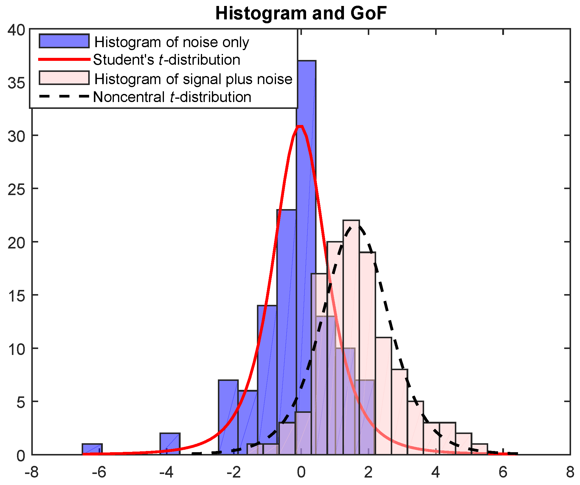
3.1. Statistical Model of the Collected Samples

We consider the case with a small number of samples and need to establish the test statistic model based on Student’s t-distribution. Hence, we further assume that the detected signal is a wide-band signal. As shown in [39], the bandwidth to be detected can be divided into n subbands, where each subband has equal bandwidth. For each subband, the m collected samples are limited to small numbers. Then, after receiving the samples at an SU, the samples X = { X i } i = 1 l are divided into n groups, with m ( m > 1 ) samples in each group, which indicates that n = l / m . The mean of the samples is defined as X j ¯ and the variance is S j 2 for the j-th group, respectively. Consequently, we can have
X j ¯ k = 0 m 1 X m j k m , S j 2 k = 0 m 1 ( X m j k X j ¯ ) 2 m 1
where j = 1 , 2 , , n and k = 0 , 1 , , m 1 . Let
Y j X j ¯ S j / m , j = 1 , 2 , , n .
Note that in order to calculate the following test statistic, the sequence { Y j } j = 1 n is sorted in increasing order and we assume that Y 1 Y 2 Y n .
Under H 0 hypothesis, PU transmits signal and the received samples follow X i N ( 0 , σ 2 ) . Then, Y j follows a v = m 1 degree Student’s t-distribution. In the case of the H 1 hypothesis, the transmitted signal and noise are both included in the received signal, it results that X i N ( μ , σ 2 ) , where μ = h . In this case, Y j is proved to follow a non-central Student’s t-distribution with degree of freedom given by v = m 1 and δ = m μ 2 / σ 2 , where μ 2 / σ 2 represents the signal-to-noise ratio (SNR) [32,50]. The histograms for different scenarios and GoFs of Y j for H 0 as well as H 1 hypotheses are shown in Figure 1, where SNR = 2 dB and the number of samples l = 64 . It can be observed from Figure 1 that the case with noise only fits the Student’s t-distribution well. Meanwhile, the case including both signal and noise matches the noncentral t-distribution curve. Moreover, for the same degree of freedom, we can notice that the noncentral t-distribution curve shifts slightly to the right side of the red curve of the Student’s t-distribution.
In addition, the curve shape of the Student’s t-distribution tends to approach a zero mean normal distribution with variance equal to 1. For parameter m, it can also be derived that the student’s t-distribution is closer to a standard normal distribution if m becomes larger. In contrast, if m gets smaller, the tails of the Student’s t-distribution tend to locate at a higher level as shown in Figure 2. Tails with different m values distribute at a higher level than that of the normal distribution,. Therefore, for small m, it indicates that variables Y j in Equation (16) tend to take values that deviate from their statistical mean. This could potentially result in inaccurate computation of the distance between the common cumulative distribution function and empirical distribution of the observation. Therefore, we need to accurately estimate the above distance in the next section.
It should be emphasized that the collected sample X i as Y j is reformulated and the Student’s t-distribution is satisfied with H 0 hypothesis while noncentral t-distribution is met for the H 1 hypothesis. Notice that for the H 0 hypothesis, the CDF F 0 ( y ) relates only with degrees of freedom v, while F 1 ( y ) depends on the term δ = m SNR . The noise variance σ 2 is also assumed to be known, which is the same assumption as ED-based methods. In addition, taking into account the limitations of the traditional GoF test (e.g.,AD test and KS test) under a small number of samples, we propose a likelihood ratio-based powerful statistic instead of the traditional statistic in the following section.

3.2. Powerful GoF Test

To precisely evaluate the distance between common CDF and the empirical distribution of the observation, a novel GoF test statistic Z c on the basis of the likelihood ratio is proposed. It is asymptotically equivalent to the Pearson χ 2 -statistic in Equation (4) under large sample situations. For obtaining the test statistic Z c , two kinds of statistic for testing H 0 with H 1 are defined by
Z = Z t d w ( t )
Z max = sup t ( , ) { Z t w ( t ) }
where Z t is the statistic for comparing H 0 ( t ) with H 1 ( t ) such that its large values reject H 0 ( t ) and w ( t ) is one of the weight functions. Note that
H 0 = t ( , ) H 0 ( t )
H 1 = t ( , ) H 1 ( t )
with H 0 ( t ) : F n ( t ) = F 0 ( t ) and H 1 ( t ) : F n ( t ) = F 1 ( t ) .
In [45], authors present a natural candidate for Z t , which is the likelihood ratio test statistic defined as follows:
G t 2 = 2 n [ F n ( t ) log { F n ( t ) F 0 ( t ) } + ( 1 F n ( t ) ) log { 1 F n ( t ) 1 F 0 ( t ) } ]
Setting Z t in Equation (17) equal to G t 2 and setting the weight function to a proper value d w ( t ) = F 0 ( t ) 1 { 1 F 0 ( t ) } 1 d F 0 ( t ) , we have
Z = j = 1 n [ l o g { F 0 ( y ) 1 1 } b i 1 + b i ] 2 + C n ,
where b i = i l o g ( i / n ) + ( n i ) l o g ( 1 i / n ) and C n is a constant value.
Since b i 1 b i l o g { ( n 1 2 ) / ( i 3 4 ) 1 } , we can derive the powerful GoF test statistic Z c 0 compared with the traditional GoF test. It is approximately obtained in the following
Z c 0 = j = 1 n [ log { F 0 ( y ) 1 1 ( n 1 / 2 ) / ( j 3 / 4 ) 1 } ] 2
where F 0 ( y ) denotes the CDF of Y j under H 0 hypothesis and it can be calculated by [50]:
F 0 ( y ) = 1 2 + 1 π tan 1 ( y ) , v = 1 , 1 2 + y 2 v + y 2 j = 0 ( v 2 ) / 2 b j ( 1 + y 2 v ) j , v e v e n , 1 2 + 1 π tan 1 ( y v ) + y v π ( v + y 2 ) j = 0 ( v 3 ) / 2 a j ( 1 + y 2 v ) j , v o d d ,
where a j = 2 j 2 j + 1 a j 1 , a 0 = 1 , b j = 2 j 1 2 j b j 1 , b 0 = 1 . In this situation, the statistic Z c 0 denotes the distance between the CDF of Y j under H 0 hypothesis and the empirical CDF of the collected samples. A large Z c 0 means that H 0 hypothesis is rejected with a large probability. Otherwise, a small Z c 0 means that the H 0 hypothesis is accepted. This is just the traditional GoF test, which is only based on the null hypothesis. However, in the proposed method, H 1 hypothesis is also considered to improve the reliability of the decision.
Therefore, corresponding to Equation (23), the other GoF test statistic Z c 1 based on H 1 hypothesis, is given as follows:
Z c 1 = j = 1 n [ log { F 1 ( y ) 1 1 ( n 1 / 2 ) / ( j 3 / 4 ) 1 } ] 2
where F 1 ( y ) denotes the CDF of Y j under H 1 hypothesis and it can be calculated by [50].
F 1 ( y ) = 1 2 j = 0 1 j ! ( δ 2 ) j e δ 2 2 Γ ( j + 1 2 ) π × I ( v v + y 2 ; v 2 , j + 1 2 ) , y 0 , 1 1 2 j = 0 1 j ! ( δ 2 ) j e δ 2 2 Γ ( j + 1 2 ) π × I ( v v + y 2 ; v 2 , j + 1 2 ) , y < 0 .
where Γ represents the gamma function and I denotes the regularized incomplete beta function. In this situation, the statistic Z c 1 denotes the distance between the CDF of Y j under H 1 hypothesis and the empirical CDF of the collected samples. A large Z c 1 means that H 1 hypothesis is rejected with a large probability. Otherwise, a small Z c 1 means that H 1 hypothesis is accepted.
In this section, due to adapting a more appropriate weight function, we derive a new GoF test statistic Z c 0 that is substantially more powerful than the traditional GoF test statistic under a small sample situation. Moreover, we further derive the other powerful GoF test statistic Z c 1 , which utilizes the CDF of noncentral t-distribution under H 1 hypothesis. At the end, in order to enhance the reliability of final decision, we propose to make a final decision based on bilateral hypotheses ( Z c 0 and Z c 1 ) in the next section.

3.3. Final Decision Based on Bilateral Hypotheses

In this section, we propose to make use of the information from bilateral hypotheses in order to more accurately detect the PU signal given a small number of received data. According to the statistical characteristic of the Student’s t-distribution and the noncentral t-distribution with different hypothesis in Section 3.1, and the two new powerful GoF test statistics Z c 0 in Equation (23) and Z c 1 in Equation (25) in Section 3.2, we make a final decision by comparing these two new GoF test statistics. Moreover, the normalization of the two GoF test statistics Z c 0 and Z c 1 can be written as T 0 = Z c 0 / ( Z c 0 + Z c 1 ) and T 1 = Z c 1 / ( Z c 0 + Z c 1 ) . Finally, the final decision can be determined based on the following rule:
H 0 : T 0 T 1 H 1 : T 1 < T 0 ,
where the information of bilateral hypotheses are both utilized to make a final decision, which significantly enhances the reliability of detection with small samples compared with the decision rule in Equation (13).

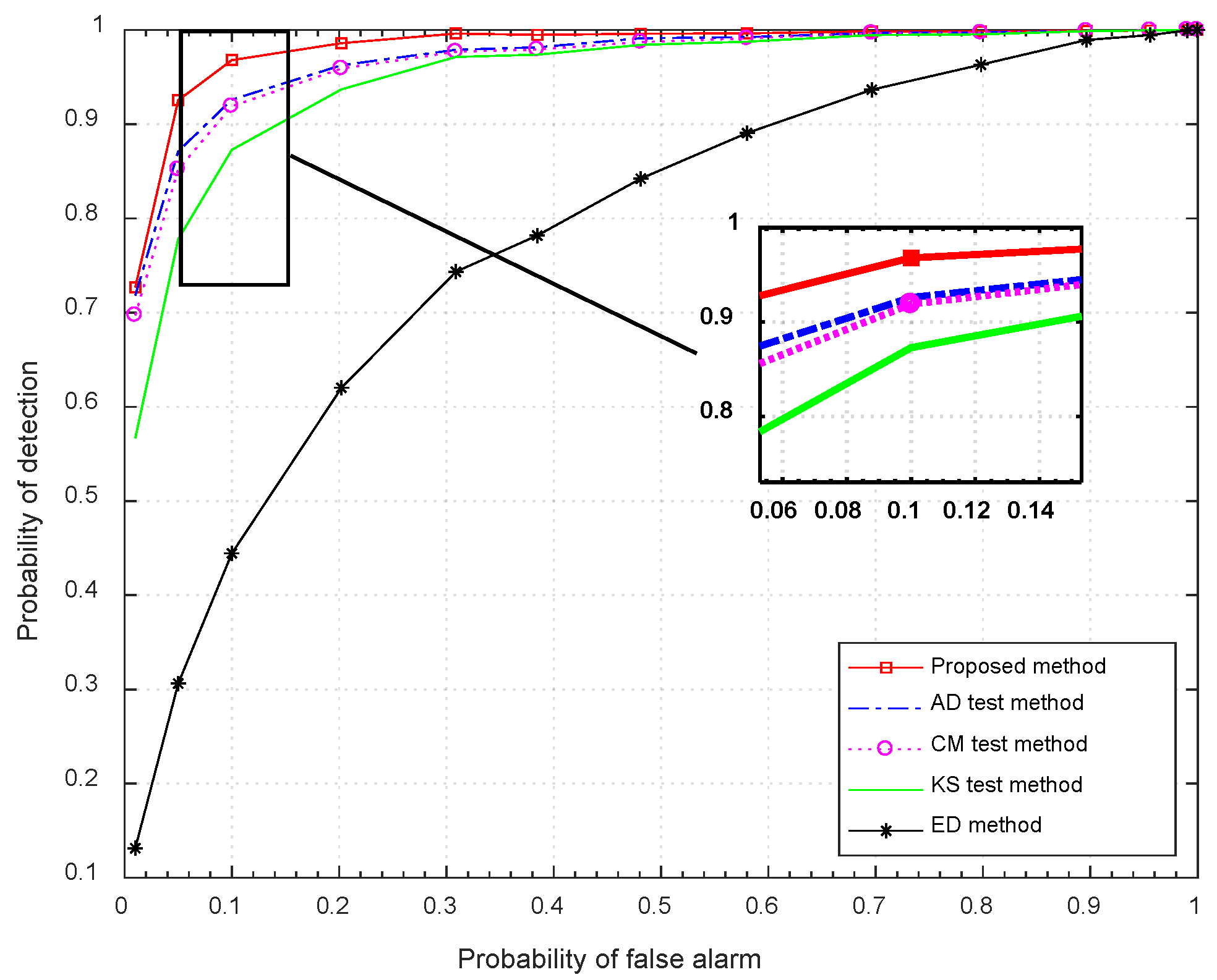
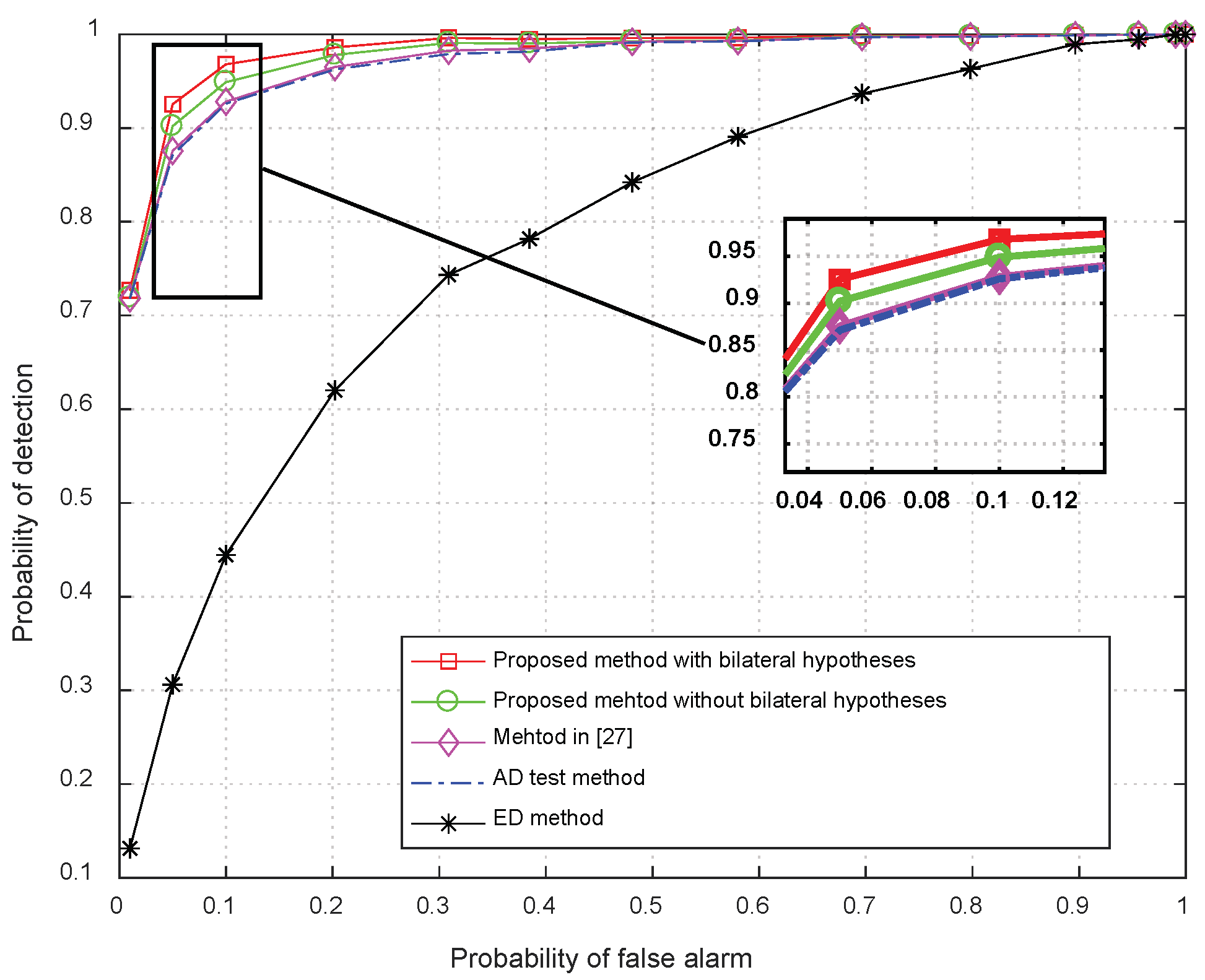
4. Simulation Results

In this section, the traditional GoF test (AD test, KS test, and CM test) based spectrum sensing methods and ED are considered for comparison. We assume that the PU signal is unknown while the noise power σ 2 is available in these methods.
First of all, to present the advantage of the proposed method, Figure 3 shows the detection probability providing different number of samples of the proposed method, AD test-based, KS test-based, and CM test-based method with the increasing of number of samples from 12 to 100 when P f a = 0.1 and the SNR is −5 dB. The parameter m is set to 4 for the proposed method. As shown in Figure 3, the proposed method surpasses the traditional GoF test-based spectrum sensing methods. Particularly, if the number of samples is smaller than 48, the proposed method has a big improvement of the detection probability compared to other techniques. In addition, Table 1 shows the detection probability of compared methods when the number of samples are 32, 40, and 48. We can see that the proposed method can achieve a detection probability of 0.9514 for SNR = −5 dB. It can also validate the robustness of proposed method.
Moreover, to compare the proposed method and other methods under different SNR conditions, the detection probability is provided in Figure 4 corresponding to the proposed method, the traditional GoF test based spectrum sensing methods and ED method with the increasing of SNR when P f a = 0.1 and the number of samples l = 32 . The parameter m is set to 4 for the proposed method. It can be seen from Figure 4 that the proposed scheme greatly surpasses the ED method. Importantly, the proposed method also has a better performance at low SNR region than the traditional GoF test (AD test, KS test, and CM test) based spectrum sensing methods. A specific example provided in Table 1 shows the detection probabilities corresponding to the l = 32 dotted lines in Figure 4 (SNR = −5 dB), which are 0.9514, 0.9206, 0.9070, and 0.8688 for the proposed method, AD test, CM test, and KS test, respectively. This also verifies that the proposed powerful GoF test method can achieve more reliable test statistic, leading to a better detection performance.
The receiver operating characteristic (ROC) curves are compared in Figure 5. It is obvious that the proposed method has better performance than the ED method. Given the probability of false alarm set to 0.1, SNR of −5 dB and l = 32 , the proposed method with m = 4 has about a 5% and 10% improvement relative to the AD test-based method and KS test-based method. That is because the proposed method utilizes the powerful GoF test statistic Z c that outperforms the traditional GoF test. For D 2 , W 2 , and A 2 in KS test, CM test, and AD test, it is difficult to find their exact null distributions for finite sample cases. In the powerful GoF test statistic Z c , we can use the sample mean and the sample variance to estimate μ and σ 2 , respectively, and it outperforms the best tests in the literature, including the KS test, CM test, and AD test [45].
In addition, in order to show the advantages of using the bilateral hypotheses to make the decision, we compare the proposed method with and without bilateral hypotheses, and a similar study using the GoF [27] in Figure 6. As shown in Figure 6, the performances of the proposed method with and without bilateral hypotheses are superior to the method in [27] and the AD test method. Moreover, the proposed method with bilateral hypotheses makes full use of the bilateral hypotheses information, which increases the utilization of the distribution properties. Thus, it has a higher probability of detection compared to the proposed method without bilateral hypotheses.

5. Conclusions

In this paper, an enhanced spectrum sensing method is proposed on the basis of a GoF test using bilateral hypotheses in a cognitive drone network. Only a small number of samples is required by the proposed scheme compared to the traditional ED, which is attractive for a dynamic weak signal scenario, including illegal drone detection. More specifically, samples at the SU with statistical model are thoroughly exploited, which strengthen its capacity for dealing with the small sample size case. Then, a powerful GoF test statistic Z c is proposed to obtain a better measurement, and bilateral hypotheses GoF test Z c 0 and Z c 1 are both used for making a reliable decision. Finally, simulations validate the superiority of the proposed method compared with the traditional GoF test-based methods (AD test, KS test, and CM test) and ED method provided a small number of samples. The capability of proposed method for settling small sample size problem without sacrificing the detection performance could bring several potential benefits, including sensing time, energy consumption, and computational burden to the whole drone network.

Author Contributions

Conceptualization and methodology, S.M. and Z.F., writing and validation, S.M., Z.F. and P.C. All authors have read and agreed to the published version of the manuscript.

Funding

This research was funded in part by the National Natural Science Foundation of China under Grant 82004259, in part by the GuangDong Basic and Applied Basic Research Foundation under Grant 2020A1515110503, in part by the Guangzhou Basic and Applied Basic Research Project under Grant 202102020674.

Institutional Review Board Statement

Not applicable.

Informed Consent Statement

Not applicable.

Data Availability Statement

Not applicable.

Conflicts of Interest

No conflict of interest exits in the submission of this manuscript, and the manuscript is approved by all authors for publication.

References

  1. Adamopoulos, E.; Rinaudo, F. UAS-Based Archaeological Remote Sensing: Review, Meta-Analysis and State-of-the-Art. Drones 2020, 4, 46. [Google Scholar] [CrossRef]
  2. Kaplan, B.; Kahraman, I.; Gorcin, A.; Çırpan, H.A.; Ekti, A.R. Measurement based FHSS–type Drone Controller Detection at 2.4GHz: An STFT Approach. In Proceedings of the 2020 IEEE 91st Vehicular Technology Conference (VTC2020-Spring), Antwerp, Belgium, 25–28 May 2020. [Google Scholar]
  3. Wang, D.; He, T.; Zhou, F.; Cheng, J.; Zhang, R.; Wu, Q. Outage-driven link selection for secure buffer-aided networks. Sci. China Inf. Sci. 2022, 65, 182303. [Google Scholar] [CrossRef]
  4. Wang, D.; Wu, M.; He, Y.; Pang, L.; Xu, Q.; Zhang, R. An HAP and UAVs Collaboration Framework for Uplink Secure Rate Maximization in NOMA-Enabled IoT Networks. Remote Sens. 2022, 14, 4501. [Google Scholar] [CrossRef]
  5. Ahmad, A.; Ahmad, S.; Rehmani, M.H.; Hassan, N.U. A Survey on Radio Resource Allocation in Cognitive Radio Sensor Networks. IEEE Commun. Surv. Tuts. 2015, 17, 888–917. [Google Scholar] [CrossRef]
  6. Chen, X.; Chen, H.; Meng, W. Cooperative communications for cognitive radio networks from theory to applications. IEEE Commun. Surv. Tuts. 2014, 16, 1180–1192. [Google Scholar] [CrossRef]
  7. Kakalou, I.; Psannis, K.E.; Krawiec, P.; Badea, R. Cognitive radio network and network service chaining toward 5g: Challenges and requirements. IEEE Commun. Mag. 2017, 55, 145–151. [Google Scholar] [CrossRef]
  8. Liang, W.; Ng, S.X.; Hanzo, L. Cooperative overlay spectrum access in cognitive radio networks. IEEE Commun. Surv. Tuts. 2017, 19, 1924–1944. [Google Scholar] [CrossRef] [Green Version]
  9. Hefnawi, M. Large-Scale Multi-Cluster MIMO Approach for Cognitive Radio Sensor Networks. IEEE Sens. J. 2016, 16, 4418–4424. [Google Scholar] [CrossRef]
  10. Akan, O.B.; Karli, O.B.; Ergul, O. Cognitive radio sensor networks. IEEE Netw. 2009, 23, 34–40. [Google Scholar] [CrossRef]
  11. Joshi, G.P.; Nam, S.Y.; Kim, S.W. Cognitive radio wireless sensor networks: Applications, challenges and research trends. Sensors 2013, 13, 11196–11228. [Google Scholar] [CrossRef]
  12. Wang, D.; Zhou, F.; Lin, W.; Ding, Z.; Dhahir, N.A. Cooperative Hybrid Non-Orthogonal Multiple Access Based Mobile-Edge Computing in Cognitive Radio Networks. IEEE Trans. Cogn. Commun. Netw. 2022, 8, 1104–1117. [Google Scholar] [CrossRef]
  13. Ali, A.; Hamouda, W. Advances on Spectrum Sensing for Cognitive Radio Networks: Theory and Applications. IEEE Commun. Surv. Tuts. 2017, 19, 1277–1304. [Google Scholar] [CrossRef]
  14. Axell, E.; Leus, G.; Larsson, E.G.; Poor, H.V. Spectrum sensing for cognitive radio: State-of-the-art and recent advances. IEEE Signal Process. Mag. 2012, 29, 101–116. [Google Scholar] [CrossRef] [Green Version]
  15. Cicho, K.; Kliks, A.; Bogucka, H. Energy-Efficient Cooperative Spectrum Sensing: A Survey. IEEE Commun. Surv. Tuts. 2016, 18, 1861–1886. [Google Scholar] [CrossRef]
  16. Yücek, T.; Arslan, H. A survey of spectrum sensing algorithms for cognitive radio applications. IEEE Commun. Surv. Tuts. 2009, 11, 116–130. [Google Scholar] [CrossRef]
  17. Wang, B.; Liu, K.J. Advances in cognitive radio networks: A survey. IEEE J. Sel. Top. Signal Process. 2011, 5, 5–23. [Google Scholar] [CrossRef] [Green Version]
  18. Urkowitz, H. Energy detection of unknown deterministic signals. Proc. IEEE 1967, 55, 523–531. [Google Scholar] [CrossRef]
  19. Sofotasios, P.C.; Rebeiz, E.; Tsiftsis, L.Z.T.A.; Cabric, D.; Freear, S. Energy Detection Based Spectrum Sensing Overκμ and κμExtreme Fading Channels. IEEE Trans. Veh. Technol. 2013, 62, 1031–1040. [Google Scholar] [CrossRef]
  20. Chatziantonious, E.; Allen, B.; Velisavljevic, V.; Karadimas, P.; Coon, J. Energy Detection Based Spectrum Sensing Over Two-Wave With Diffuse Power Fading Channels. IEEE Trans. Veh. Technol. 2017, 66, 868–874. [Google Scholar]
  21. Zeng, Y.; Liang, Y.C. Eigenvalue-based spectrum sensing algorithms for cognitive radio. IEEE Trans. Commun. 2009, 57, 1784–1793. [Google Scholar] [CrossRef] [Green Version]
  22. Tsinos, C.G.; Berberidis, K. Decentralized Adaptive Eigenvalue-Based Spectrum Sensing for Multiantenna Cognitive Radio Systems. IEEE Trans. Wireless Commun. 2015, 14, 1703–1715. [Google Scholar] [CrossRef]
  23. Bouallegue, K.; Dayoub, I.; Gharbi, M.; Hassan, K. Blind Spectrum Sensing Using Extreme Eigenvalues for Cognitive Radio Networks. IEEE Commun. Lett. 2018, 2, 1386–1389. [Google Scholar] [CrossRef]
  24. Nguyen-Thanh, N.; Kieu-Xuan, T.; Koo, I. Comments and Corrections Comments on “Spectrum Sensing in Cognitive Radio Using Goodness-of-Fit Testing”. IEEE Trans. Wirel. Commun. 2012, 11, 3409–3411. [Google Scholar] [CrossRef]
  25. Teguig, D.; Nir, V.L.; Scheers, B. Spectrum sensing method based on goodness of fit test using chi-square distribution. Electron. Lett. 2014, 50, 713–715. [Google Scholar] [CrossRef] [Green Version]
  26. Teguig, D.; Nir, V.L.; Scheers, B. Spectrum sensing Method Based on the Likelihood Ratio Goodness of Fit test under noise uncertainty. Electron. Lett. 2015, 51, 253–255. [Google Scholar] [CrossRef] [Green Version]
  27. Scheers, B.; Teguig, D.; Nir, V.L. Wideband spectrum sensing technique based on Goodness-of-Fit testing. In Proceedings of the 2015 International Conference on Military Communications and Information Systems (ICMCIS), Cracow, Poland, 16 July 2015; pp. 1–6. [Google Scholar] [CrossRef]
  28. Jin, M.; Guo, Q.; Xi, J.; Yu, Y. Spectrum sensing based on goodness of fit test with unilateral alternative hypothesis. Electron. Lett. 2014, 50, 1645–1646. [Google Scholar] [CrossRef]
  29. Kockaya, K.; Develi, I. Spectrum sensing in cognitive radio networks: Threshold optimization and analysis. J. Wirel. Com Netw. 2020, 2020, 255. [Google Scholar] [CrossRef]
  30. Gai, J.; Zhang, L.; Wei, Z. Spectrum Sensing Based on STFT-ImpResNet for Cognitive Radio. Electronics 2022, 11, 2437. [Google Scholar] [CrossRef]
  31. Wang, H.; Yang, E.H.; Zhao, Z.; Zhang, W. Spectrum sensing in cognitive radio using goodness of fit testing. IEEE Trans. Wirel. Commun. 2009, 8, 5427–5430. [Google Scholar] [CrossRef]
  32. Shen, L.; Wang, H.; Zhang, W.; Zhao, Z. Blind spectrum sensing for cognitive radio channels with noise uncertainty. IEEE Trans. Wirel. Commun. 2011, 10, 1721–1724. [Google Scholar] [CrossRef]
  33. Zhang, G.; Wang, X.; Liang, Y.C.; Liu, J. Fast and robust spectrum sensing via Kolmogorov-Smirnov test. IEEE Trans. Commun. 2010, 58, 3410–3416. [Google Scholar] [CrossRef]
  34. Patel, D.K.; Trivedi, Y.N. Goodness-of-fit-based non-parametric spectrum sensing under Middleton noise for cognitive radio. Electron. Lett. 2015, 51, 419–421. [Google Scholar] [CrossRef]
  35. Ye, Y.; Lu, G.; Li, Y.; Jin, M. Unilateral right-tail Anderson-Darling test based spectrum sensing for cognitive radio. Electron. Lett. 2017, 53, 1256–1258. [Google Scholar] [CrossRef]
  36. Liu, C.; Wang, J.; Liu, X.; Liang, Y. Maximum Eigenvalue-Based Goodness-of-Fit Detection for Spectrum Sensing in Cognitive Radio. IEEE Trans. Veh. Technol. 2019, 68, 7747–7760. [Google Scholar] [CrossRef]
  37. Rugini, L.; Banelli, P.; Leus, G. Small sample size performance of the energy detector. IEEE Commun. Lett. 2013, 17, 1814–1817. [Google Scholar] [CrossRef] [Green Version]
  38. Arshad, K.; Moessner, K. Robust spectrum sensing based on statistical tests. IET Commun. 2013, 7, 808–817. [Google Scholar] [CrossRef] [Green Version]
  39. Men, S.; Chargé, P.; Wang, Y.; Li, J. Wideband signal detection for cognitive radio applications with limited resources. Eurasip J. Adv. Signal Process. 2019, 2019, 1–10. [Google Scholar] [CrossRef] [Green Version]
  40. Rostami, S.; Arshad, K.; Moessner, K. Order-statistic based spectrum sensing for cognitive radio. IEEE Commun. Lett. 2012, 16, 592–595. [Google Scholar] [CrossRef] [Green Version]
  41. Denkovski, D.; Atanasovski, V.; Gavrilovska, L. HOS Based Goodness-of-Fit Testing Signal Detection. IEEE Commun. Lett. 2012, 16, 310–313. [Google Scholar] [CrossRef]
  42. Pakyari, R.; Balakrishnan, N. A General Purpose Approximate Goodness-of-Fit Test for Progressively Type-II Censored Data. IEEE Trans. Reliab. 2012, 61, 238–244. [Google Scholar] [CrossRef]
  43. Noughabi, H.A.; Balakrishnan, N. Goodness of Fit Using a New Estimate of Kullback-Leibler Information Based on Type II Censored Data. IEEE Trans. Reliab. 2015, 64, 627–635. [Google Scholar] [CrossRef]
  44. Qiu, Y.; Liu, L.; Lai, X.; Qiu, Y. An Online Test for Goodness-of-Fit in Logistic Regression Model. IEEE Access 2019, 7, 107179–107187. [Google Scholar] [CrossRef]
  45. Zhang, J. Powerful goodness-of-fit tests based on the likelihood ratio. J. Roy. Statist. Soc. Ser. B 2002, 64, 281–294. [Google Scholar] [CrossRef]
  46. Terry, K.; Agostino, R.B.; Stephens, M.A. Goodness-of-Fit Techniques. Technometrics 1987, 29, 493. [Google Scholar]
  47. Stephens, M.A. EDF statistics for goodness of fit and some comparisons. J. Amer. Statist. Assoc. 1974, 69, 730–737. [Google Scholar] [CrossRef]
  48. Anderson, T.W.; Darling, D.A. Asymptotic theory of certai “goodness of fit” criteria based on stochastic processes. Ann. Math. Stat. 1952, 23, 193–212. [Google Scholar] [CrossRef]
  49. Stephens, M.A. Use of the Kolmogorov-Smirnov, Cramer-Von Mises and Related Statistics Without Extensive Tables. J. R. Stat. Soc. Ser. B 1970, 32, 115–122. [Google Scholar] [CrossRef]
  50. Forbes, C.; Evans, M.; Hastings, N.; Peacock, B. Statistical Distributions; John Wiley: Hoboken, NJ, USA, 2011. [Google Scholar]
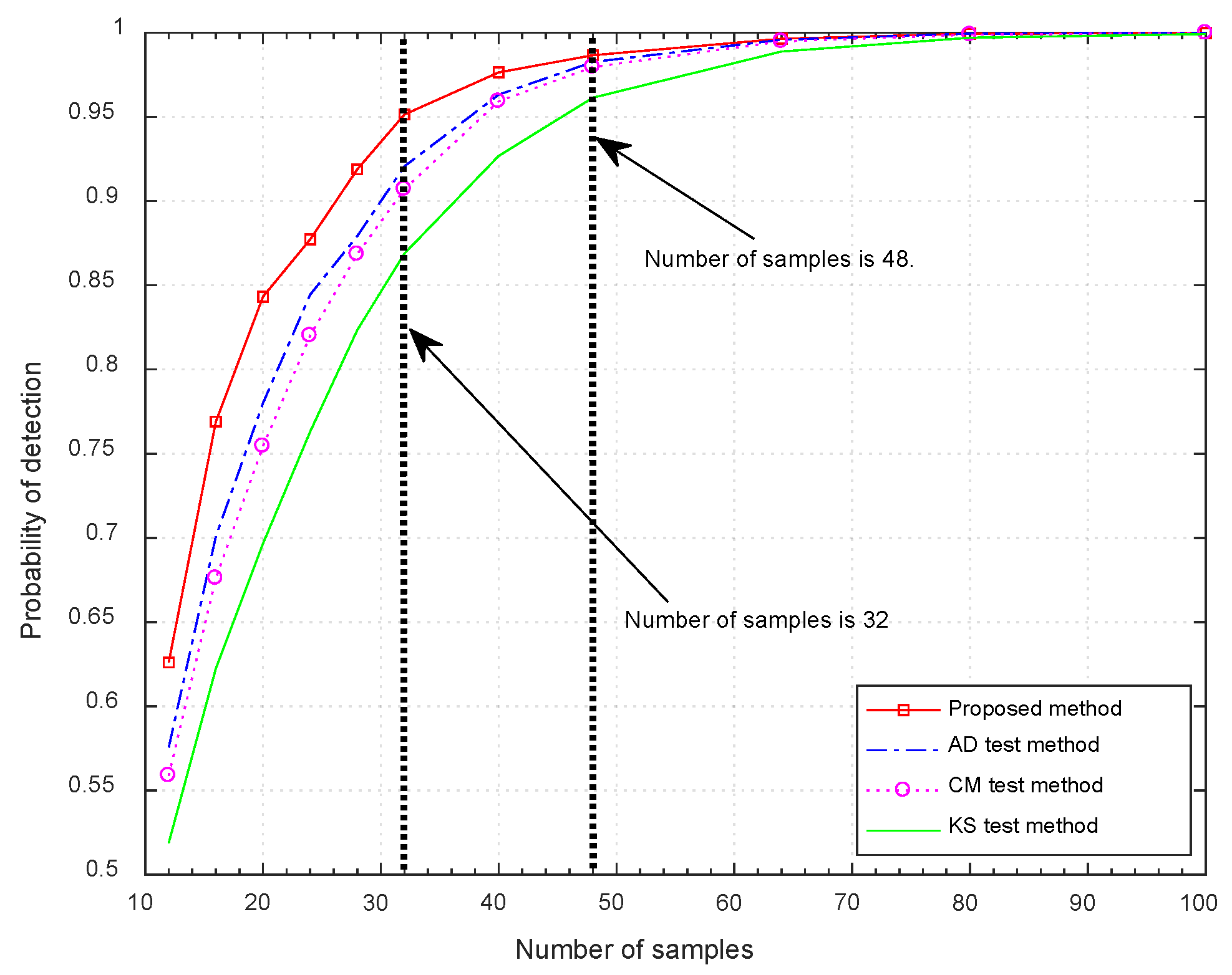
Figure 1. Histogram for scenarios with signal and without signal, GoF of Y j under different hypotheses.
Drones 07 00018 g001
Figure 2. Probability density function (PDF) with different degrees of freedom v = m 1 in Student’s t-distribution.
Drones 07 00018 g002
Figure 3. Probability of detection with different number of samples over AWGN channels with P f a = 0.1 .
Drones 07 00018 g003
Figure 4. Detection probability with different SNR over AWGN channels with P f a = 0.1 .
Drones 07 00018 g004
Figure 5. ROC curves comparison with SNR = −5 dB.
Drones 07 00018 g005
Figure 6. ROC curves comparison with SNR = −5 dB.
Drones 07 00018 g006
Table 1. The probability of detection for different methods when the number of samples are 32, 40, and 48.
Number of SamplesKS Test MethodCM Test MethodAD Test MethodProposed Method
320.86880.90700.92060.9514
400.92680.95920.96320.9764
480.96140.97960.98260.9866
Disclaimer/Publisher’s Note: The statements, opinions and data contained in all publications are solely those of the individual author(s) and contributor(s) and not of MDPI and/or the editor(s). MDPI and/or the editor(s) disclaim responsibility for any injury to people or property resulting from any ideas, methods, instructions or products referred to in the content.

