Article

Practically Robust Fixed-Time Convergent Sliding Mode Control for Underactuated Aerial Flexible JointRobots Manipulators

1
Faculty of Science, Engineering and Technology, Swinburne University of Technology, Melbourne 3122, Australia
2
Department of Automated Manufacturing, Al Khwarizmi College of Engineering, University of Baghdad, Baghdad 10071, Iraq
3
Biomedical Device Innovation Center, Shenzhen Technology University, Shenzhen 518118, China
4
Department of Chemical & Materials Engineering, University of Auckland, Auckland 1010, New Zealand
*
Author to whom correspondence should be addressed.
Drones 2022, 6(12), 428; https://doi.org/10.3390/drones6120428
Submission received: 27 October 2022 / Revised: 16 December 2022 / Accepted: 16 December 2022 / Published: 19 December 2022
(This article belongs to the Special Issue Bioinspiration, Biomimicry, and Soft Robotics of Drones)

Abstract

:
The control of an aerial flexible joint robot (FJR) manipulator system with underactuation is a difficult task due to unavoidable factors, including, coupling, underactuation, nonlinearities, unmodeled uncertainties, and unpredictable external disturbances. To mitigate those issues, a new robust fixed-time sliding mode control (FxTSMC) is proposed by using a fixed-time sliding mode observer (FxTSMO) for the trajectory tracking problem of the FJR attached to the drones system. First, the underactuated FJR is comprehensively modeled and converted to a canonical model by employing two state transformations for ease of the control design. Then, based on the availability of the measured states, a cascaded FxTSMO (CFxTSMO) is constructed to estimate the unmeasurable variables and lumped disturbances simultaneously in fixed-time, and to effectively reduce the estimation noise. Finally, the FxTSMC scheme for a high-order underactuated FJR system is designed to guarantee that the system tracking error approaches to zero within a fixed-time that is independent of the initial conditions. The fixed-time stability of the closed-loop system of the FJR dynamics is mathematically proven by the Lyapunov theorem. Simulation investigations and hardware tests are performed to demonstrate the efficiency of the proposed controller scheme. Furthermore, the control technique developed in this research could be implemented to the various underactuated mechanical systems (UMSs), like drones, in a promising way.

1. Introduction

Recently, the research on the trajectory tracking control of the FJR has gained much more consideration due to its merits such as lightweight, high maneuverability, backdrivability, low energy consumption, and so on [1]. Still, designing a robust control law for the FJR system with high motion performance is a huge and challenging mission for researchers in the control community due to inherent system properties. First, the system order becomes double in the presence of joint flexibility, which reflects the model and control design complexity [2]. Second, a strong coupling exists between the motor and the link via torsional springs, illustrating that the FJR system is underactuated, in which the number of control inputs is lower than the number of outputs to be controlled. Third, the control performance FJR often seriously suffers from unfavorable factors such as parametric uncertainties, unstructured dynamics, non linearities, and unknown perturbations. Fourth, residual vibration may degrade the control characters such as settling time, rising time, and overshoot, and this may even lead to mechanical damage.
In the existing literature on the tracking controller design of the FJR system, there have been numerous attempts to address the above issues, including PID, passivity-based control, adaptive control, singular perturbation control, backstepping, and sliding mode control, etc. [2,3,4,5,6,7,8,9,10,11,12,13,14,15,16,17,18,19]. Among them, the sliding mode control (SMC) has proven its reputation in control engineering society owing to its robust performance against system uncertainties and perturbations [14,15,20,21]. Although existing SMC schemes have asymptotic and fast finite-time convergence, they are sensitive to the system state’s initial conditions. To cope with this issue, the fixed-time SMC (FxTSMC) has been proposed [22], which is adopted in this paper for an uncertain high-order FJR system.
In addition, the chattering reduction and the lumped disturbance bound relaxation are generally important perspectives for the SMC method. These are achieved by incorporating the SMC with disturbance observer techniques. Many existing observers have been previously reported in the literature [14,15,21] for the FJR system. Furthermore, the extended state observer (ESO) has been proven as being a promising observer tool in the active disturbance rejection control techniques for estimating states and disturbance, which have been applied for different systems such as drones [23,24]. However, the estimation error of the states and disturbances in the above observer works can only approach to zero asymptotically and slowly, and they are sensitive to the initial conditions. In reality, the convergence speed of such observers greatly affects the control effectiveness of the FJR plant. To further enhance the observation equality, the current paper proposes a fixed-time slide mode observer (FxTSMO) featured with bounded settling time, irregardless of the initial conditions for an underactuated FJR to estimate unmeasurable states and lumped disturbances accurately. Moreover, the cascaded fixed-time sliding mode observer (CFxTSMO) is adopted to reduce the estimation noise and peaking phenomena in the estimations, which are critical in the hardware implementation of a high-order system.
The proposed algorithm makes the following contributions:
(i)
The integrated dynamic modeling of the underactuated FJR system is well established, and the detailed analysis is also given. By using the Olfati and flatness transformation, the established FJR dynamic model is converted into a canonical representation, which then is cascaded due to two available states. Thus, the coupling issue in the control input of the underactuated FJR system is handled through these transformations. Accordingly, no linearization nor approximation are needed due to the fact that the FJR system in practice has inevitably complex nonlinearities caused by flexibility, friction, and other sources.
(ii)
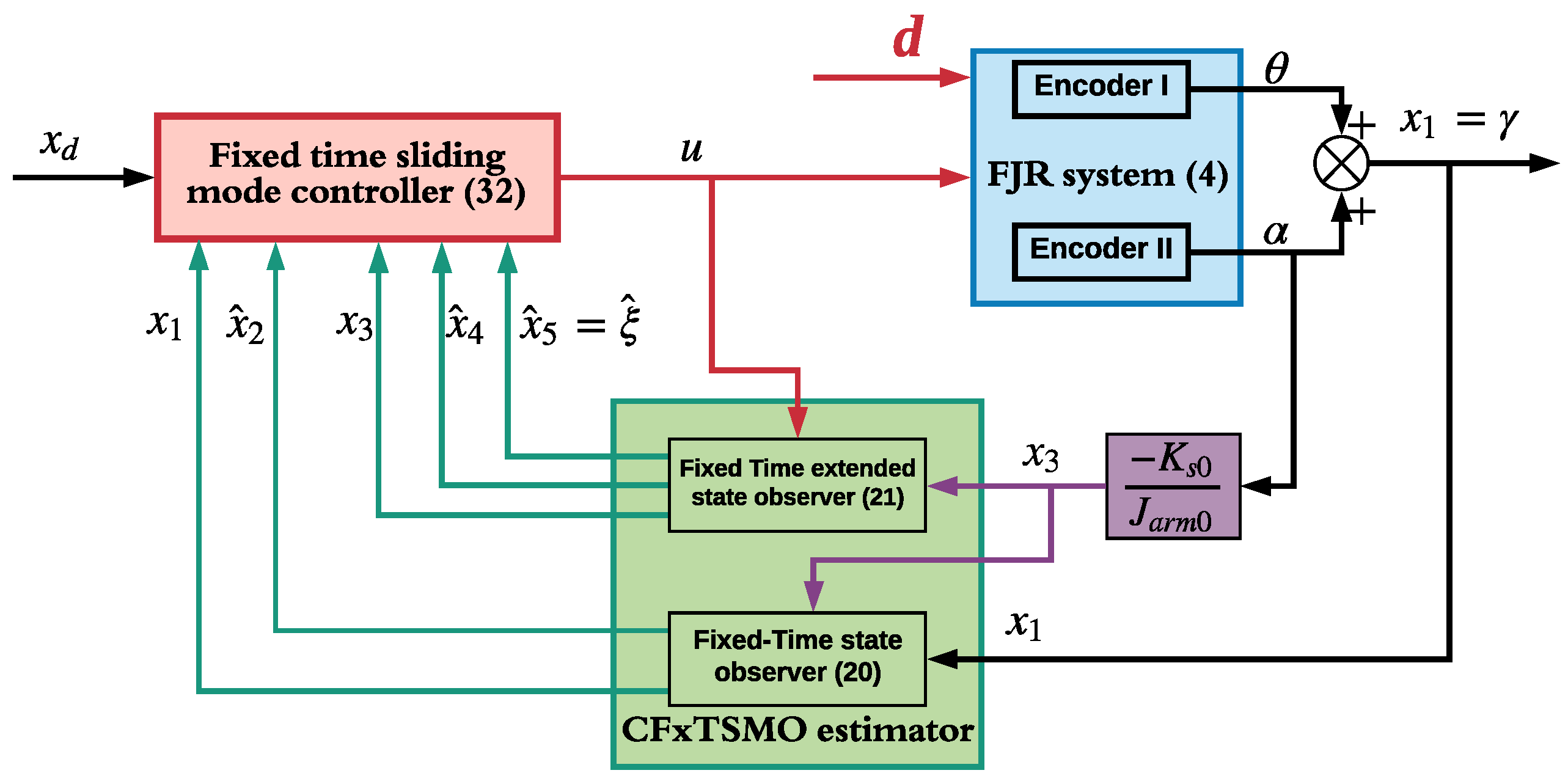
The CFxTSMO is constructed based on the cascaded structure to greatly smooth out the measurement noise in the fixed-time estimates of unknown states and disturbances, which makes the FxTSMC scheme feasible for the real FJR system. Via the aid of such smooth estimations, a fixed-time sliding surface is newly designed to ensure a fixed-time convergence, which needs a partial knowledge of the estimation states, including the velocity and jerk signal, whereas a position and an acceleration signal can be measured.
(iii)
Unlike the existing finite-time convergent controller works [20,25] for fourth-order systems, the proposed FxTSMC controller for the FJR system with fourth-order practically guarantees not only fixed-time convergence, even in the presence of the initial conditions, but it also ensures a total robustness against disturbances and estimation error.
(iv)
The fixed-time stability of the whole closed-loop FJR plant is theoretically proven. Compared with some simulations works of fixed-time SMC schemes [26,27,28,29,30], the proposed control scheme is practically validated on the actual FJR system. Extensive simulations and persuasive experimental results are provided to show its tracking efficiency and robustness performance against disturbances and initial conditions. To the best of our knowledge, the proposed CFxTSMO-based FxTSMC scheme is reported here for the first time in the open literature for the FJR system and underactuated mechanical systems (UMSs). This study presents our controller as a good control candidate for other kinds of UMSs, including drone systems.
The following is the organization of the rest of the work. The mathematical model of the FJR plant, as well as the coordinates transformation, are presented in Section 2. The proposed controller and observer, and their corresponding stability proofs, are analyzed in Section 3. In Section 4, the numerical simulations and experimental results validating the performance of proposed controllers for the real FJR system are provided. In the last, some concluding remarks wrap up this article in Section 5.

2. Dynamic Modeling

2.1. Description of the Single-Link FJR System

The fly robot arm is amounted to many drones to perform handling and unhandling tasks, which can be can considered as the FJR system. In this work, we will study the FJR system under the motion of drones. The FJR system shown in Figure 1 is made up of two similar springs, a DC motor, an aluminum chassis, two encoders, a free rigid link, and a set of gear speed reduction. The driving torque for this device is transmitted from the DC motor to the system link via the gearbox and the springs, according to its operating principle. Unfortunately, the flexibility of these springs causes the link to vibrate, which can negatively impact upon the performance of the link movement.
The basic sketch of the FJR system attached to the drones is presented in Figure 1 to show the main coordinates with which the FJR can be characterized in the dynamic modeling. As illustrated in Figure 1, the variables α and θ are the link deflection angle and the motor position angle, respectively, which can be read by two encoders, respectively. The summation of α and θ is the overall link tip position angle denoted by γ .

2.2. FJR Dynamic Modeling

In the introduction of high gear reduction and other elastic mechanisms, as in reality, the FJR dynamics consist of two sides coupled by the joint flexibility, that is, the link side dynamics [21]
α ¨ t a 1 α t a 3 θ ˙ t = b 1 u t
and motor side dynamics
θ ¨ t a 2 α t a 4 θ ˙ t = b 2 u t
with
a 1 = K s J e q + J a r m J e q J a r m ; a 2 = K s J e q ; a 3 = η m η g K t K m K g 2 + B e q R m J e q R m ; a 4 = a 3 ; b 1 = η m η g K t K g J e q R m ; b 2 = b 1
where the descriptions and typical values of all involved quantities appearing in (1) and (2) are: J a r m ( 0.0019 kg . m 2 ) and J e q ( 0.0021 kg . m 2 ) are the inertia of the arm and the equivalent motor, respectively; K s ( 1.2485 N.m/rad) is the joint stiffness, B e q (0.004 N.m.s/rad) is the equivalent viscous friction coefficient, R m ( 2.6 Ω ) is the armature resistance, K m ( 0.00767   V . s / rad ) is the motor back-EMF constant, K t ( 0.00767 N . m / A ) is the constant of motor torque, K g (14:5) is the high gear ratio, η g ( 0.9 ) and η m ( 0.69 ) are the efficiencies of the gearbox and motor, respectively; and u stands for the control voltage, which will be produced by the proposed control scheme.
In the current paper, taking the parameters variations into account in both the motor and the link element, we formulate the parametric uncertainties with their upper-bounds, as follows:
J e q = J e q J e q 0 ¯ J e q J a r m = J a r m J a r m 0 ¯ J a r m K s = K s K s 0 ¯ K s B e q = B e q B e q 0 ¯ B e q
where J e q 0 , J a r m 0 , K s 0 and B e q 0 represent the nominal parameters of the FJR system as given above; J e q 0 , J a r m , K s 0 , and B e q 0 denote the parametric uncertainties; and ¯ B e q , ¯ J a r m , ¯ K s , and ¯ J e q stand for the upper-bounds of the corresponding parameters.
Let us define the FJR system state vector as η = [ η 1 , η 2 , η 3 , η 4 ] T = [ α , α ˙ , θ , θ ˙ ] T . Using the nominal plant and considering parametric uncertainties, external perturbations, and nonlinearities resulting from the flexibility and friction, the state–space form of the overall dynamic of the FJR system in (1) and (2) is described as follows:
Link subsystem η ˙ 1 ( t ) = η 2 ( t ) η ˙ 2 ( t ) = f 10 ( η ) + b 10 u + τ dl ( η , u , w l ) + O sp ( α ) Motor subsystem η ˙ 3 ( t ) = η 4 ( t ) η ˙ 4 ( t ) = f 20 ( η ) + b 20 u + τ dm ( η , u , w m ) + O sp , fric ( α , θ ˙ ) System output η o ( t ) = η 1 ( t ) = α ( t ) , η 3 ( t ) = θ ( t ) T
where the output state vector η o ( t ) has α ( t ) and θ ( t ) , which are available for measurement; f 10 ( η ) and f 20 ( η ) are the nominal functions of the motor and link subsystem, respectively, described as
f 10 ( η ) = a 10 α t + a 30 θ ˙ t f 20 ( η ) = a 20 α t + a 40 θ ˙ t .
τ dl ( η , u , w l ) and τ dm ( η , u , w m ) are the lumped disturbances of both subsystem dynamics, which are given by
τ dl ( η , u , w l ) = f 1 ( η ) + b 1 u + w l ( η , t ) τ dm ( η , u , w m ) = f 2 ( η ) + b 2 u ( t ) + w m ( η , t )
where w l ( η , t ) and w m ( η , t ) are the unmodeled dynamics and external disturbances acting on both dynamics; f 1 ( η ) and f 2 ( η ) are the terms of parametric uncertainty multiplied by states in both the subsystem functions f 1 ( η ) and f 2 ( η ) , respectively, which are defined as
f 1 ( η ) = a 1 α t + a 3 θ ˙ t f 2 ( η ) = a 2 α t + a 4 θ ˙ t .
Furthermore, O sp ( α ) and O sp , fric ( α , θ ˙ ) in (4) are high-order nonlinear terms of the link and motor dynamics due to flexibility and friction. To capture the nonlinearity caused by the flexibility, since the relationship of spring torque-deflection is nonlinear in practice, the total spring torque of the elastic mechanism (such as gears, brings, tendons, etc.) is described by
τ sp = K s α + K s n α 3 ; K s > 0
where K s denotes the known spring coefficient associated with the linear part; K s n indicates the constant associated with the (cubic) nonlinearity. Based on the value of K s n , the spring becomes hard if K s n > 0 , linear if K s n = 0 , and soft if K s n < 0 . From (8), the unknown cubic nonlinearity of the spring is treated as a high-nonlinear term O sp ( α ) , and (8) becomes
τ sp = K s α + O sp ( α )
in which its first term is already covered in the differential Equations (1) and (2), while the second term is considered in (4).
Concerning friction nonlinearities; this is because the friction model in the motor drive side consists of viscous and Coulomb terms, for an example. To capture the nonlinear friction behavior, the total friction torque of the motor, along with a speed operation θ ˙ , is described by
τ fric = B e q θ ˙ + F c sign ( θ ˙ )
where B e q is the linear viscous friction coefficient as defined with the system parameters, and F c > 0 denotes the Coulomb friction coefficient associated with the nonlinear part, which is unknown. By defining the unknown friction nonlinearity F c sign ( θ ˙ ) as the nonlinear friction term O fric ( θ ˙ ) , the friction model (10) can be rewritten as
τ fric = B e q θ ˙ + O fric ( θ ˙ )
in which the first term is already included in the motor subsystem dynamics in (2) and the second complex nonlinearity term is combined with O sp ( α ) to constitute the total nonlinearity O sp , fric ( α , θ ˙ ) of the motor drive dynamics (4), as follows:
O sp , fric ( α , θ ˙ ) = K s n α 3 + F c sign ( θ ˙ ) .

2.3. State Transformation Procedure of the Underactuated FJR Manipulator

To get rid of the underactuation and coupling issue in the FJR system (4), the Olfati’s global coordinate transformation [31] is used as follows
z 1 ( t ) = η 1 ( t ) 0 η 3 b 10 b 20 d s = η 1 ( t ) + η 3 ( t ) z 2 ( t ) = η 2 ( t ) b 10 b 20 η 4 ( t ) = η 2 ( t ) + η 4 ( t ) z 3 ( t ) = η 3 ( t ) z 4 ( t ) = η 4 ( t )
where
b 10 = η m η g K t K g J e q 0 R m ; b 20 = b 10 .
By differentiating (13) by substituting the coupled underactuated FJR (4), the original FJR system (4) is converted into the following decoupled FJR model in a cascade form as
z ˙ 1 ( t ) = z 2 ( t ) z ˙ 2 ( t ) = z 3 + d u ( z , w l , w m ) z ˙ 3 ( t ) = z 4 ( t ) z ˙ 4 ( t ) = f 2 ( α , θ ˙ ) + b 2 u + d m ( z , u , w m )
with
d u ( z , w l , w m ) = z 3 + f 10 ( z ) + f 20 ( z ) + τ d l + τ d m + O sp + O sp , fric ; = z 3 + ( a 10 + a 20 ) ( z 1 z 3 ) + τ d l m + O u ; where τ d l m = τ d l + τ d m ; O u = O sp + O sp , fric d m ( z , u , w m ) = τ d m + O m and O m = O sp , fric
where z = [ z 1 ( t ) = γ ( t ) , z 2 ( t ) = γ ˙ ( t ) , z 3 ( t ) = θ ( t ) , z 4 ( t ) = θ ˙ ( t ) ] T is the state vector in the new Z-space; d u and d m are the state-dependent unmatched and matched disturbances, respectively. O u and O m denote the state-dependent unmatched and matched nonlinearities.
In order to make the controller design of (14) more manageable, the mismatched disturbance d u ( z , w l , w m ) is turned out to the matched one by utilizing the flatness method [32]. Based on this method, the output z 1 ( t ) of dynamics (14) is differentiated four times, since the FJR system possesses the four relative degree. Accordingly, let the new states as x 1 t = z 1 ( t ) , x 2 ( t ) = z ˙ 1 ( t ) , x 3 t = z ¨ 1 ( t ) and x 4 ( t ) = z 1 ( t ) be defined; the flatness method allows us to explicitly obtain the following input–output differential equation as
x ˙ 1 ( t ) = x 2 ( t ) x ˙ 2 ( t ) = x 3 ( t ) x ˙ 3 ( t ) = x 4 ( t ) x ˙ 4 ( t ) = b 0 u ( t ) + ξ ( x , u , d ) y t = x 1 t
with
b 0 = η m η g K t K g K s 0 J a r m 0 J e q 0 R m
which represents a single-input-single output (SISO) dynamics with the new phase variable vector x = [ x 1 = γ , x 2 = γ ˙ , x 3 = γ ¨ , x 4 = γ ] T , including the displacement, velocity, and jerk signal of the rigid link. As shown in (15), an overall matched disturbance ξ ( x , u , d ) acting on the SISO FJR plant may include many elements, i.e., the dynamics of nominal motor and manipulator, unstructured dynamics, parametric uncertainties, external disturbances, and nonlinearities caused by the flexibility and other sources, and it is mathematically defined as follows
ξ ( x , u , d ) = a 30 x 1 + a 10 x ¨ 1 + K s 0 a 30 J a r m 0 x ˙ 1 FJR manipulator dynamics + d ( x , u , w ) state-dependent uncertainties + O ( x , u ) state and input-dependent nonlinearities
with
d ( x , u , w ) = τ ¨ d l m ( η , u , w l , w m ) + τ d m η , u , w m , O ( x ) = O ¨ u ( x ) + O m ( x ) .
For the simplified form (15), the basis control objective of the underactuated FJR is to design a robust fixed-time controller where there are uncertainties, nonlinearities, external disturbances, and unknown initial conditions. Therefore, the the link end-effector x 1 = γ , the so-called flat output of the canonical SISO system (15), will track and rotate as desired x d in fixed-time with minimum link oscillations α ( t ) at the same time.
Remark 1. 
From the dynamics (14), it is noted that in the second channel equation, there is a zero dynamics; this illustrates that the output second time derivative z ˙ 2 ( t ) = z ¨ 1 ( t ) (acceleration signal) is expressible as a function of the measurable angular vibration α ( t ) as
x 3 ( t ) = z ˙ 2 ( t ) = z ¨ 1 ( t ) = ( a 10 + a 20 ) ( z 1 z 3 ) + d lump ( α , t ) = K s 0 J a r m 0 α ( t ) + d lump ( α , t )
where d lump = τ d l m + O u is the lumped disturbance in that channel involving all of the nonlinearities and uncertainties. In (17), d lump has a weak influence due to its dependence on a small amplitude of angular link deflection α ( t ) , which should be well suppressed to attain the control aim in this paper. Consequently, the physical meaning of (17) is that the angular acceleration of link x 3 ( t ) = x ¨ ( t ) = z ˙ 2 ( t ) proportionally affects its oscillation angle α ( t ) = z 1 ( t ) z 3 ( t ) .

3. Compound Controller Design and Stability Proof

3.1. CFxTSMO Observer Design and Stability Analysis

Since two availabilities of states measurements exist in the original underactuated FJR system (4), the dynamics (15) can be cascaded into two independent subsystems. The control signal u ( t ) actuates the first subsystem integrated twice to accelerate the system (15), i.e., the acceleration variable x 3 ( t ) = x ¨ , considered as the auxiliary input, actuates the second subsystem with two integrators to lead to the position variable of the whole system (15), i.e., x 1 = θ + α . By utilizing the cascaded structure and the zero dynamics (17), the fourth-order FJR system (15) can be divided into two dynamics; the first subsystem dynamics is represented as
x ˙ 1 t = x 2 t x ˙ 2 t = x 3 t = K s 0 J a r m 0 α ( t ) + d lump ( α , t ) .
In contrast, the second dynamics regarding x 5 ( t ) = ξ ( x , u , d ) as an extended state is as follows
x ˙ 3 t = x 4 t x ˙ 4 ( t ) = x 5 t + b 0 u ( t ) x ˙ 5 ( t ) = ξ ˙ ( x , u , d ) .
Based on (18) and (19), the CFxTSMO technique consists of a fixed-time state observer (FxTSO) and a fixed-time extended state observer (FxTESO), that is employed not only to observer virtual states and lumped disturbances in fixed-time, but also to reduce the level of measurement noise. To estimate the velocity variable x 2 in the first subsystem (18), and the jerk signal x 4 and the unknown generalized disturbance ξ in the second subsystem (19), the FxTSO and FxTESO estimator are designed for both dynamics (18) and (19), respectively, as
x ^ ˙ 1 = x ^ 2 + λ 1 φ 1 e ˜ 1 1 2 + k 1 ( 1 φ 1 ) e ˜ 1 2 + γ 1 2 x ^ ˙ 2 = x 3 + λ 2 φ 1 sign e ˜ 1 + k 2 ( 1 φ 1 ) e ˜ 1 1 + γ 1
and
x ^ ˙ 3 = x ^ 4 + λ 3 φ 2 e ˜ 3 2 3 + k 3 ( 1 φ 2 ) e ˜ 3 3 + γ 2 3 x ^ ˙ 4 = x ^ 5 + b o u + λ 4 φ 2 e ˜ 3 1 3 + k 4 ( 1 φ 2 ) e ˜ 3 3 + 2 γ 2 3 x ^ ˙ 5 = λ 5 φ 2 sign e ˜ 3 + k 5 ( 1 φ 2 ) e ˜ 3 1 + γ 2
with e ˜ 1 = x 1 x ^ 1 , e ˜ 3 = x 3 x ^ 3 , where x 1 and x 3 can be measured using two encoders existing in the actual system; the values x ^ i ( i = 1 , , 5 ) are the real-time estimates of states x ^ i ( i = 1 , , 4 ) and ξ , respectively. The notation x p = x p sign ( x ) is utilized for the simplicity of expression.
The above estimators’ dynamics are fixed-time convergent when their parameters satisfy the following conditions.
(1)
Gains λ i , ( i = 1 , 2 ) and λ i , ( i = 3 , 4 , 5 ) of the FxTSO and FxTESO estimators, respectively, are selected as
λ 1 = 1.5 L 1 ; λ 2 = 1.1 L 1 λ 3 = 6 L 2 1 3 ; λ 4 = 11 L 2 1 2 ; λ 5 = 6 L 2
in which the disturbance d lump ( α , t ) is assumed to be uniformly bounded for all time by a positive number L 1 as d lump α , t L 1 . In addition, we postulate that the first derivative of the overall disturbance is bounded by L 2 ξ ˙ ( x , u , d ) , where L 2 is the known Lipschitz constant.
(2)
The exponents γ j > 0 , ( j = 1 , 2 ) are small enough and the observer gains k i , ( i = 1 , 2 ) and k i , ( i = 3 , 4 , 5 ) for both estimators are chosen such that the following second- and third-order polynomials, respectively,
P o 1 ( s ) = s 2 + k 1 s + k 2 = ( s + w o 1 ) 2 P o 2 ( s ) = s 3 + k 3 s 2 + k 4 s + k 5 = ( s + w o 2 ) 3
are Hurwitz, and where w o 1 and w o 1 are the bandwidths of the second terms in both estimators.
(3)
The switched functions φ j for ( j = 1 , 2 ) are:
φ j ( t ) = 0 if t T u 1 otherwise ,
where T u > 0 represents the switching time. By defining the estimation errors as e ˜ 1 = x 1 x ^ 1 , e ˜ 2 = x 2 x ^ 2 , e ˜ 3 = x 3 x ^ 3 , e ˜ 4 = x 4 x ^ 4 , and e ˜ 5 = ξ x ^ 5 ; and then combining (20) with (18), and (21) with (19), the observers’ error dynamics of (20) and (21) are governed by
e ˜ ˙ 1 = e ˜ 2 λ 1 φ 1 e ˜ 1 1 2 k 1 ( 1 φ 1 ) e ˜ 1 2 + γ 1 2 e ˜ ˙ 2 = d lump λ 2 φ 1 sign e ˜ 1 k 2 ( 1 φ 1 ) e ˜ 1 1 + γ 1
and
e ˜ ˙ 3 = e ˜ 4 λ 3 φ 2 e ˜ 3 2 3 k 3 ( 1 φ 2 ) e ˜ 3 3 + γ 2 3 e ˜ ˙ 4 = e ˜ 5 λ 4 φ 2 e ˜ 3 1 3 k 4 ( 1 φ 2 ) e ˜ 3 3 + 2 γ 2 3 e ˜ ˙ 5 = ξ ˙ λ 5 φ 2 sign e ˜ 3 k 5 ( 1 φ 2 ) e ˜ 3 1 + γ 2 .
According to the work [33], the closed loop of both observer error dynamics (25) and (26) are fixed-time convergent, with the parameters being satisfied for the above three conditions. Thus, the observation errors e ˜ i , ( i = 1 , , 5 ) approach to zero within the fixed-time, independent of their initial conditions. Additionally, it can be deduced that the estimations by (20) and (21) converge to their true values after a fixed-time instant, as in x ^ 1 = x 1 , x ^ 2 = x 2 , x ^ 3 = x 3 , x ^ 4 = x 4 , and x ^ 5 = ξ , with a remarkable noise abatement because of the utilization of the cascaded structure in the CFxTSMO estimator.

3.2. FxTSMC Design and Stability Analysis

In this subsection, we propose an FxTSMC scheme to ensure high-precision tracking with the fixed-time convergence of the FJR system in the existence of not only the uncertainties and external disturbances, but also the disturbance initial conditions. Now, let the tracking error vector e = [ e 1 , e 2 , e 3 , e 4 ] T be defined as
e 1 ( t ) = x 1 ( t ) x d ( t ) e 2 ( t ) = x ˙ 1 ( t ) x ˙ d ( t ) e 3 ( t ) = x ¨ 1 ( t ) x ¨ d ( t ) e 4 ( t ) = x 1 ( t ) x d ( t )
which contains the trajectory link tracking errors of position, velocity, acceleration, and jerk variable, where x d t represents a time-variant reference command, which can be differentiated by up to four. Based on (27), the tracking error underactuated FJR system dynamics (15) can be expressed by
e ˙ 1 ( t ) = e 2 ( t ) e ˙ 2 ( t ) = e 3 ( t ) e ˙ 3 ( t ) = e 4 ( t ) e ˙ 4 ( t ) = ξ ( x , u , d ) + b 0 u x d ( 4 ) ( t ) .
which will be utilized for the design of the tracking controller.
By the means of two FxTSMO estimators in (20) and (21), the estimations of unmeasurable states and lumped disturbances are obtained. Based on the partial information of estimation states, the following full-order fixed-time convergent sliding manifold for the error-space model (28) is newly defined to ensure a fixed-time tracking error convergence as
σ t = b 0 u + ξ ^ ( x , u , d ) x d ( 4 ) t + m 4 e ^ 4 α 4 + m 3 e 3 α 3 + m 2 e ^ 2 α 2 + m 1 e 1 α 1 + M 4 e ^ 4 β 4 + M 3 e 3 β 3 + M 2 e ^ 2 β 2 + M 1 e 1 β 1
where e ^ 2 = x ^ 2 x ˙ d , e ^ 4 = x ^ 4 x d are the estimated tracking errors, and m i , M i , α i , and β i are constants. The coefficients m i > 0 and M i > 0 ( i = 1 , 2 , 3 , 4 ) are selected such that the following fourth-order polynomials
P o l c 1 ( s ) = s 4 + m 4 s 3 + m 3 s 2 + m 2 s + m 1 = 0 P o l c 2 ( s ) = s 4 + M 4 s 3 + M 3 s 2 + M 2 s + M 1 = 0
which have the same order of the FJR dynamics (15), are Hurwitz stable, i.e, the roots of the two polynomials in (30) have to be placed in the left part of the complex domain. Furthermore, the exponents α i and β i for ( i = 1 , 2 , 3 , 4 ) meet the recurrent relations as follows:
α i 1 = α i α i + 1 2 α i + 1 α i , β i 1 = β i β i + 1 2 β i + 1 β i , i = 2 , 3 , 4
where α n + 1 = β n + 1 = 1 , α n = α c 1 ε , 1 and β n = β c 1 , 1 + ε for sufficiently small ε > 0 .
Theorem 1. 
For the uncertain FJR dynamics (28) with fourth-order under the proposed sliding mode surface (29), if the following output feedback control law of the FxTSMC is constructed as
u = b 0 1 u e q + u s w
u e q = ξ ^ ( x , u , d ) x d ( 4 ) t + m 4 e ^ 4 α 4 + m 3 e 3 α 3 + m 2 e ^ 2 α 2 + m 1 e 1 α 1 + M 4 e ^ 4 β 4 + M 3 e 3 β 3 + M 2 e ^ 2 β 2 + M 1 e 1 β 1
u ˙ s w = Γ sign σ
where the switching gain Γ > 0 , Γ R , which guarantees the output of the FJR system x 1 , i.e., the angular position of the end-effector of link γ converges to its reference x d in fixed-time with a bounded convergence time independent of the initial states conditions, which can be computed as
T F λ m a x ρ 1 ( P 1 ) c 1 ρ 1 + 1 c 2 ρ 2 λ m i n ρ 2 ( P 2 )
with
ρ 1 = 1 α 4 α 4 ; ρ 2 = β 4 1 β 4 ; c 1 = λ m i n ( Q 1 ) λ m a x ( P 1 ) ; c 2 = λ m i n ( Q 2 ) λ m a x ( P 2 )
where P 1 , Q 1 , P 2 and Q 2 are symmetric positive definite matrices, which will be given later. For more details on the derivation procedure of bounded settling time (35), one can refer to the paper [22].
The control structure of the proposed FxTSMC with CFxTSMO scheme for the fourth-dimensional FJR dynamics is described by Figure 2.
Proof. 
The following two steps make up the stability proof:
(1) 
Finite-Time Convergence of Sliding Function:
The control action in (32) is substituted in the sliding manifold defined by (29); we obtain:
σ = u s w
Differentiating the above dynamics (36) with respect to time yields
σ ˙ = Γ sign σ
Now, in terms of σ , we choose a Lyapunov function as
V σ = 1 2 σ 2
Taking the first-order time derivative of V σ , we acquire
V ˙ σ = σ σ ˙ = Γ σ = 2 Γ V 1 2
which represents a finite-time convergent differential equation. To solve the above equation, V ˙ σ in (39) is integrated, resulting in
V σ 1 2 ( t ) = V σ 1 2 ( 0 ) 1 2 Γ T r
Therefore, σ and V σ approach to zero in a finite reaching time T r .
(2) 
Fixed-Time Convergence of System Dynamics Tracking Errors (During the Sliding Motion):
As the sliding function dynamics σ approaches to zero in finite-time, as proven in (40), there exists a bounded convergence time t σ = 0 = T r , which satisfies that the system tracking error (28) at t t σ = 0 , and is maintained in the sliding variable, i.e., σ = 0 .
With the observer’s estimation errors (25) and (26) in mind, combining (28) and (29) gives
e ˙ 4 = m 4 e 4 e ˜ 4 α 4 m 3 e 3 α 3 m 2 e 2 e ˜ 2 α 2 m 1 e 1 α 1 M 4 e 4 e ˜ 4 β 4 M 3 e 3 β 3 M 2 e 2 e ˜ 2 β 2 M 1 e 1 β 1 + e ˜ 5
which is prone to the observer estimation errors e ˜ 2 , e ˜ 4 , and e ˜ 5 . Since the CFxTSMO (25) and (26) guarantee that the estimation errors move to zero in fixed-time, a bounded fixed-time t e ˜ = 0 exists, satisfying that when t t e ˜ = 0 , e ˜ 2 = e ˜ 4 = e ˜ 5 = 0 are achieved. A bounded constant T is defined by
T = m a x { t σ = 0 , t e ˜ = 0 }
As for the tracking errors’ trajectories, when t < T , shall not go to infinity in finite-time; e i ( T ) at t = T in the FJR dynamics (28) is bounded. Taking the definition of T into account, once the sliding variable σ = 0 and estimation errors e ˜ i = 0 are achieved when t T , the dynamics of the FJR system (41) will reduce to
0 = e ˙ 4 + i = 1 n = 4 m i e i α i + M i e i β i
Combining (28) and (43) obtains
e ˙ 4 = i = 1 n = 3 m i + 1 e 1 ( i ) α i + 1 + M i + 1 e 1 ( i ) β i + 1 m 1 e 1 α 1 M 1 e 1 β 1
which governs the output tracking error of the system dynamics (28) during the sliding mode when t T r . To analyze the overall FJR system error dynamics in (28) during the sliding motion (i.e., σ = 0 ), according to (28) and(43), the closed-loop dynamics for t ( t e ˜ = 0 + T r ) can be reduced to
e ˙ 1 = e 2 e ˙ 2 = e 3 e ˙ 3 = e 4 e ˙ 4 = m 4 e 4 α 4 m 3 e 3 α 3 + m 2 e 2 α 2 m 1 e 1 α 1 M 4 e 4 β 4 M 3 e 3 β 3 M 2 e 2 β 2 M 1 e 1 β 1
which is fixed-time stable and represents the desired system dynamics on the sliding motion without sacrificing the nominal control performance, provided that the lumped disturbance is accurately estimated and then totally compensated. Based on (45), two algebraic Lyapunov functions are defined as follows
P 1 A 1 + A 1 T P 1 = Q 1 , P 2 A 2 + A 2 T P 2 = Q 2
where P 1 > 0 and P 2 > 0 are the solutions of the first and second equation in (46), respectively, Q 1 > 0 and Q 2 > 0 are fourth-dimensional matrices Q 1 , Q 2 R ( 4 × 4 ) , and both matrices A 1 and A 2 are defined in the controllable canonical model as
A 1 = 0 1 0 0 0 0 1 0 0 0 0 1 m 1 m 2 m 3 m 4 and A 2 = 0 1 0 0 0 0 1 0 0 0 0 1 M 1 M 2 M 3 M 4 ,
where λ m i n ( Q 1 ) and λ m i n ( Q 2 ) are the minimum eigenvalues of Q 1 and Q 2 , respectively, and the matrices P 1 and P 2 have the maximum eigenvalues λ m a x ( P 1 ) and λ m a x ( P 2 ) , respectively. Now, the estimated convergence fixed-time can be calculated theoretically using (35), which does not rely on the initial conditions of the tracking errors.
By analyzing the fixed-time stability here, when t T , the output tracking error of the FJR will begin from e 1 ( T ) and then approach to zero in the fixed-time, regardless of the initial conditions; i.e., the fixed-time convergence of the end-effector trajectory of the link to its input reference is attained. Therefore, we have
lim t ( T + T F ) e 1 ( t ) = 0 ,
that is,
lim t ( T + T F ) x 1 ( t ) = x d ( t )
Here, this proof is completed. □
In general, the flow chart and algorithm of the proposed control strategy in this paper is provided in Figure 3.
Remark 2. 
Based the on stability proofs mentioned above, it is noticed that the position tracking error of the FJR e 1 ( t ) in (28) is firstly attracted to the sliding variable (29) in the instance of finite-time T r . Then, it moves on the surface to stabilize to the origin point in fixed-time T F , as unmeasured states and unknown lumped disturbances are precisely estimated. By summing the time upper bound of the reaching and sliding mode, the overall time horizon is attained in T t ( T r + T F ) .
Remark 3. 
It is worth declaring that the flexible joint robot, as described by (4), has similar underactuated characteristics to many underactuated mechanical systems (UMSs), including ball and beam, crane systems, oscillator with rotational actuator, drones, and others. Although there have been many control methods for different UMSs [34,35,36,37,38,39,40,41,42,43,44] and so on, fixed-time convergent SMC controllers for underactuated systems are still rare in the literature due to substantial difficulties in analyzing fixed-time stabilities of UMSs [45]. From these perspectives, the control algorithm designed in this paper could potentially be implemented to the aforementioned UMSs.

4. Simulation and Experimental Results

4.1. Comparisons of Controllers for Validation

To evaluate the merits and to validate the results of the proposed scheme in a simulative and practical fashion, we use two comparative control schemes for a comparison. For the first comparison, an extended state observer (ESO)-based feedback linearization (FLC) denoted by (FLC+ESO) [2] is also employed here as a comparison. For the second comparison, the finite time sliding mode control (FTSMC), is derived from the proposed control by removing the terms with the exponents of β i in the control law (32), which is also applied for the FJR system.
In Ref. [2], the ESO for the system model (15) is constructed based on only one measured state x 1 , as follows:
x ^ ˙ i = x ^ i + 1 F i ( x ^ 1 x 1 ) ( i = 1 , 2 , 3 ) x ^ ˙ 4 = x ^ 5 F 4 ( x ^ 1 x 1 ) + b o u x ^ ˙ 5 = F 5 ( x ^ 1 x 1 )
where F i , F 4 , and F 5 stand for the observer parameters tuned by ensuring that the following fifth-order characteristics function
P o l ( s ) e s o = s 5 + F 1 s 4 + F 2 s 3 + F 3 s 2 + F 4 s + F 5
is Hurwitz stable. Based on such estimations x ^ i , for i = 1 , , 5 , the control action of FLC + ESO [2] is designed as
u f l c = 1 b 0 [ x ^ 5 + x d ( 4 ) κ 4 ( x ^ 4 x d ) κ 3 ( x ^ 3 x ¨ d ) κ 2 ( x ^ 2 x ˙ d ) κ 1 ( x 1 x d ) ]
where κ j ( j = 1 , 2 , 3 , 4 ) stands for the control parameters to be designed such that the poles of the fourth-order characteristics function represented as follows
P o l f l c ( s ) = s 4 + κ 4 s 3 + κ 3 s 2 + κ 2 s + κ 1
is assigned in the left part of the complex domain.
For the second comparison, the control law of the FTSMC is designed as follows:
U F T S M C = b 0 1 U e q + U s w
U e q = ξ ^ ( x , u , d ) x d ( 4 ) t + m 4 e ^ 4 α 4 + m 3 e 3 α 3 + m 2 e ^ 2 α 2 + m 1 e 1 α 1
U ˙ s w = Γ sign σ
with
σ t = b 0 u + ξ ^ ( x , u , d ) x d ( 4 ) t + m 4 e ^ 4 α 4 + m 3 e 3 α 3 + m 2 e ^ 2 α 2 + m 1 e 1 α 1
where the switching gain Γ > 0 , Γ R and m i is the sliding surface and control gains, which can be calculated from the first formula of (30).
The control gains in the proposed control (32), in the FLC+ESO (51) and the FTSMC (53) strategy must be considered for performing a fair comparison, which are equally tuned by simplifying their fourth-order characteristics functions (30) and (52), respectively, into
P o l c 1 ( s ) = P o l c 2 ( s ) = P o l f l c ( s ) = ( s + ω c ) 4
where ω c = 45 is the aforementioned controllers bandwidth. For our designed controller, the observer and controller parameters are chosen as
L 1 = 14 , L 2 = 20 , 000 , w o 1 = w o 2 = 250 , T u = 0.05 , γ 1 = γ 2 = 0.06 , Γ = 10 α 4 = 19 / 20 , α 3 = 19 / 21 , α 2 = 19 / 22 , α 1 = 19 / 23 β 4 = 21 / 20 , β 3 = 21 / 19 , β 2 = 21 / 18 , β 1 = 21 / 17
In the FLC controller, the parameters of ESO estimator (49) are adjusted based on its fifth-order polynomial function (50) as
p e s o ( s ) = ( s + ω e s o ) 5
where ω e s o = 50 is the bandwidth of the ESO.
Note that the real-time simulation and experimental system use Intel (R) Core (TM), i5-2500 CPU @3.30 GHz, 3.29 GHz, and 3.16 GB of RAM.

4.2. Simulation Results (Robustness Verification against Initial Conditions)

In this subsection, the simulation results are presented to verify the robustness of the proposed FxTSMC method against the initial distubance conditions. In the simulation, we adopt a zero input reference x d = 0 to test the fixed-time convergence of the tracking error trajectories of the FJR dynamics to the origin. The control parameters are maintained as those tuned and given previously, except that the control bandwidth is chosen as w c = 40 due to a large discrepancy between the actual and simulated FJR dynamics. In order to realize the initial conditions insensitivity of the proposed scheme, we consider four sets of different initial conditions of the FJR system states as follows: x 2 ( 0 ) = 0 , x 3 ( 0 ) = 0 , x 4 ( 0 ) = 0 , and varying initial values x 1 ( 0 ) . These initial values are chosen according to the angular position range [ 45 0 , 45 0 ] in the real FJR system.
The simulative results for different cases of the positive initial conditions of the position are illustrated in Figure 4, in which the time evolution of the link angular displacement, speed, acceleration, and jerk errors are plotted in Figure 4a–d, respectively. From those, we see that the tracking error trajectories e i ( t ) , ( i = 1 , , 4 ) of the FJR dynamics converge to zero in fixed-time at about 1.35 s, irrespective of the initial conditions. The zoomed time history of such tracking errors around the convergence time is provided in these subplots to show a week dependence on the fixed-time convergence on the initial conditions.
To further confirm the fixed-time convergence property of the proposed controller, the conventional finite-time SMC (FTSMC) method is used for a comparison. To design a comparative control, the FTSMC can be recovered from our designed FxTSMC controller by removing nonlinear terms with exponents greater than one e i β i in the control law (32), as designed in (53). From Figure 5, the convergence of the link position error to zero with a precision of 10 7 is within the fixed settling time at about 1.35 s, regardless of the negative initial conditions of the position. However, the comparative finite-time SMC method does not settle down during the simulation time under all initial conditions cases.
The vibration suppression in the FJR manipulators is an important aspect in both theory and engineering applications. Due to this significance, the angular vibration of the link under different initial conditions is presented in Figure 6. As shown by Figure 6, the oscillation of the link vanishes to the minimum at the same fixed-time convergence with a precision of 10 5 , even in the presence of the initial disturbance conditions. Thus, it can be deduced that the proposed FxTSMC is a useful technique for high-precision applications that require high-accuracy and less residual vibration.

4.3. Introduction of the Experimental Setup

A photograph of the Quanser FJR experimental test setup is shown in Figure 7, consisting of a Quanser SRVO2 plant, a Quanser flexible joint module, a Quanser Q8-USB data acquisition board, a VoltPAQ-X1 amplifier, and a PC station equipped with Quanser WinCon. The rotary FJR module mainly has a direct current (DC) motor, two encoders, an aluminum chassis and frame, a set of high gear reducers, a rigid link, and two identical springs. As depicted in Figure 8, the DC servo motor is the most important component of the platform, which is encased in the solid aluminum frame and equipped with a planetary gearbox. The function of the gearbox is to provide a driving torque to a top part (including the aluminum chassis and the solid link) via its internal and external gears. In the top part, via the gearbox and springs, the driving torque rotates the rigid link mounted on the aluminum platform in the horizontal plane. Meanwhile, the link vibrates because of the flexibility of the springs that negatively affects the angular motion of the link. In the process of operation, two optical encoders measure the motor position angle θ and the link vibration angle α ; the first one is installed on the motor shaft and the second is fixed in the shaft end with the link.
In this section, five sets of experimental tests are performed on the experimental setup of the underactuated FJR system to permit one to ensure the feasibility of our proposed method in terms of the tracking trajectory and robustness effectiveness, even when there are system uncertainties and external disturbances.

4.4. Experimental Results (Robustness Verification against FJR System Uncertainties)

This section verifies the efficiency and robustness of our proposed method by performing a number of experiments on the actual FJR system under different situations and reference commands.

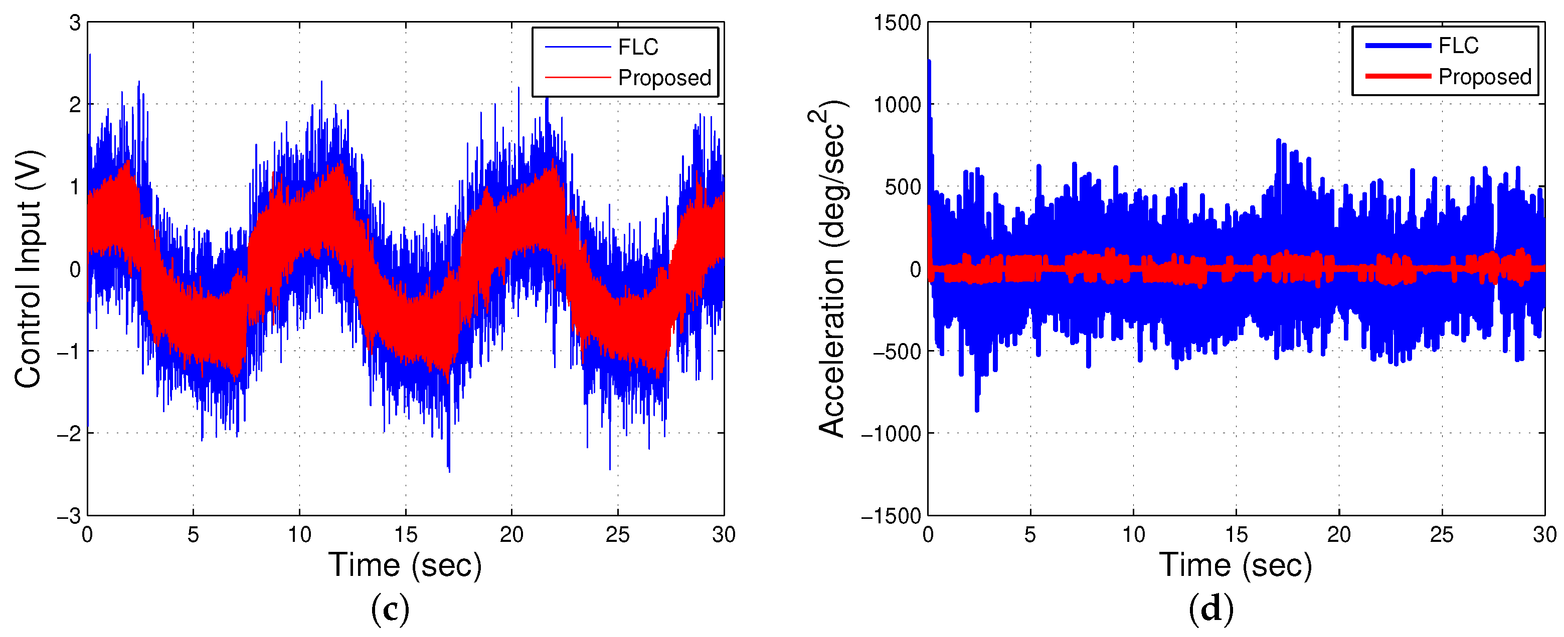
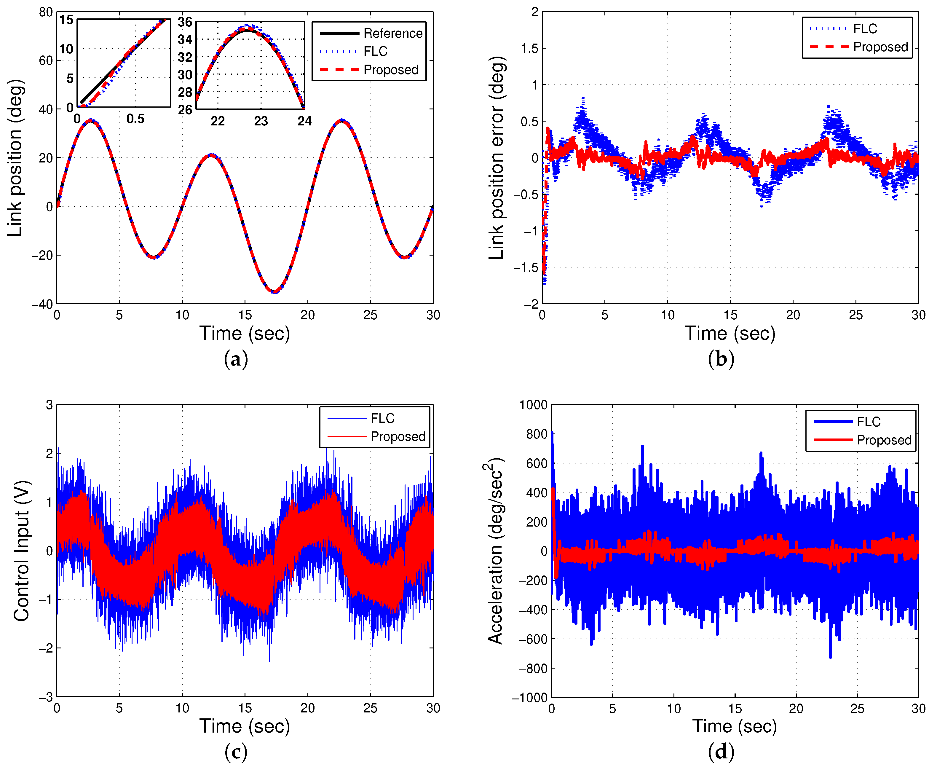
4.4.1. Sinewave Tracking Performance and Robustness (Tests 1 and 2)

In Test 1, the tracking trajectory efficiency of the FJR plant under no payload is tested. The desired reference command is a sinusoidal signal that is set by its amplitude and frequency of 35 deg and 0.1 Hz, respectively. The experimental results in Figure 9a–d demonstrate the angle of link position, the position error, estimated acceleration, and control input, respectively. As shown in Figure 9b, the proposed strategy achieves less tracking error than FLC. Furthermore, since the cascaded feature in the proposed observer construction is adopted, the noisy estimations are remarkably reduced and the chattering is well-reduced in the control signal, as clearly illustrated in Figure 9c,d, respectively.
To test the robustness of the proposed control against an uncertain payload, Test 2 is carried out by uploading an extra link to the original link payload. Figure 10a,b shows the angle of link position and the position tracking error, respectively. Figure 10a demonstrates that the proposed controller can closely track the desired reference even when the payload is present. The tracking error presented in Figure 10b is still smaller than the FLC approach in this test.

4.4.2. Dual Sine Waveform Tracking Performance and Robustness (Tests 3 and 4)

In both experiments 3 and 4, the trajectory tracking responses of the FJR are evaluated under a dual sinusoidal command. Here, the input reference is a combination of two sinusoidal signals determined by x d ( t ) = A 1 s i n ( 2 π F 1 t ) + A 2 s i n ( 2 π F 2 t ) , in which A 1 = 27 . 7 , A 2 = 10 , F 1 = 0.1 Hz and F 2 = 0.05 Hz, respectively. An inspection of Figure 11 demonstrates the practical results of experiment 3 in the absence of the payload effect, in which Figure 11a,b displays the link angular position and the tracking error, respectively. As can be shown from Figure 11, our designed control accomplishes a better performance, even in this different reference command, in contrast to the FLC approach.
Experiment 4 attaches an extra mass and increases the springs tension torque. Figure 12 illustrates the experimental results of Test 4, in which Figure 12a–d shows the position angle of the link, the tracking error, acceleration estimation, and the control signal, respectively. It is clearly found that the proposed controller causes little tracking error and fewer noises, even with the existence of the system uncertainties.

4.4.3. Sudden Load Compensation Capability (Test 5)

In this test, an external shock load disturbance is inserted to the control input channel in order to examine the efficacy of the proposed control in the existence of external disturbances. In the real situation, the sudden disturbance insertion emulates the robot arm that is attached to the drone, which could be impacted by an object, interact with a human, or be affected by a wind. As a result, those effects deflect the robot link from its zero equilibrium displacement. For this case, the control aim here is to enforce the link to return back to the equilibrium position as quickly and as precisely as possible. To carry out this case, we adjust the input reference to be zero, and then we apply two impulse voltages to the FJR plant at intervals of 5 s and 20 s, each having an amplitude of 1.5 V and a duration of 0.25 s. The angular position of the link illustrated in Figure 13 obviously shows that our designed controller fulfills a better anti-disturbance capability with a quick backdrivability of the link to the zero level, compared to the FLC method. Accordingly, the link part here can interact with this environmental situation freely.

4.5. Quantitative Comparison and Summary

To summarize the aforementioned experimental results, a quantitative analysis is performed by comparing the root mean square (RMS) values of the link tracking errors for the proposed controller and the FLC scheme, as shown in Table 1. It can be indicated that the proposed control approach attains a smaller RMS(e) in all aforementioned experiments, compared with the FLC approach.

5. Conclusions

This article has proposed a FxTSMC scheme based on a CFxTSMO for the underactuated aerial FJR manipulator fly arm attached to drones systems subjected to noise, uncertainties, and external disturbances. The mathematical model of the FJR with the underactuation has been transformed into the canonical representation via two transformations for the ease of the control design without the necessity of linearization and approximation. The main benefits of the proposed composite controller are that not only (i) can the parametric uncertainties, nonlinearities, and the external disturbances be estimated by the CFxTSMO estimator to relax the need for the uncertainty bound and to reduce the chattering by using a smaller switching gain, and (ii) the noise amplification in the states and disturbance estimations is remarkably minimized by employing the cascaded structure in the estimator design, resulting in the FxTSMC scheme being more feasible in practice for controlling the high-order FJR system, but also (iii) the fixed-time error convergence in the proposed CFxTSMO-based FxTSMC approach is well achieved, regardless of the unknown disturbance initial conditions. The extensive simulations and comparative experimental results for the actual FJR system have verified the superior performance and robustness of the proposed method. As a result, due to the ease of the practical implementation, this investigation suggests that our controller is a viable control option for other UMSs plants, such as drone systems.
Although the major limitation of the study is the measurement noise from the FJR system, according to the aforementioned benefits, this work brings significance for academics and practice to the control community by making the proposed control more feasible for high-order systems. In future work, we will experimentally test a fly robot mounted on drones under high frequencies of the reference trajectories by using the proposed control scheme.

Author Contributions

Conceptualization, K.R., Z.C. and Z.M.; methodology, K.R. and Z.C.; software, K.R.; validation, K.R. and Z.C.; formal analysis, K.R.; investigation, K.R., Z.C., L.W. and M.A.-R.; resources, Z.C., Z.M., L.W. and M.A.-R.; writing—original draft preparation, K.R.; writing— review and editing, Z.C., Z.M., L.W. and M.A.-R.; visualization, K.R., Z.C., Z.M., L.W. and M.A.-R.; supervision, Z.C. and Z.M.; project administration, Z.C.; funding acquisition, L.W. and M.A.-R. All authors have read and agreed to the published version of the manuscript.

Funding

This research was funded by the International Science and Technology Cooperation Project of the Shenzhen Science and Technology Commission (GJHZ20200731095804014).

Institutional Review Board Statement

Not applicable.

Informed Consent Statement

Not applicable.

Data Availability Statement

Not applicable.

Conflicts of Interest

The authors declare no conflict of interest.

References

  1. Ham, R.V.; Sugar, T.; Vanderborght, B.; Hollander, K.; Lefeber, D. Compliant actuator designs. IEEE Robot Autom Mag. 2009, 3, 81–94. [Google Scholar] [CrossRef]
  2. Talole, S.E.; Kolhe, J.P.; Phadke, S.B. Extended-state-observer-based control of flexible-joint system with experimental validation. IEEE Trans. Ind. Electron. 2010, 57, 1411–1419. [Google Scholar] [CrossRef]
  3. Le-Tien, L.; Albu-Schäffer, A. Robust Adaptive Tracking Control Based on State Feedback Controller with Integrator Terms for Elastic Joint Robots with Uncertain Parameters. IEEE Trans. Control Syst. Technol. 2018, 26, 2259–2267. [Google Scholar] [CrossRef]
  4. Sun, W.; Su, S.F.; Xia, J.; Nguyen, V.T. Adaptive Fuzzy Tracking Control of Flexible-Joint Robots with Full-State Constraints. IEEE Trans. Syst. Man Cybern. Syst. 2019, 49, 2201–2209. [Google Scholar] [CrossRef]
  5. Yunda, Y.; Zhang, C.; Narayan, A.; Yang, J.; Li, S.; Yu, H. Generalized Dynamic Predictive Control for Non-Parametric Uncertain Systems with Application to Series Elastic Actuators. IEEE Trans. Ind. Informat. 2018, 14, 4829–4840. [Google Scholar]
  6. Pan, Y.; Wang, H.; Li, X.; Yu, H. Adaptive command-filtered backstepping control of robot arms with compliant actuators. IEEE Trans. Control Syst. Technol. 2018, 26, 1149–1156. [Google Scholar] [CrossRef]
  7. Ginoya, D.; Shendge, P.; Phadke, S. Disturbance observer based sliding mode control of nonlinear mismatched uncertain systems. Commun. Nonlinear Sci. Numer Simulat. 2015, 26, 98–107. [Google Scholar] [CrossRef]
  8. Kim, J. Two-Time Scale Control of Flexible Joint Robots with an Improved Slow Model. IEEE Trans. Ind. Electron. 2018, 65, 3317–3325. [Google Scholar] [CrossRef]
  9. Pan, Y.; Li, X.; Yu, H. Efficient PID Tracking Control of Robotic Manipulators Driven by Compliant Actuators. IEEE Trans. Control Syst. Technol. 2019, 27, 915–922. [Google Scholar] [CrossRef]
  10. Rsetam, K.; Cao, Z.; Man, Z.; Mitrevska, M. Optimal second order integral sliding mode control for a flexible joint robot manipulator. In Proceedings of the 43rd Annual Conference of the IEEE Industrial Electronics Society, Beijing, China, 29 October–1 November 2017; pp. 3069–3074. [Google Scholar]
  11. Rsetam, K.; Cao, Z.; Man, Z. Hierarchical non-singular terminal sliding mode controller for a single link flexible joint robot manipulator. In Proceedings of the 56th Annual Conference on Decision and Control (CDC), Melbourne, Australia, 12–15 December 2017; pp. 6677–6682. [Google Scholar]
  12. Kim, J.; Croft, E.A. Full-state tracking control for flexible joint robots with singular perturbation techniques. IEEE Trans. Control Syst. Technol. 2019, 27, 63–73. [Google Scholar] [CrossRef]
  13. Qin, Z.C.; Xiong, F.R.; Ding, Q.; Hernández, C.; Fernandez, J.; Schütze, O.; Sun, J.Q. Multi-objective optimal design of sliding mode control with parallel simple cell mapping method. J. Vib. Control 2017, 23, 46–54. [Google Scholar] [CrossRef]
  14. Ginoya, D.; Shendge, P.; Phadke, S. Sliding mode control for mismatched uncertain systems using an extended disturbance observer. IEEE Trans. Ind. Electron. 2014, 61, 1983–1992. [Google Scholar] [CrossRef]
  15. Wang, H.; Pan, Y.; Li, S.; Yu, H. Robust Sliding Mode Control for Robots Driven by Compliant Actuators. IEEE Trans. Control Syst. Technol. 2019, 27, 1259–1266. [Google Scholar] [CrossRef]
  16. Haninger, K.; Tomizuka, M. Robust Passivity and Passivity Relaxation for Impedance Control of Flexible-Joint Robots with Inner-Loop Torque Control. IEEE/ASME Trans. Mechatron. 2018, 23, 2671–2680. [Google Scholar] [CrossRef]
  17. Jin, H.; Liu, Z.; Zhang, H.; Liu, Y.; Zhao, J. A Dynamic Parameter Identification Method for Flexible Joints Based on Adaptive Control. IEEE/ASME Trans. Mechatron. 2018, 23, 2896–2908. [Google Scholar] [CrossRef]
  18. Yan, Z.; Lai, X.; Meng, Q.; Wu, M. A novel robust control method for motion control of uncertain single-link flexible-joint manipulator. IEEE Trans. Syst. Man Cybern. Syst. 2019, 51, 1671–1678. [Google Scholar] [CrossRef]
  19. Rsetam, K.; Cao, Z.; Man, Z. Design of Robust Terminal Sliding Mode Control for Underactuated Flexible Joint Robot. IEEE Trans. Syst. Man Cybern. Syst. 2022, 52, 4272–4285. [Google Scholar] [CrossRef]
  20. Aghababa, M.P. Stabilization of canonical systems via adaptive chattering free sliding modes with no singularity problems. IEEE Trans. Syst. Man Cybern. Syst. 2018, 50, 1696–1703. [Google Scholar] [CrossRef]
  21. Rsetam, K.; Cao, Z.; Man, Z. Cascaded-extended-state-observer-based sliding-mode control for underactuated flexible joint robot. IEEE Trans. Ind. Electron. 2019, 67, 10822–10832. [Google Scholar] [CrossRef]
  22. Mishra, J.P.; Yu, X.; Jalili, M. Arbitrary-Order Continuous Finite-Time Sliding Mode Controller for Fixed-Time Convergence. IEEE Trans. Circuits Syst. II Exp. Briefs. 2018, 65, 1988–1992. [Google Scholar] [CrossRef]
  23. Song, J.; Hu, Y.; Su, J.; Zhao, M.; Ai, S. Fractional-Order Linear Active Disturbance Rejection Control Design and Optimization Based Improved Sparrow Search Algorithm for Quadrotor UAV with System Uncertainties and External Disturbance. Drones 2022, 6, 229. [Google Scholar] [CrossRef]
  24. Orozco Soto, S.M.; Cacace, J.; Ruggiero, F.; Lippiello, V. Active Disturbance Rejection Control for the Robust Flight of a Passively Tilted Hexarotor. Drones 2022, 6, 258. [Google Scholar] [CrossRef]
  25. Tian, B.; Lu, H.; Zuo, Z.; Zong, Q.; Zhang, Y. Multivariable finite-time output feedback trajectory tracking control of quadrotor helicopters. Int. J. Robust Nonlinear Control. 2018, 28, 281–295. [Google Scholar] [CrossRef]
  26. Basin, M.V.; Ramírez, P.C.R.; Guerra-Avellaneda, F. Continuous fixed-time controller design for mechatronic systems with incomplete measurements. IEEE/ASME Trans. Mechatron. 2017, 23, 57–67. [Google Scholar] [CrossRef]
  27. Tian, B.; Lu, H.; Zuo, Z.; Yang, W. Fixed-time leader–follower output feedback consensus for second-order multiagent systems. IEEE Trans. Cybern. 2018, 49, 1545–1550. [Google Scholar] [CrossRef] [PubMed]
  28. Basin, M.; Rodriguez-Ramirez, P.; Ding, S.X.; Daszenies, T.; Shtessel, Y. Continuous fixed-time convergent regulator for dynamic systems with unbounded disturbances. J. Frankl. Inst. 2018, 355, 2762–2778. [Google Scholar] [CrossRef]
  29. Zuo, Z.; Han, Q.L.; Ning, B. An Explicit Estimate for the Upper Bound of the Settling Time in Fixed-Time Leader-Following Consensus of High-Order Multivariable Multiagent Systems. IEEE Trans. Ind. Electron. 2018, 66, 6250–6259. [Google Scholar] [CrossRef]
  30. Basin, M.; Avellaneda, F.G. Continuous Fixed-Time Controller Design for Dynamic Systems with Unmeasurable States Subject to Unbounded Disturbances. Asian J. Control. 2019, 21, 194–207. [Google Scholar] [CrossRef] [Green Version]
  31. Olfati-Saber, R. Normal forms for underactuated mechanical systems with symmetry. IEEE Trans. Autom. Control. 2002, 47, 305–308. [Google Scholar] [CrossRef] [Green Version]
  32. Fliess, M.; Lévine, J.; Martin, P.; Rouchon, P. Flatness and defect of non-linear systems: Introductory theory and examples. Int. J. Control. 1995, 61, 1327–1361. [Google Scholar] [CrossRef] [Green Version]
  33. Angulo, M.T.; Moreno, J.A.; Fridman, L. Robust exact uniformly convergent arbitrary order differentiator. Automatica 2013, 49, 2489–2495. [Google Scholar] [CrossRef]
  34. Donaire, A.; Romero, J.G.; Ortega, R.; Siciliano, B.; Crespo, M. Robust IDA-PBC for underactuated mechanical systems subject to matched disturbances. Int. J. Robust Nonlinear Control. 2017, 27, 1000–1016. [Google Scholar] [CrossRef]
  35. Wu, X.; He, X. Nonlinear energy-based regulation control of three-dimensional overhead cranes. IEEE Trans. Autom. Sci. Eng. 2016, 14, 1297–1308. [Google Scholar] [CrossRef]
  36. Li, J.W. Robust Tracking Control and Stabilization of Underactuated Ships. Asian J. Control. 2018, 20, 2143–2153. [Google Scholar] [CrossRef]
  37. Sun, N.; Fang, Y.; Chen, H.; Wu, Y.; Lu, B. Nonlinear antiswing control of offshore cranes with unknown parameters and persistent ship-induced perturbations: Theoretical design and hardware experiments. IEEE Trans. Ind. Electron. 2017, 65, 2629–2641. [Google Scholar] [CrossRef]
  38. Sun, N.; Yang, T.; Fang, Y.; Lu, B.; Qian, Y. Nonlinear motion control of underactuated three-dimensional boom cranes with hardware experiments. IEEE Trans. Ind. Electron. 2017, 14, 887–897. [Google Scholar] [CrossRef]
  39. Dai, S.L.; He, S.; Lin, H. Transverse function control with prescribed performance guarantees for underactuated marine surface vehicles. Int. J. Robust Nonlinear Control. 2019, 29, 1577–1596. [Google Scholar] [CrossRef]
  40. Wang, X.; Liu, J.; Zhang, Y.; Shi, B.; Jiang, D.; Peng, H. A unified symplectic pseudospectral method for motion planning and tracking control of 3D underactuated overhead cranes. Int. J. Robust Nonlinear Control. 2019, 29, 2236–2253. [Google Scholar] [CrossRef]
  41. Zhang, A.; She, J.; Qiu, J.; Yang, C.; Alsaadi, F. Design of motion trajectory and tracking control for underactuated cart-pendulum system. Int. J. Robust Nonlinear Control. 2019, 29, 2458–2470. [Google Scholar] [CrossRef]
  42. Wu, Y.; Sun, N.; Fang, Y.; Liang, D. An increased nonlinear coupling motion controller for underactuated multi-TORA systems: Theoretical design and hardware experimentation. IEEE Trans. Syst. Man Cybern. Syst. 2017, 49, 1186–1193. [Google Scholar] [CrossRef]
  43. Bingol, O.; Guzey, H.M. Finite-Time Neuro-Sliding-Mode Controller Design for Quadrotor UAVs Carrying Suspended Payload. Drones 2022, 6, 311. [Google Scholar] [CrossRef]
  44. Shen, Z.; Tsuchiya, T. Singular Zone in Quadrotor Yaw–Position Feedback Linearization. Drones 2022, 6, 84. [Google Scholar] [CrossRef]
  45. Zuo, Z.; Han, Q.L.; Ning, B.; Ge, X.; Zhang, X.M. An overview of recent advances in fixed-time cooperative control of multiagent systems. IEEE Trans. Ind. Informat. 2018, 14, 2322–2334. [Google Scholar] [CrossRef]
Figure 1. Sketch of the FJR system attached to drone.
Drones 06 00428 g001
Figure 2. Block diagram of FxTSMC scheme with CFxTSMO estimator.
Drones 06 00428 g002
Figure 3. Flow chart and algorithm of proposed FxTSMC scheme with CFxTSMO estimator.
Drones 06 00428 g003
Figure 4. Time histories of link tracking errors with different initial conditions. (a) e 1 ( t ) ; (b) e 2 ( t ) ; (c) e 3 ( t ) ; (d) e 4 ( t ) .
Drones 06 00428 g004
Figure 5. Profiles of position tracking errors of link under different initial conditions. (a) x ( 0 ) = [ 10 0 , 0 , 0 , 0 ] T ; (b) x ( 0 ) = [ 20 0 , 0 , 0 , 0 ] T ; (c) x ( 0 ) = [ 30 0 , 0 , 0 , 0 ] T ; (d) x ( 0 ) = [ 40 0 , 0 , 0 , 0 ] T .
Drones 06 00428 g005
Figure 6. Profile of angular vibration of link under different initial conditions. (a) x ( 0 ) = [ 10 0 , 0 , 0 , 0 ] T ; (b) x ( 0 ) = [ 20 0 , 0 , 0 , 0 ] T ; (c) x ( 0 ) = [ 30 0 , 0 , 0 , 0 ] T ; (d) x ( 0 ) = [ 40 0 , 0 , 0 , 0 ] T .
Drones 06 00428 g006
Figure 7. Experimental platform of a Quanser FJR system.
Drones 06 00428 g007
Figure 8. Experimental module of a Quanser FJR system.
Drones 06 00428 g008
Figure 9. Experimental results with sinusoidal and no payload.
Drones 06 00428 g009aDrones 06 00428 g009b
Figure 10. Experimental results with sinusoidal and payload.
Drones 06 00428 g010
Figure 11. Experimental results with dual sinusoidal and no payload.
Drones 06 00428 g011
Figure 12. Experimental results with dual sinusoidal, and mass and spring changes.
Drones 06 00428 g012
Figure 13. Experimental results of the FJR, subject to shock disturbance.
Drones 06 00428 g013
Table 1. Performance Comparisons of Controllers in terms of RMS of tracking errors (deg).
MethodTest 1Test 2Test 3Test 4
Proposed0.07090.14140.11150.1453
FLC0.28780.37230.28350.3289
Improvement (%)75.46260.655.8
Publisher’s Note: MDPI stays neutral with regard to jurisdictional claims in published maps and institutional affiliations.

