Article

Computationally-Efficient Distributed Algorithms of Navigation of Teams of Autonomous UAVs for 3D Coverage and Flocking

School of Electrical Engineering and Telecommunications, The University of New South Wales, Sydney 2052, Australia
*
Author to whom correspondence should be addressed.
Drones 2021, 5(4), 124; https://doi.org/10.3390/drones5040124
Submission received: 22 September 2021 / Revised: 17 October 2021 / Accepted: 21 October 2021 / Published: 25 October 2021
(This article belongs to the Special Issue Conceptual Design, Modeling, and Control Strategies of Drones)

Abstract

:
This paper proposes novel distributed control methods to address coverage and flocking problems in three-dimensional (3D) environments using multiple unmanned aerial vehicles (UAVs). Two classes of coverage problems are considered in this work, namely barrier and sweep problems. Additionally, the approach is also applied to general 3D flocking problems for advanced swarm behavior. The proposed control strategies adopt a region-based control approach based on Voronoi partitions to ensure collision-free self-deployment and coordinated movement of all vehicles within a 3D region. It provides robustness for the multi-vehicle system against vehicles’ failure. It is also computationally-efficient to ensure scalability, and it handles obstacle avoidance on a higher level to avoid conflicts in control with the inter-vehicle collision avoidance objective. The problem formulation is rather general considering mobile robots navigating in 3D spaces, which makes the proposed approach applicable to different UAV types and autonomous underwater vehicles (AUVs). However, implementation details have also been shown considering quadrotor-type UAVs for an example application in precision agriculture. Validation of the proposed methods have been performed using several simulations considering different simulation platforms such as MATLAB and Gazebo. Software-in-the-loop simulations were carried out to asses the real-time computational performance of the methods showing the actual implementation with quadrotors using C++ and the Robot Operating System (ROS) framework. Good results were obtained validating the performance of the suggested methods for coverage and flocking scenarios in 3D using systems with different sizes up to 100 vehicles. Some scenarios considering obstacle avoidance and robustness against vehicles’ failure were also used.

1. Introduction

In recent years, there has been an increasing interest in mobile wireless sensor networks (MWSNs), where a number of networked autonomous vehicles can be deployed in different environments to achieve sensing tasks. Advances in communication made MWSNs more appealing where vehicles (sensors) can share information to perform cooperative monitoring, sensing, detection and exploration.
The problem of controlling multi-vehicle systems to achieve a global objective is referred to as cooperative control. There exist different subset problems related to this area depending on the common goal to be achieved by the vehicles. Coverage control deals with problems where a certain region of interest needs to be surveyed whether using a single vehicle or multiple (i.e., using MWSNs). Tackling these problems with multi-vehicle systems has given rise to new challenges to traditional cooperative control in the field of coverage control [1,2,3,4,5,6,7,8]. Unmanned aerial vehicles (UAVs) have become a popular choice in this area to form MWSNs especially in places inaccessible by ground vehicles. In general, multi-UAV systems have been emerging in various applications such as precision agriculture [9,10,11,12,13], aerial manipulation and transportation [14,15,16,17,18], search and rescue [14,19,20], firefighting [21], surveillance and monitoring [22,23], mapping and exploration [24,25,26], etc.
Coverage control problems can be classified as either static or dynamic. Another classification is based on [27] where coverage problems are categorized into Blanket coverage, Barrier coverage and Sweeping coverage, which are defined as follows:
  • Blanket coverage is forming a static arrangement to maximize the detection rate of events through an area of interest.
  • Barrier coverage is a static formation over some region (i.e., a barrier) to minimize intrusions or maximizing detection of objects going through it.
  • Sweeping coverage is the formation of dynamic arrangements moving across a region of interest for maximal detection/exploration along the whole region.
Clearly, blanket and barrier coverage problems belong to the static class while sweeping is a dynamic coverage problem.
Static coverage can be applied in different applications such as surveillance, real-time monitoring of crops, live stock and pollution, intruders detection in the security domain, etc. In these scenarios, the combined sensing field of view of all sensors is sufficient to monitor the regions of interest with a static configuration that the MWSN converges to. On the other hand, dynamic coverage is based on applications where the sensors need to remain mobile in order to survey the regions of interest. Examples of these applications include [28], but not limited to, autonomous search & rescue, monitoring of dynamically-changing environments, real-time monitoring of large areas with limited number of vehicles, visual inspection using multiple vehicles with limited combined field-of-view (FOV), firefighting in forests using a group of vehicles with limited spray area, autonomous irrigation with limited spray area, etc.
Flocking is another class of problems where cooperative control is applied, which is a subset of formation control, to deal with movement of large number of vehicles (swarms). In general, controlling a large number of vehicles to a achieve a common motion objective is motivated by collective behavior of animals such as bird flocks and fish schools. In this case, vehicles can make motion decisions by following a set of rules contributing towards the collective behavior (i.e., flocking). These rules are: flock centering (cohesion), collision avoidance (separation) and velocity matching (alignment) according to Reynold’s model [29,30].
The main contribution of this work is to develop novel distributed control strategies addressing cooperative control problems to achieve 3D coverage and flocking behavior. Specifically, the proposed methods address the 3D barrier and sweep coverage problems motivated by some of the ideas in [1,6,31]. In a 3D environment, a barrier can be defined as a static arrangement of sensors with overlapping sensing zones [32] forming a surface or a 3D region. The suggested control strategies rely on estimated centroidal Voronoi configurations over virtual regions generated by the sensors locations in a distributed manner depending only on shared information from neighbor vehicles. Furthermore, the suggested methods are also extended to address flocking problems in 3D spaces where the movement of the 3D virtual region is decided collectively by the group to achieve the common motion objective.
The designed control laws require relative distances with neighbor vehicles to be shared over communication channels which makes the overall problem related to Networked Control Systems (NCSs) [33,34,35,36,37,38,39]. The current work assumes that such information is available to the control system. However, several challenges related to communication channels imperfections needs to be considered when evaluating the performance of the overall networked control system. Thus, it is important to design a reliable communication system to allow for advanced swarming behaviors of robotic systems [40].
Overall, the vehicles’ collective motion becomes constrained within a specific dynamic region under the application of the suggested control methods similar to region-based shape control methods [41]. The dynamic region can be selected as a collection of non-overlapping polygons in 3D. Furthermore, one can control the dynamics of the dynamic region to generate 3D sweeping behavior which is the key idea used in the developed 3D sweeping coverage strategy. This is also considered to handle obstacle avoidance where vehicles can collaboratively control the dynamics of the virtual barrier and even apply deformations to its shape in real-time, which is then communicated through the networked multi-vehicle system. Furthermore, bounded control laws are proposed, which is important in practice to satisfy limits on the vehicles’ velocities and accelerations. The main advantages of the suggested approaches can be highlighted as follows:
  • collision avoidance among vehicles and connectivity is ensured by the adopted Voronoi-based approach
  • the approach is highly scalable and robust against vehicles’ failure
  • obstacle avoidance can be managed in a decomposed and distributed manner
A general 3D kinematic model is adopted in the design which is applicable to different UAV types and autonomous underwater vehicles (AUVs). A 6 degrees-of-freedom (DOF) dynamical model for quadrotors is further considered to show a possible way of implementation with low-level control design. Several simulations were carried out to validate the performance of the suggested methods in addition to showing its scalability and robustness. Moreover, software-in-the-loop (SITL) simulations were also performed using the Gazebo robotic simulator based on the quadrotor full dynamical model to evaluate the computational complexity of the implemented algorithms with particular interest in applications related to precision agriculture.
The organization of this paper is as follows. A summary of related works is given in Section 2 highlighting some of the drawbacks that motivated the proposed design. Section 3 introduces some essential concepts related to graph theory, locational optimization and Voronoi Partitions which are used in our control strategy, and the tackled 3D coverage problems are defined in Section 4. After that, distributed barrier and sweeping coverage control strategies are proposed in Section 5 considering a general 3D kinematic model. These approaches are validated through several simulation cases in Section 6. Furthermore, a generalization of the suggested methods is presented in Section 7 to address 3D flocking problems along with validation. Further implementation details considering quadrotors dynamics with low-level control design are presented in Section 8, which is evaluated using software-in-the-loop simulations. Finally, this work is concluded in Section 9 with a suggestion for a potential direction of future work.

2. Related Work

Coverage problems and optimal sensors deployment for both fixed and mobile wireless sensor networks have gained great interest over the years. According to [42], some of the common techniques used to address static coverage problems are resource-aware [43,44,45], search space-based [46,47], potential-based [48,49], Voronoi partition-based [1,5,31,50,51,52,53,54,55] and angle view [56,57,58].
An example algorithm of static deployment of cameras (i.e., non-mobile sensors) to achieve coverage with optimal resource allocation was proposed in [44]. In [43], modified Lloyd-like algorithms were developed to address the 2D static deployment of mobile sensors while considering optimizing the overall power consumption. The tradeoff between coverage performance and energy consumption of mobile heteregoneous wireless sensor networks was also investigated in [45].
Optimal placement of fixed and mobile networked sensors have been tackled in some works using optimization-based techniques. For example, the work in [46] adopted a particle swarm optimization-based approach to address the static deployment of cameras over 2D and 3D monitoring spaces for optimal visual monitoring. On the other hand, 2D static deployment of mobile wireless sensors was addressed in [47] using the Multi-objective Immune Algorithm (MIA). The problem formulation targeted the maximization of the coverage area while minimizing energy consumption due to movement. The authors have also considered the connectivity perseverance through limited movement within specified communication ranges. However, collision avoidance between mobile sensors and obstacles avoidance were not considered.
Another class of approaches addressing coverage problems of MWSNs is based on artifical potential field, which makes it easier to include collision avoidance rules as potential functions. In this case, control laws are designed based on gradient descent algorithms. For example, a decentralized approach was developed in [48] addressing the problem of deploying mobile sensors with limited sensing capeabilities to achieve the best possible coverage over an n-dimensional Euclideon space. The mobility of sensors was modeled as single integrator. The devleoped control law relies on forcing the inter-agent distances to reach a desired distance while avoiding collisions with other vehicles. Obstacle avoidance was not considered in this work. On the other hand, another method was presented in [49] using artificial potential fields considering both forces between the mobile sensors and obstacles in the environment to achieve both static deployment and collision avoidance. The method was validated considering only 2D environments.
A similar class of methods existing in the literature is based on Voronoi diagrams. The formulation of of such methods relies also on gradient descent algorithms adopting potential functions that can encode optimal coverage in a distributed manner, which was well developed in [1,31,59] with rigorous mathematical proofs. In these works, Lloyd’s algorithm was adopted to develop distributed control methods for motion coordination of MWSNs to achieve optimal coverage. Only 2D coverage problems were considered, and obstacle avoidance was not considered. The approaches were distributed in nature where each vehicle can compute its own Voronoi cell based on information shared from its Voronoi neighbours. Similarly, an adaptive 2D approach was proposed in [5] based on Voronoi diagrams. However, the authors of this work suggested a decentralized control law design, where each vehicle can approximate the centroid of its Voronoi cell based only on its sensory measurements rather than relying on information received from its Voronoi neighbors. This can be more practical in cases where Voronoi neighbors are at distances larger than the vehicle’s communication range. This approach was also considered in [50]; however, a different weighting function, which defines the sensing performance over a planar region, was considered.
Many of the above approaches consider planar circular sensing models. Some works have considered different sensing models such as [51,52]. In these works, non-uniform unequally scaled 2D sensing footprints were considered. Additionally, Voronoi partitioning was performed only with respect to the sensed space, rather than the whole region of interest as in the previous methods.
Some research works have also considered additional requirements in the coverage problem formulation such as graph connectivity perseverance and information routing. For example, the 2D static coverage problem tackled in [53] considered that the mobile sensors are required to send the collected sensory information to a set of destinations over the network while performing the coverage task. Their solution was based on a constrained optimization problem considering Voronoi partitioning as part of the solution.
The above methods are mainly developed to address static coverage problems of MWSNs, where the sensors need to converge to a static arrangement with optimal coverage. There also exist methods addressing dynamic coverage problems such as [28,60,61,62,63,64,65,66]. In [28], a multi-agent system was considered with a 2D nonholonomic agent model. The approach relied on a leader-follower paradigm, where the vehicles try to maintain desired distances from a position targeted by the leader. This can be more challenging in 3D and for systems with large number of vehicles. Another approaches considering 2D nonhonolomic agents were developed in [61,62] proposing control laws based on a special form of Lyapunov-like functions to achieve satisfactory coverage level and collision avoidance.
Motivated by the Voronoi-based static coverage methods, the work in [63] suggested a planar approach based on modified Voronoi partitions with time-varying density functions, which describe the coverage performance, to address the planar dynamic coverage problem. However, obstacle avoidance was not considered in this work. A similar approach was also proposed in [63] where the authors suggested a Bayesian prediction method to estimate the unknown time-varying density function.
Overall, many of the existing static and dynamic coverage control approaches consider only two-dimensional sensing fields, and the literature lacks a proper analysis of sensor networks deployed in three-dimensional (3D) sensing fields [67]. Even those methods proposed for multi-UAV and multi-AUV systems assume that the vehicles are moving at a fixed altitude/depth with a planar sensing footprint without utilizing the full capabilities of such vehicles. It is hence more motivating to work towards addressing 3D coverage problems exploiting the rich geometric properties of 3D MWSNs [67]. Some efforts have been made in that area such as [32,67,68,69,70,71,72,73]. Thus, one of the main motivations of this work is to contribute towards the state-of-the-art 3D static and coverage problems using MWSNs.
On the other hand, the flocking problem has also attracted great interest. Many researchers have tackled the flocking control problem where the global group objective is to move the whole group towards some goal region or to follow a certain motion pattern (for example, see [29,74,75,76,77,78,79,80,81,82,83]). Most of state-of-the-art flocking control methods rely completely on artificial potential field to handle local interactions between vehicles, which have some disadvantages such as being prone to getting stuck at a local minimum especially due to conflicts between forces required to achieve moving towards goal, collision avoidance and obstacle avoidance control objectives. To address these limitations, the suggested control strategy separates the control components for these objectives on different layers as will be shown later.

3. Preliminaries

The proposed methods in paper relies on concepts from graph theory, locational optimization and Voronoi partitions. A summary of these concepts is provided in this section based on [1,29,31,59]. Note that when considering a multi-UAV system as a mobile wireless sensor network, UAVs may interchangeably referred to throughout the paper as sensors, nodes, agents or vehicles.

3.1. Graph Theory

A multi-UAV sensor network consisting of n UAVs can generally be characterized using a set of nodes/vertices U = { 1 , 2 , , n } and a set of edges (paired vertices) E { ( i , j ) : i , j U , j i } . Note that i and j will be used in the rest of the paper to refer to the index of a node/vertex within a set (i.e., index of a UAV within the group). Each vertex corresponds to a single UAV/sensor, and edges represent interaction between UAVs which are within communication or detection range from each others. The overall network topology is then described using a graph G = ( U , E ) which can be directed or undirected. In an undirected graph, an edge exists from vertex i to vertex j if and only if an edge exists from j to i (i.e., ( i , j ) E ( j , i ) E ). Otherwise, the graph is called directed. Generally, homogeneous multi-UAV systems can be described using undirected graphs since all UAVs have same communication and sensing capabilities. Moreover, a path between two vertices i 0 and i k is defined as a sequence of vertices { i 0 , i 1 , , i k } U where an edge exists between each subsequent vertices in the sequence such that ( i l , i l + 1 ) E , l { 0 , 1 , , k 1 } . If every pair of vertices in U is connected by a path, the graph G ( U , E ) is then called connected. Clearly, a crucial part for MWSNs is to maintain network connectivity all the time.
Furthermore, define a neighborhood  N i around a vertex i as the set of all vertices which have edges with vertex i such that:
N i = { j U \ { i } : ( i , j ) E } .
For a homogeneous system, let r > 0 denote the communication range for all UAVs. Hence, all UAVs within a spherical region of radius r around UAV i belong to its neighborhood such that
N i = { j U \ { i } : | | p i p j | | r } ,
where p i I R 3 is the position of UAV i, and | | · | | is the Euclidean norm in I R 3 . Similarly, all norms in the rest of the paper are Euclidean norms in I R 3 .

3.2. Locational Optimization

Deployment of mobile sensors in an environment to achieve optimal sensor coverage is regarded as a multicenter problem from locational optimization (i.e., spatial resource-allocation problem). A brief description about some of the facts related to this class of problems is summarized next based on [1,59].
Consider a bounded region of interest Q , including its interior, defined in a space I R d with dimension d. A partition of Q consists of a group of n non-overlapping polytopes W = { W 1 , , W n } such that W 1 W n = Q . Furthermore, let ϕ : Q I R + , ( I R + = { a I R : a > 0 } ) be defined as a distribution density function representing a measure of information or the likelihood of an event to take place over Q . The sensing performance of a sensor located at some position p i as seen from any point q Q depends mostly on the distance | | q p i | | . Clearly, as this distance increases, the sensing performance degrades. Hence, one can describe the sensing performance at location q of the sensor p i using a non-increasing piecewise continuously differentiable function f ( | | q p i | | ) : I R + I R . Thus, the larger the value of f, the better the sensing performance at q is.
Using the above definitions, one can define a multicenter cost function characterizing the average coverage provided by a set of n sensors at p 1 , , p n over an point in Q as follows:
H ( p 1 , , p n ) = Q max i { 1 , , n } f ( | | q p i | | ) ϕ ( q ) d q .
The above function provides a measure of the sensing performance expected value provided by all sensors at any point q Q [31]. Now, in order to find the optimal placement for all sensors, an optimization problem needs to be solved to maximize the value of H ( p 1 , , p n ) .
Remark 1.
Note that there are slightly different definitions for f in the references [1,31,59] where it can be either considered as a representation of sensing degradation or sensing performance over Q (as considered here). This does not affect the overall analysis done here except that the considered optimization problem will either be minimization (of sensing degradation) or maximization (of sensing performance).

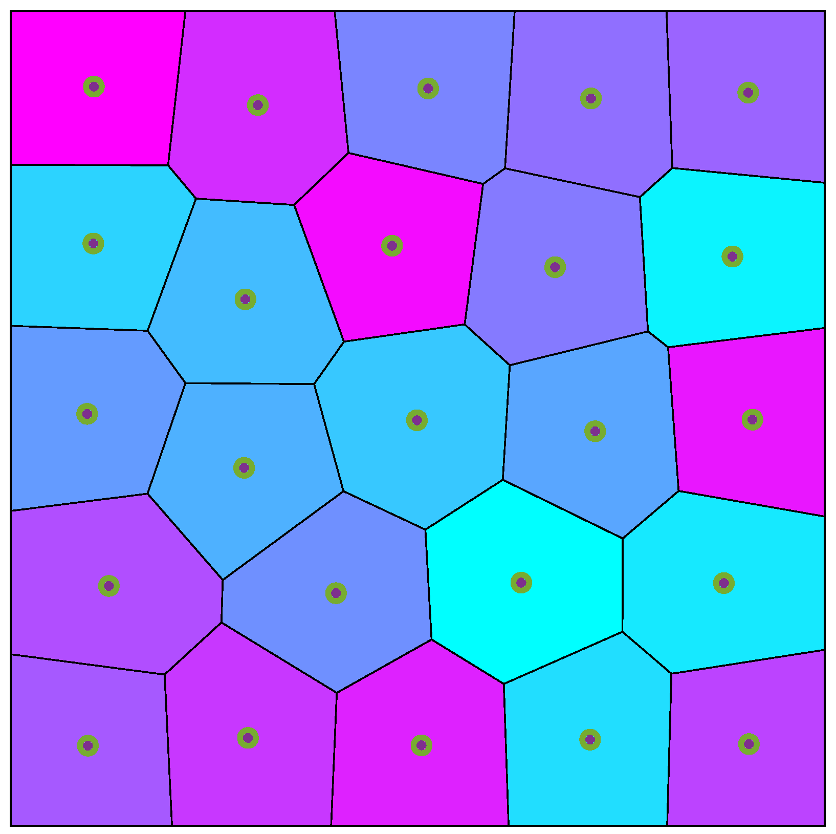
3.3. Voronoi Partitions (Tessellation)

This subsection highlights some key points about Voronoi partitions needed for our problem formulation. A Voronoi partition/tessellation is the subdivision of a space into a number of regions generated by a set of points (see Figure 1 for a 2D example). Consider that we have n sensors located at fixed locations P = { p 1 , , p n } Q n . A voronoi partition of Q consists of a set of disjoint Voronoi regions/cells V ( P ) = { V 1 , , V n } generated by these sensors where
V i = { q Q : | | q p i | | | | q p j | | , j i } ,
and V 1 V 2 V n = Q .
It has been established that this Voronoi partition is the optimal partition of Q among all other partitions [59]. For any sensor located at a position p i , its Voronoi neighbors N V , i P are defined as the sensors corresponding to adjacent Voronoi cells such that:
N V , i = { j { 1 , , n } : V i V j , j i } .
Considering the above definition, one can rewrite (3) as:
H V ( P , V ( P ) ) = i = 1 n V i ( P ) f ( | | q p i | | ) ϕ ( q ) d q .
By taking the partial derivative of (6) with respect to p i , the following is obtained:
H V p i ( P , V ( P ) ) = V i p i f ( | | q p i | | ) ϕ ( q ) d q ,
where it is assumed that f does not have any discontinuities. Furthermore, considering f ( x ) = x 2 , the multicenter cost function in (6) becomes:
H V ( P , V ( P ) ) = i = 1 n V i ( P ) | | q p i | | 2 ϕ ( q ) d q : = i = 1 n J V i , p i ,
where J V i , p i is the polar moment of inertia of V i about p i . Consequently, (8) reduces to:
H V p i = 2 M V i ( C V i p i ) ,
where M V i I R + and C V i I R 3 are the mass and center of mass (centroid) of the corresponding Voronoi partition V i with respect to the density function ϕ ( q ) . It is clear from (9) that the critical points of H V ( P , V ( P ) ) are the configurations P Q n where p i = C V i i , which are referred to as centroidal Voronoi configurations.

4. 3D Coverage Problems

Consider a 3D bounded region of interest S I R 3 . A multi-vehicle system can perform coverage tasks over S where coverage objective may vary according to the problem in hand. Definitions of the considered barrier and sweep coverage problems in 3D are defined next.
Problem 1.
(3D Barrier Coverage) Deploy a network of vehicles/sensors to form a static arrangement over some region B S (i.e., a barrier) maximizing the sensing performance of the overall network to detect any intruder going through the barrier.
A special case of the above problem is when deploying the sensors over a planar region within S defined by B = { ( x , y , z ) : σ ( x , y , z ) = 0 } where σ ( x , y , z ) is the plane’s equation. Note that for this problem to be solvable, the number of vehicles/sensors needed depends on the size of S and the sensing range of all vehicles (assuming a homogeneous system).
Problem 2.
(3D Sweep Coverage) Consider a group of vehicles whose overall sensing range is not large enough to achieve complete coverage over S . It is required to survey the region S by moving the whole group across S as a dynamic formation over some region F ( t ) S .
The coverage task can be considered completed once the whole region S is scanned/surveyed. Alternatively, the coverage task can be done repetitively over a specified period of time (i.e., continuously survey S for several times).
Note that F ( t ) can be of any 3D shape in which its motion along S following a certain pattern can achieve complete coverage. A special case is when F ( t ) is a plane which is considered in this work. In this case, F ( t ) will referred to as the sweeping plane. The dynamics of the sweeping plane F ˙ ( t ) can be determined in a way to achieve complete coverage over S . It is also assumed that F ( t ) can change size and shape over time which can be utilized for other motion objectives such as obstacle avoidance as will be shown later.

Problem Formulation

The aim of this work is to develop distributed control laws for multi-UAV systems to address Problems 1 and 2. We consider a system of n homogeneous vehicles (UAVs/AUVs) with a single integrator motion model given by:
p ˙ i ( t ) = u i ( t ) ,
where p i I R 3 is the i-th vehicle position defined in some inertial frame { I } , and u i I R 3 is its control input (velocity) where
u i u m a x .
All vehicles can sense events in the environment within a sensing range r s > 0 . Furthermore, any vehicle can exchange information with nearby vehicles within some communication range r c > 0 . Obviously, it is assumed that r c > r s so that it is possible to design control laws which can maintain the connectivity of the network with minimal sensors overlapping. It is assumed that the vehicles are homogeous in terms of sensing and communication ranges. However, they can be of different types, sizes and/or weights.

5. Distributed Coverage Control Strategies

The proposed control schemes to address Problems 1 and 2 are based on a self-deployment method for the multi-vehicle system over a planar region B S which is static for barrier coverage problems and dynamic for sweep coverage problems. We consider a set of l vertices E to describe the boundary of B as a polygon such that E = { e 1 , e 2 , , e l } S ; clearly, l > 2 . Lloyd’s algorithm is adopted in the designed controllers to guide the vehicles to reach the instantaneous centroids of their associated Voronoi regions over B (i.e., reaching the centroidal Voronoi configuration). Once this is reached, an optimal coverage over B is achieved. Furthermore, for sweeping problems, the designed dynamics of B will achieve coverage over S .

5.1. Online Computation of Centroidal Voronoi Configurations

The developed control law requires each vehicle to be able to compute the centroid of its Voronoi region in a distributed fashion based only on information exchanged with vehicles within its neighbourhood. We extend the approach proposed in [1] to compute Voronoi cells for planar regions in 3D in a distributed fashion.
To simplify the mathematical development, a new 3D coordinate frame { B } attached to B is needed. The origin of { B } can be selected to be one of the barrier vertices defined as O B = e 1 . Furthermore, the axes of { B } are defined using the orthonormal basis { a 1 , a 2 , a 3 } where:
a 1 = e 2 e 1 | | e 2 e 1 | | a 2 = h ( a 1 , b ) | | h ( a 1 , b ) | | , b = e l e 1 | | e l e 1 | | a 3 = a 1 × a 2 ,
where h ( w 1 , w 2 ) = w 2 ( w 1 · w 2 ) w 1 is a mapping function which gives an orthogonal vector to w 1 I R 3 directed towards w 2 I R 3 .
All computations needed to find Voronoi centroids are carried out in the { B } frame through a transformation between { B } and the inertial frame { I } . Let v I I R 3 be a vector defined in the { I } frame. This vector can be transformed to the { B } coordinate frame using a transformation matrix T I B as follows:
v B 1 = T I B v I 1 ,
where T I B is a 4 × 4 affine transformation matrix given by:
T I B = T B I 1 = a 1 a 2 a 3 O B 0 0 0 1 1 .
Note that we represent the transformation using an augmented matrix to consider both rotation and translation in a single matrix multiplication. Furthermore, a 1 , a 2 , a 3 , and O B are column vectors.
From now on, vectors represented in the inertial frame will be represented without the I superscript for simplicity. Given a UAV at position p i , it is required to compute instantaneous Voronoi centroid C V i of its projection onto B . First, the following assumption is made.
Assumption 1.
Each Voronoi cell V i B , generated by the projection of UAV i onto B , is a convex polygon defined by m vertices { v 1 B , v 2 B , , v m B } where v j B = ( x ¯ j , y ¯ j , 0 ) , j = { 1 , , m } .
The proposed approach can now be described in these steps:
S1:
Transform the position p i into the { B } frame to obtain p i B = [ x ¯ i , y ¯ i , z ¯ i ] T by applying (13).
S2:
Compute the projection of p i B onto B defined in the { B } frame by setting z ¯ i = 0 as p ˜ i B = [ x ¯ i , y ¯ i , 0 ] T .
S3:
Compute the Voronoi cell centroid C ˜ V i B = [ c ¯ x , V i , c ¯ y , V i , 0 ] T associated with p ˜ i B using the following [1]:
M V i = 1 2 k = 1 m ( x ¯ k y ¯ k + 1 x ¯ k + 1 y ¯ k ) c ¯ x , V i = 1 6 M V i k = 1 m ( x ¯ k + x ¯ k + 1 ) ( x ¯ k y ¯ k + 1 x ¯ k + 1 y ¯ k ) c ¯ y , V i = 1 6 M V i k = 1 m ( y ¯ k + y ¯ k + 1 ) ( x ¯ k y ¯ k + 1 x ¯ k + 1 y ¯ k ) ,
where v m + 1 B = ( x ¯ m + 1 , y ¯ m + 1 , 0 ) = v 1 B . These equations are obtained considering Assumption 1 and a constant distribution density function ϕ ( q ) = 1 . Voronoi cell vertices { v 1 B , v 2 B , , v m B } can be determined based on locations of Voronoi neighbours in a distributed fashion (see Remark 2).
S4:
Transform C ˜ V i B to the inertial frame { I } to get C ˜ V i = [ c x , V i , c y , V i , c z , V i ] T using (13).
Remark 2.
The vertices of a Voronoi cell V i can be found as the circumcenters of triangles formed by p ˜ i B and any two of its Voronoi neighbours. A triangle made by three points p 1 , p 2 and p 3 with an area of A has a circumcenter at [1]:
c i r c u m c e n t e r = 1 4 A ( | | α 32 | | 2 ( α 21 · α 13 ) p 1 + | | α 13 | | 2 ( α 32 · α 21 ) p 2 + | | α 21 | | 2 ( α 13 · α 32 ) p 3 ) ,
where α l s = p l p s .

5.2. Barrier Coverage Control Design

In order to present our control design, some technical assumptions need to be made as follows.
Assumption 2.
The communication graph G ( U , E ) remains connected for t 0 .
Assumption 3.
Each UAV is capable of estimating the Voronoi cell centroid of its projected position onto B at any time using only information from UAVs within its communication range (i.e., UAVs in its neighborhood N i ).
Assumption 4.
The Voronoi neighbours of p ˜ i B correspond to UAVs within the neighbourhood N i .
Assumption 5.
The initial configuration of the multi-UAV system satisfies the following condition: p i ( 0 ) p j ( 0 ) | | p i ( 0 ) p j ( 0 ) | | · a 3 ± 1 , i , j { 1 , , n } , i j where a 3 is the barriers normal as defined in (12).
Assumption 2 is made to make sure that updated information about the barrier B is available to all vehicles at any time during the motion. This is essential in cases where B is dynamic. For example, a decision could be made by one of the UAVs to apply changes to the shape of B based on some detected obstacles. Such information needs to be shared among all vehicles so that they can compute their Voronoi regions accordingly. It is possible to ensure the connectivity of G ( U , E ) by enforcing constraints on B based on the number of vehicles and communication ranges to ensure that Voronoi neighbors are within the communication range of each others. Assumptions 3 and 4 ensures that UAVs can determine Voronoi centroids in a distributed fashion. Finally, Assumption 5 ensures that all UAVs are initially located at positions with unique projections onto B .
Now, the main results of this section can be presented. Consider the following control law u i : I R 3 I R 3 based on Lloyd’s algorithm:
u i = K ¯ i ( C ˜ V i p i ) ,
where the parameter K ¯ i is a diagonal positive definite gain matrix. We also propose a more practical bounded control law u i : I R 3 Γ which can satisfy bounds u m a x on the control input such that Γ = { u I R 3 : | | u | | u m a x } . It is given as follows:
u i = K i tanh γ i ( C ˜ V i p i ) ,
where K i = d i a g { k i , x , k i , y , k i , z } is a positive definite diagonal matrix, γ i > 0 , and tanh ( v ) is the hyperbolic tangent function defined element-wise for any vector v I R 3 . Clear, the bound of this control law depends on the gain matrix K i as follows:
| | u i | | k i , x 2 + k i , y 2 + k i , z 2 : = u i , m a x .
Theorem 1.
Consider a multi-UAV system with n vehicles whose motion are modelled as (10). Under Assumptions 2–5, the distributed control law (16) (or (17) for bounded inputs) along with the algorithm inS1-S4solves the 3D barrier coverage problem defined in Problem 1.
Proof. 
Let P e be a centroidal Voronoi configuration. We define a Lyapunov canidate function as
V 1 ( P ( t ) ) = 1 2 H ¯ 1 2 H V ( P ( t ) , V ( P ( t ) ) ) ,
where H V is defined in (8) with ϕ ( q ) = 1 , and H ¯ = H V ( P e , V ( P e ) ) which is constant. Hence, V 1 ( P e ) = 0 . Furthermore, H ¯ H V ( P ( t ) , V ( P ( t ) ) ) P S n \ { P e } since a centroidal Voronoi configuration is optimal for H V among all other configurations (see Proposition 2.14 in [59]). This indicates that V 1 ( P ( t ) ) > 0 which makes it a valid Lyapunov function.
The time derivative of (19) can be obtained using (9) and (10) and the control law (16) as:
V ˙ 1 = 1 2 i = 1 n H V p i T u i
= i = 1 n ( C ˜ V i p i ) T L ¯ i ( C ˜ V i p i )
i = 1 n λ m i n ( L ¯ i ) C ˜ V i p i 2 ,
where L ¯ i = M V i K ¯ i , and λ m i n ( L ¯ i ) is the smallest eigenvalue of L ¯ i . It is clear from (22) that V ˙ 1 < 0 P S n \ { P e } since K ¯ i is positive definite (i.e., λ m i n ( L ¯ i ) > 0 ). Hence, the set of centroidal Voronoi configurations P e is locally asymptotically stable, and lim t p i = C ˜ V i , i .
Similarly, for the bounded control law, the time derivative of V 1 ( P ( t ) ) can be obtained by substituting (17) into (20) as follows:
V ˙ 1 = i = 1 n ( C ˜ V i p i ) T L i tanh γ i ( C ˜ V i p i )
: = i = 1 n e i T L i tanh ( γ i e i ) .
It is evident from (24) that V ˙ 1 < 0 P S n \ { P e } since the hyperbolic tangent function is an odd function and γ i > 0 . This implies that P e is also locally asymptotically stable under the application of the bounded control law (17).
Therefore, the control law (16) (or (17)) guarantees that the vehicles will converge to centroidal Voronoi configurations which maximizes the sensing performance over the barrier B according to Proposition 2.13 in [59]. Furthermore, Assumptions 2–5 ensures that all vehicles can compute the centroids of their Voronoi cells in a distributed fashion at all times with no overlapping following the algorithm in S1S4. This completes the proof. □
Note that the proposed control law ensures that the vehicles will converge to centroidal Voronoi configurations generated by their projections onto B . Thus, all the vehicles will eventually reach B such that lim t p i = C ˜ V i B even if they are initially deployed at some positions p i ( 0 ) B . Additionally, the trajectory of each vehicle remains within its Voronoi region which does not intersect with any other regions by definition. This guarantees that vehicles motions are collision-free using the proposed control laws.

5.3. Sweep Coverage Control Design

Theorem 1 shows that the proposed control laws can force the vehicles to reach a specified region within the 3D space (i.e., the barrier) and constrain their motion within that region. This is extended in this section to address the sweep coverage control problems. It can be achieved by enforcing vehicles to deploy over some dynamical "virtual" region whose motion is determined by the group.
In general, motion coordination control laws for coverage problems needs to satisfy the following objectives:
O 1
 Avoid collisions with other vehicles while maintaining a certain formation as a group
O 2
 Avoid collisions with obstacles within the environment
O 3
 Achieve optimal coverage of the targeted environment S collaboratively
The proposed sweeping algorithm targets these objective on two levels. At a lower level, the vehicles motions are constrained within a dynamic “sweeping” region F ( t ) S , and they maintain an optimal formation over that region for maximal sensing. This achieves objective O 1 . At a higher level, decisions can be made in real-time collaboratively by the vehicles to decide the dynamics of F ( t ) (i.e., F ˙ ( t ) ). Note that it is also possible to apply deformations to F ( t ) (will be shown in simulations) as long as the deformed region is large enough for the vehicles to distribute over with safe spacing. This provides a good way in addressing objectives O 2 and O 3 . In particular, the trajectory of F ( t ) will result in sweeping the whole environment S providing optimal coverage. Moreover, obstacle avoidance can be achieved by only changing the dynamics of F ( t ) rather than having each vehicle reacting independently to obstacles.
For r F ( t ) , the motion dynamics of the sweeping region can be described as follows:
r ˙ = g ( t , r ) , g ( t , r ) g ¯ , g ˙ ( t , r ) g ¯ ¯ ,
where g ( t , r ) I R 3 is a desired velocity profile, g ¯ , g ¯ ¯ > 0 are upper bound design parameters to account for dynamic limitations where the following condition must hold:
g ¯ u m a x .
In other words, the speed of F ( t ) should not be larger than the maximum physical speed that can be achieved by the vehicles. Note that g ( t , r ) I R 3 can have any direction. However, for simplicity in achieving sweeping coverage, it assumed that F ( t ) is a planar region, and it is defined similar to B (see Section 5.1) at different time instants. A simple example is moving F ( t ) in the direction of its normal (i.e., a 3 ) with a constant sweeping speed g 0 > 0 such that:
g ( t , r ) = g 0 a 3 .
More complex movements can be achieved depending on the considered environment shape and nearby obstacles. One can also adopt a 3D holonomic or non-holonomic model for (25) utilizing the available literature in obstacle for these models. Generally, obstacle avoidance can be achieved either by varying the dynamics in (25) or by dynamically deforming F ( t ) . Simulation cases showing both approaches will be shown later. Note that the distributed behavior of the proposed algorithm is maintained in all these cases since information about g ( t , r ) are exchanged over the connected network following Assumption 2. At this point, we will leave out the design of (25) to a high-level controller shared among the vehicles while assuming the following:
Assumption 6.
The sweeping plane F ( t ) remains all the time within the sensing environment (i.e., F ( t ) S , t > 0 ), and its movement governed by (25) will completely span the volume of the sensing environment S .
The main results of this section can now be presented.
Theorem 2.
Consider a multi-UAV system of size n where each vehicle’s motion model is represented by (10). The control law (16) along with the algorithm in S1S4 defined for a sweeping region F ( t ) whose dynamics is governed by (25) solves the 3D sweeping coverage problem defined in Problem 2 under Assumptions 2–6 and the condition (26).
Proof. 
Let
e C i = C ˜ V i p i e ˙ C i = C ˜ ˙ V i u i ,
where u i ( t ) is given by (16). Now, define a Lyapunov candidate function as follows:
V 2 ( t ) : = V 2 ( e C 1 ( t ) , , e C n ( t ) , e ˙ C 1 ( t ) , , e ˙ C n ( t ) ) = V 1 + 1 2 i = 1 n k 1 e C i T e C i + k 2 e ˙ C i T e ˙ C i ,
where V 1 is defined in (19), and k 1 and k 2 are positive kinematic constants with units of m 2 and m 2 · s 2 to match the physical units of V 1 which is m 4 . The choice (29) guarantees that V 2 ( t ) > 0 for
( e C 1 ( t ) , , e C n ( t ) , e ˙ C 1 ( t ) , , e ˙ C n ( t ) ) ( 0 , , 0 ) ,
and V 2 ( 0 , , 0 ) = 0 is also true.
The time derivative of (29) is obtained using (10) and (16) as follows:
V ˙ 2 = V ˙ 1 + i = 1 n k 1 e C i T e ˙ C i + k 2 e ˙ C i T e ¨ C i = V ˙ 1 + i = 1 n k 1 e C i T ( C ˜ ˙ V i K ¯ i e C i ) + k 2 e ˙ C i T ( C ˜ ¨ V i K ¯ i e ˙ C i ) V ˙ 1 + i = 1 n k 1 C ˜ ˙ V i e C i λ m i n ( K ¯ i ) k 1 e C i 2 + g ¯ ¯ k 2 e ˙ C i λ m i n ( K ¯ i ) k 2 e ˙ C i 2
Recall that V ˙ 1 < 0 which was established in (24). Therefore, the time derivative of V 2 is negative outside the compact set B Γ = B Γ 1 B Γ n where B Γ i = { e C i I R 3 , e ˙ C i I R 3 : e C i > Γ i , 1 , e ˙ C i > Γ i , 2 } and Γ i , 1 and Γ i , 2 are given by:
Γ i , 1 = C ˜ ˙ V i λ m i n ( K ¯ i ) , Γ i , 2 = g ¯ ¯ λ m i n ( K ¯ i ) ,
which represent closed balls with radius Γ i , 1 and Γ i , 2 respectively. Thus, starting from any initial condition outside the set B Γ , the errors will converge to the closed set B Γ in finite time and stay there forever. That is,
lim sup t C ˜ V i p i Γ i , 1 , lim sup t C ˜ ˙ V i u i Γ i , 2 ,
which means that the errors will be uniformly ultimately bounded with respect to B Γ i . Moreover, the radius of B Γ i can be made arbitrary small by increasing K ¯ i such that λ m i n ( K ¯ i ) g ¯ and λ m i n ( K ¯ i ) g ¯ ¯ . Furthermore, since C ˜ V i F ( t ) , its derivative follows (25) (i.e., lim sup t g ( t , C ˜ V i ) u i Γ i , 2 ). Hence, all the vehicles will converge to their centroidal Voronoi configurations over F ( t ) and follow its trajectory associated with (25). According to Assumption 6, the movement of the multi-UAV along the trajectory of F ( t ) solves the sweeping coverage problem. This completes the proof. □
Theorem 3.
Consider a multi-UAV system of size n where each vehicle’s motion model is represented by (10). Furthermore, consider using the algorithm inS1S4defined for a sweeping region F ( t ) whose dynamics is governed by (25) so that the vehicles can compute their centroidal Voronoi configurations. The bounded control law (17) solves the 3D sweeping coverage problem defined in Problem 2 under Assumptions 2–6 and the condition (26).
Proof. 
Again, consider the errors definitions in (28). We now define a Lyapunov candidate function as follows:
V 3 ( t ) : = V 3 ( e C 1 ( t ) , , e C n ( t ) , e ˙ C 1 ( t ) , , e ˙ C n ( t ) ) = V 1 + i = 1 n k 3 γ i [ 1 1 1 ] T log ( cosh ( γ i e C i ) ) + 1 2 k 4 e ˙ C i T e ˙ C i ,
where log ( v ) I R 3 and cosh ( v ) I R 3 are defined element-wise for any vector v I R 3 , k 3 and k 4 are positive kinematic constants, and u i is defined using (17). Furthermore, let S e c h 2 ( v ) : I R 3 I R 3 × 3 be a mapping function, based on the hyperbolic secant function, which maps the vector v = [ v 1 , v 2 , v 3 ] T into a diagonal matrix as follows:
S e c h 2 ( v ) = s e c h 2 ( v 1 ) 0 0 0 s e c h 2 ( v 2 ) 0 0 0 s e c h 2 ( v 3 ) .
The time derivative of V 3 can then be obtained as follows:
V ˙ 3 = V ˙ 1 + i = 1 n k 3 tanh ( γ i e C i ) T ( C ˜ ˙ V i K i tanh ( γ i e C i ) ) + k 4 e ˙ C i T ( C ˜ ¨ V i γ i K i S e c h 2 ( γ i e C i ) e ˙ C i ) V ˙ 1 + i = 1 n ( k 3 C ˜ ˙ V i tanh ( γ i e C i ) λ m i n ( K i ) k 3 tanh ( γ i e C i ) 2 + k 4 C ˜ ¨ V i e ˙ C i T γ i λ m i n ( Λ i ) k 4 e ˙ C i 2 ) ,
where Λ i = K i S e c h 2 ( γ i e C i ) .
Similar to the previous analysis, V ˙ 3 is negative outside the compact set D Υ = D Υ 1 D Υ n where D Υ i = { e C i I R 3 , e ˙ C i I R 3 : tanh ( γ i e C i ) > Υ i , 1 , e ˙ C i > Υ i , 2 } where Υ i , 1 and Υ i , 2 are given by:
Υ i , 1 = C ˜ ˙ V i λ m i n ( K i ) , Υ i , 2 = g ¯ ¯ γ i λ m i n ( K ¯ i ) .
Thus, the system trajectories will converge to the set D Υ starting from any initial condition, and stay there forever leading to the following:
lim sup t tanh γ i ( C ˜ V i p i ) Υ i , 1 , lim sup t C ˜ ˙ V i u i Υ i , 2 .
Therefore, the tracking errors are uniformly ultimately bounded with respect to D Υ i . By choosing, λ m i n ( K i ) g ¯ and γ i λ m i n ( K i ) g ¯ ¯ , the errors can be made arbitrarily small.
Moreover, C ˜ V i F ( t ) C ˜ ˙ V i = g ( t , C ˜ V i ) according to (25) and S1S4. By Assumption 6, the multi-UAV system solves the sweeping coverage problem which completes the proof. □

6. Validation & Discussion

Simulations were carried out to validate the performance of the proposed 3D coverage control laws in (16) and (17) using the algorithm in S1S4 to compute the centroidal Voronoi configurations. Additionally, more simulation cases were performed to demonstrate the robustness of the proposed method and how obstacle avoidance can be incorporated within the overall framework. The following subsections provide details of these simulations and the obtained results.

6.1. Simulation Cases 1–4: Performance Validation

In the first set of simulations, a multi-UAV system of size n = 20 was used. All vehicles have been initially deployed to random locations in some predefined region I = ( x i , y i , z i ) : 0 x i , y i 4 , 0 z i 2 , i = { 1 , , 20 } . The control design parameters were chosen to be K i = d i a g { 2.5 , 0.5 , 0.5 } and K ¯ i = d i a g { 0.3 , 0.3 , 0.3 } for all vehicles.
The 3D barrier coverage problem was considered in the first two simulation cases where the unbounded control law (16) and the bounded control law (17) are used. The goal was to achieve optimal coverage over a barrier region defined according to B = { ( x , y , z ) : x = 20 , 0 ( y , z ) 10 } . The obtained results for this case are presented in Figure 2, Figure 3, Figure 4 and Figure 5. Figure 2 and Figure 4 show the complete trajectories taken by all UAVs and their final locations which are optimally distributed over the barrier B (rectangular area highlighted in yellow). The multi-UAV system reaches the centroidal Voronoi configurations and all vehicles form a static arrangement over B . Note that the shape of B and the number of UAVs were chosen arbitrarily just as a proof of concept. However, in practical applications, the number of UAVs and the design of the barrier can be considered as a design problem which depends on the UAVs sensing and communications capabilities. Having a larger number of vehicles may result in some overlapping between sensors field-of-view (FOV). On the other hand, It may not be possible to completely cover B using lower number of UAVs than what is needed (i.e., the combined FOV of all sensors is less than the size (area/volume) of B . Overall, the sensing performance will be maximized using the developed strategy. It can also be seen that the resultant trajectories are collision-free.
The time evolution of control inputs for all vehicles are shown in Figure 3 and Figure 5 for both the bounded and unbounded control laws, respectively. Using (16) would require choosing the controller gain matrix K ¯ i properly in order to satisfy the constraint (11). This depends mostly on how far the vehicle is from its centroidal Voronoi configuration initially which indicates that tuning K ¯ i could not be ideal in practice. Alternatively, using (17) provides an easier way of choosing K i to ensure that the physical limit on the vehicles velocity is respected (i.e., (11) is satisfied). This can be clearly seen in Figure 5 where the vehicles speed remains constant for the first 8 s until the barrier is reached at which the velocities drop down to zero, and the vehicles become statically distributed over B . The upper bounds on | | u i | | in this case was u i , m a x = 2.6 m / s i which is in accordance with (18).
In the next two simulation cases, the sweeping coverage problem was considered. The task was to completely scan a 3D sensing region S which was defined as S = S 1 S 2 S 2 where
S 1 = { ( x , y , z ) : 10 x 60 , 0 y 10 , 0 z 5 } S 2 = { ( x , y , z ) : 10 x 60 , 0 y 2.5 , 5 z 10 } S 3 = { ( x , y , z ) : 10 x 60 , 7.5 y 10 , 5 z 10 } .
Based on the environment shape, an initial sweeping plane F ( t = 0 ) was determined by the multi-UAV system as F ( 0 ) = { ( x , y , z ) S : x = 10 } . The dynamics of F ( t ) was also considered to be the simplest case as in (27) where the sweeping plane is moving with a constant speed of g 0 = 1.5 m / s in a progressive direction that can result in a sweeping behavior, as will be shown. In more complex cases, some other patterns could be adopted for moving F ( t ) as a higher level decision making which can still be done in a distributed manner as the vehicles can exchange information over the connected network. For example, the literature on coverage path planning for single-vehicle systems can be utilized in this case.
Figure 6 and Figure 7 shows the results for the sweeping coverage problem when using (16), and the results obtained when applying (17) are shown in Figure 8 and Figure 9. For both cases, the vehicles move from their initial positions to quickly deploy over F ( t ) reaching their centroidal Voronoi configurations. As the position of F ( t ) evolves over time according to (27), the vehicles corresponding centroidal Voronoi configurations evolve accordingly since C ˜ V i F ( t ) . Hence, the vehicles will start to move with the same velocity as of F ( t ) . This can be clearly seen from Figure 7 and Figure 9. You can see that the vehicles starts with a higher speed to reach the moving sweeping plane and achieve optimal distribution. Once this is achieved (around t = 10 s), the vehicles are no longer moving within F ( t ) at which all velocities converge to g 0 = 1.5 m/s in the direction of the sweeping plane’s movement. It is important to notice that the speed of F ( t ) (i.e., g 0 ) should be slower than the maximum velocity achievable by any vehicle ( u m a x g 0 ). After scanning the desired region S , the sweeping plane F ( t ) becomes static which reflects on all the vehicles as can be seen from the results where all velocities converge to 0. The complete trajectories of the vehicles along with the scanned 3D volume (highlighted in yellow) are shown in Figure 6 and Figure 8 which confirms that the sweeping coverage problem is achieved over S . These results clearly validate the performance of the proposed 3D coverage control strategy.
Figure 2. UAVs trajectories for the barrier coverage case using (16) (Simulation Case 1).
Drones 05 00124 g002
Figure 3. Norms of the control inputs applied to the UAVs for the barrier coverage case using (16) (Simulation Case 1).
Drones 05 00124 g003
Figure 4. Sensors trajectories for a barrier coverage case using bounded control laws (17) (Simulation Case 2).
Drones 05 00124 g004
Figure 5. Sensors control inputs norms for a barrier coverage case using bounded control laws (17) (Simulation Case 2).
Drones 05 00124 g005
Figure 6. Sensors trajectories for a sweeping coverage case (Simulation Case 3).
Drones 05 00124 g006
Figure 7. Sensors control inputs norms for a sweeping coverage case using (16) (Simulation Case 3).
Drones 05 00124 g007
Figure 8. Sensors trajectories for a sweeping coverage case using bounded control laws (17) (Simulation Case 4).
Drones 05 00124 g008
Figure 9. Sensors control inputs norms for a sweeping coverage case using bounded control laws (17) (Simulation Case 4).
Drones 05 00124 g009

6.2. Simulation Case 5: Robustness

Another simulation case was considered to show how the proposed method perform very well in situations where the number of active UAVs within the multi-UAV system change over time during a sweeping coverage mission. For example, when a number of UAVs fail, the whole group should still be able to continue their coverage task as long as there is enough number of active UAVs to finish the mission. This goes the same way when adding new vehicles to the system during the mission; however, this case was not considered here for brevity.
We considered a similar environment S and sweeping plane choice F ( t ) as in simulations cases 3 and 4. Different time instants of the simulation are shown in Figure 10. The Voronoi regions generated by the UAVs over F ( t ) with their centroids are clearly highlighted to show how they change over time as the vehicles move. Once centroidal Voronoi configurations are reached, the vehicles move according to the plane’s movement as was discussed earlier. However, some vehicles fail and become inactive at certain time instants as in Figure 10e,g,i,k. Whenever this occurs, the remaining active vehicles quickly adjust their distribution over F ( t ) while still moving in accordance with F ˙ ( t ) . For example, at t = 21 s , one vehicle fail as shown in Figure 10e which directly indicates a change of the Voronoi partition of F ( t ) . This results in a change of the centroidal Voronoi configurations which causes the vehicles to quickly adapt to the situation in a robust way by moving to the new centroidal Voronoi configurations. It can be noticed that once a vehicle fail, only the vehicles in the neighborhood of that vehicle will be affected (i.e., their Voronoi regions will be extended).
Initially, the multi-UAV system had a size of n = 9 . The complete collision-free trajectories of all vehicles are shown in Figure 11 where 4 vehicles have failed during the mission (inactive UAVs), and the coverage task was completed efficiently by the remaining 5 vehicles (active UAVs). This clearly shows how robust and scalable our method can be. It is also worth mentioning that changes to F ( t ) can be applied in real-time if its size becomes larger/smaller than what the remaining vehicles can cover based on their combined sensing FOV. Such a decision can be autonomously made by the vehicles and shared among the connected network. The next simulation case shows how the proposed control laws work when such changes to F ( t ) are applied which is really important when considering obstacle avoidance.

6.3. Simulation Case 6: Obstacle Avoidance

An additional simulation case was performed to show one way of incorporating obstacle avoidance capabilities within the proposed method. The simulation results for this case are given in Figure 12, Figure 13 and Figure 14. In this case, six vehicles were initially deployed, and a rectangular region was considered to be the sweeping plane F ( t ) . This particular choice of F ( t ) can be used in scenarios where the vehicles are equipped with some downward-facing sensors (ex. cameras), and their sensing FOV are simply a footprint on the ground. Even though using six vehicles may be redundant in this case as there will be overlapping in the vehicles’ sensing FOV, the aim here is only to show a particular way for the multi-UAV system to avoid obstacles.
The adopted approach is simply to manipulate the shape, size, orientation and/or velocity of the sweeping plane F ( t ) to safely avoid detected obstacles. Note that in this case, only vehicles within a sensing range from obstacles can determine such required action which then sent to the remaining vehicles over the connected network. Obstacle avoidance is ensured in this case because vehicles are guaranteed to maintain their motion within F ( t ) once its reached using the proposed control laws (i.e., p i ( t ) F ( t ) , t > t * where t * is the time at which the vehicles reach F ( t ) ).
It can be seen from Figure 12a,b that the vehicles are approaching F ( t ) since they were initially deployed away from it. Simultaneously, the vehicles move along F ( t ) to reach centroidal Voronoi configurations. At t = 15 s, two obstacles are detected along the way of the sweeping plane’s movement by two nearby vehicles. The vehicles decide to dynamically change the size of F ( t ) to avoid both obstacles as shown in Figure 12g–j. A different decision is also made by the multi-UAV system when detecting another obstacle at t = 49.5 s (Figure 12k). At this time, the sweeping plane is tilted in the z-direction as can be seen from Figure 12l–n.
Overall, this approach has good potential for motion coordination of multi-vehicle systems especially when considering obstacle avoidance compared to artificial potential based approaches where sometimes there will be conflicts between achieving obstacle avoidance and avoiding collision with other vehicles.

7. Generalized Multi-Region Approach & 3D Flocking

7.1. Approach

The proposed strategy constraints the vehicles’ movement within a desired plane. This can be sufficient for sweep coverage problems as the region’s movement will ensure that the 3D environment is covered. However, when considering flocking problems and swarms with large number of vehicles, it becomes limiting to constrain the movement of all vehicles within a planar region. Thus, this section generalizes the proposed method by introducing the use of multi-regions.
Let F ( t ) = { F 1 ( t ) , · , F m ( t ) } be a list of m 3D polygonal regions defined by their vertices such that the following condition is satisfied:
F i ( t ) F j ( t ) = , i , j { 1 , , m } , i j , t 0 .
Each region has dynamics governed by:
r ˙ i ( t ) = g i ( t , r i ) , i = { 1 , , m } ,
where r i and g i ( t , r i ) are as defined in (25), and g i ( t , r i ) is subject to the same constraint in (26). Furthermore, let Q m a x I R m be a vector representing the maximum capacity for a region (i.e., the maximum number of vehicles it can include without violating the safety condition). Additionally, define Q ( T ) I R m as a vector of the instantaneous number of vehicles allocated for each region.
The proposed approach using Centroidal Voronoi tessellations along with the control law (16) (or (17)) can guarantee collision avoidance among vehicles moving towards the same region. However, the control law (16) (or (17)) need to be modified to ensure that vehicles can avoid collisions when moving towards centroidal Voronoi tessellations of different regions. Thus, the following control law is proposed (based on (17)):
u i = K i tanh γ i ( C ˜ V i p i ) + j N i K i j tanh γ i max ( 0 , d c 2 | | p i p j | | 2 ) p i p j | | p i p j | | ,
where K i j is a positive semi-definite diagonal matrix, and d c > 0 is some threshold distance at which the repelling force (the second component of (37)) is applied. Once all vehicles converge to their associated regions, this component vanishes given that the regions design is feasible. Note that the control law (37) allows us to tune the gains K i and K i j while ensuring that the condition (11) is satisfied.
To maintain the distributed nature of the overall strategy, it is assumed that F ( t ) is shared among the connected networked vehicles along with the regions’ dynamical model, the maximum capacity vector Q m a x and the vector Q ( t ) . Thus, whenever a vehicle decides to pick a region F i ( t ) , it can chose the closest one where Q i ( t ) < Q m a x .

7.2. Simulations

Several simulations have been carried to verify the generalized approach presented in this section. The simulation cases show how the swarm converges to the desired structure and how the flocking objective can be achieved. Different swarm sizes, desired structures and movement patterns have been considered.
The obtained results for four cases are shown in Figure 15, Figure 16, Figure 17 and Figure 18. In all cases, the vehicles are initially deployed to random locations. Figure 15, Figure 16, Figure 17 and Figure 18a show the trajectories taken by all vehicles, which verify that the swarm can converge to and hold the desired structure while following the desired movement pattern. Figure 15, Figure 16, Figure 17 and Figure 18b show the multi-regions considered and the final locations of the vehicles. Notice that there is no constraints on the shapes of the regions except that they should not intersect according to (35).

8. Implementation Using a Multi-Quadrotor System

The proposed control methods are developed based on the general kinematic model in (10) which is applicable to different UAV types and AUVs. An example way in implementing the sweep coverage control method is presented in this section for a particular application in precision agriculture using a group of quadrotor UAVs.

8.1. Quadrotor Dynamics

Now, we will extend the model in (10) to include the dynamics of quadrotor-type UAVs according to the following model:
p ˙ i = v i
v ˙ i = g e 3 + 1 m i T i R i e 3
R ˙ i = R i s k e w ( Ω i )
I i Ω ˙ i = Ω i × I i Ω i + τ i
where the velocity vector u i is replaced by v i for convenience, g is the gravitational acceleration, e 3 = [ 1 1 1 ] T , m i is the UAV mass, and I i is the inertia matrix. Recall that the vehicle’s position and velocities are expressed in the inertial coordinate frame { I } . Consider also another reference frame attached to the UAV body with its origin at the center of mass. This frame is referred to as the body-fixed frame { B i } . The orientation of the UAV is represented using a rotation matrix R i between { B i } and { I } . The rate of change in the vehicle’s orientation is denoted by Ω i (i.e., angular velocity) which is expressed in the { B i } frame. The control inputs for this model are the collective thrust T i I R and the body-torques vector τ i I R 3 . For more details about quadrators modelling, the reader is referred to [84,85].

8.2. Tracking Control

There are different ways to implement the proposed sweeping control strategy. One possible approach is to directly couple the velocity commands in (16) (or (17)) into attitude and thrust control inputs. Another possible direction is to use the determined centroidal Voronoi configurations by the algorithm S1S4 as goal positions with a position tracking controller. The latter approach is considered here for a control design based on the differential-flatness property of the quadrotor dynamics and the sliding mode control technique.
Let us redefine the position and velocity tracking errors as follows:
e p , i = p i c V i
e v , i = v i c ˙ V i
consider sliding surfaces σ i such that:
σ i = e v , i + L 1 , i tanh ( μ 1 e p , i ) ,
where μ 1 > 0 , and L 1 , i is a positive definite diagonal matrix. Note that this choice will ensure that the velocities can remain bounded by λ m a x ( L 1 , i ) to account for physical limits.
A desired acceleration command can then be computed using:
1 m i a d e s , i = g e 3 + L 2 , i tanh ( μ 2 σ i ) + j N i L i j max ( 0 , d c 2 | | p i p j | | 2 ) p i p j | | p i p j | | ,
where L 2 , i and L i j are positive definite diagonal matrices. The additional term in (45) provides more safety as it represents a repelling force from vehicles closer than some critical distance d c > 0 in the neighbourhood of vehicle i.
The differential-flatness property is then utilized to achieve the acceleration command in (45) while maintaining some desired yaw angle ψ r e f , i using the following equations:
T i = a d e s , i T R i e 3
R d e s , i = [ x B i , d e s i , y B i , d e s i , z B i , d e s i ]
z B i , d e s i = a d e s , i | | a d e s , i | |
x B i , d e s i = y C i i × z B i , d e s i | | y C i i × z B i , d e s i | |
y B i , d e s i = z B i , d e s i × x B i , d e s i
y C i i = [ sin ( ψ r e f , i ) cos ( ψ r e f , i ) 0 ] T .
A low-level control is then used to compute τ i to ensure that the vehicle can achieve the desired attitude R d e s , i . Further details about the differential-flatness property of quadrotor dynamics can be found in [85,86].

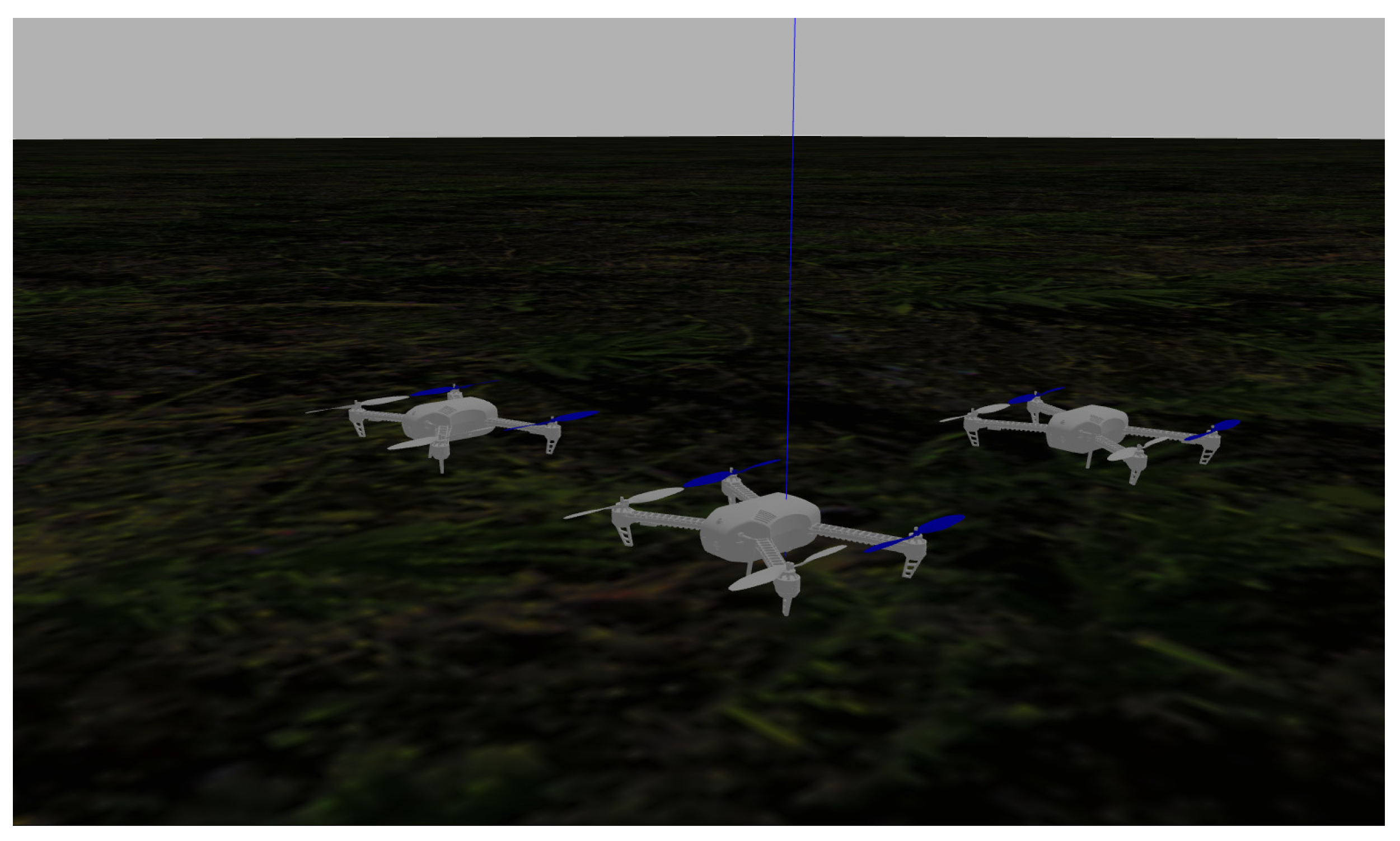
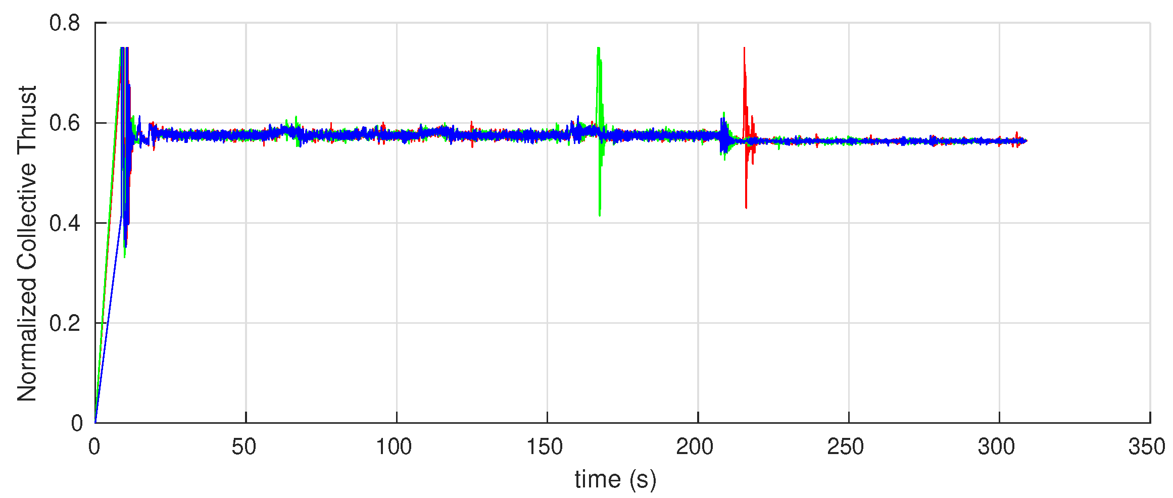
8.3. Software-in-the-Loop Simulations

The performance of the suggested sweeping coverage control for multi-quadrotor systems was evaluated using Software-in-the-Loop (SITL) simulations using Gazebo and the Robot Operating System (ROS) framework. This allows us to test the computational performance of the production code which can be used directly on the real vehicle’s onboard computer to implement our algorithms and control strategies in real-time. A simple scenario was considered where a group of three quadrotors were needed to survey a crops field S ˜ = { x , y , z I R : 0 x 32 , 0 y 40 , z = 0 } . Each vehicle is assumed to have an onboard camera providing a sensing footprint A i S dependent on its characteristics and the UAV’s altitude. For simplicity, an obstacle-free environment was used as shown in Figure 19.
We used the open-source PX4 flight stack as an implementation for the low-level controller and an extended Kalman filter for states estimation considering noisy measurements. Our tracking control logic was implemented using C++ providing thrust and attitude inputs at a rate of 100Hz. Furthermore, centroidal Voronoi configurations computations were implemented using Python utilizing some of the available tools from the "scipy.spatial" Python module to determine Voronoi cells as a convex polygon in accordance with Assumption 1. Furthermore, the algorithm in S1S4 was used to obtain the centroids. This turned out to be very computationally efficient since the computations rely on closed-form expressions.
In order to achieve the coverage task in hand, an initial rectangular sweeping plane was selected as: F ( 0 ) = { x , y , z I R : 0 x 8 , 0 y 2 , z = 2 } where it was required for the UAVs to fly at a fixed altitude of 2 m . The classical lawn-mower pattern was considered to generate the trajectory of F ( t ) to completely scan S ˜ while keeping the yaw angle at ψ r e f = 0 without loss of generality. The following parameters were used in the simulation: L 1 , i = d i a g { 2 , 2.5 , 3 } , L 2 , i = d i a g { 2.5 , 3 , 4 } , L i j = d i a g { 1 , 1 , 1 } , d c = 0.5 m , μ 1 = 2 and μ 2 = 1.5 (where d i a g { · } represents a diagonal matrix).
During the simulation, all measurements and data were captured as a bag file using available ROS recording tools. The results are plotted using MATLAB which are shown in Figure 20, Figure 21, Figure 22, Figure 23, Figure 24 and Figure 25. In Figure 20, coordinates of all vehicles are plotted with respect to time. The overall paths taken by the vehicles are shown in Figure 21 where the highlighted rectangular area represents the crops field to be surveyed (i.e., S ˜ ). Note that in this time, the vehicles were moving along some other region S whose projection on the ground floor is S ˜ . Thus, the trajectory of F ( t ) was designed to cover S ˜ given that the equipped sensors have a collective footprint which ensures the optimal coverage of S ˜ . It is clear from these results that the overall motion is collision-free, and the lawn-mower pattern decided for F ( t ) was followed by the whole group. Velocity norms are shown in Figure 23. Overall the vehicles are moving with a constant speed g 0 = 1 m / s except for some changes in velocity at times where the vehicles are turning ( t 60 s, 110 s,160 s) in order to avoid collisions with each others. Overall, velocities remain within the desired limits of v 3.5 m/s except at the start when vehicles were taking off which is based on a different control law. The high-level control commands, namely roll, pitch, yaw and thrust, are shown in Figure 24 and Figure 25 where the thrust is normalized in the range [ 0 , 1 ] . This simulation case shows that our control can be successfully implemented using multi-quadrotor systems.

9. Conclusions & Future Work

Distributed cooperative control methods were proposed in this paper for multi-UAV systems to address coverage problems in 3D spaces including barrier and sweeping problems. Additionally, a generalization of these approaches was given to address flocking problems. The development of control laws was based on general kinematic model which make them applicable to different UAV types and autonomous underwater vehicles as well. A region-based control mechanism was adopted to constrain the movement of the vehicles within some desired region providing a computationally efficient solution that is both robust and scalable. Mathematical analysis was performed to ensure the stability of the developed control laws. Several simulations have been performed confirming the performance of the developed methods for 3D static and dynamic coverage problems. Additional simulation cases were also presented to show how well the suggested approach can handle obstacle avoidance as well as being robust against vehicles’ failure. To evaluate the computational performance, software-in-the-loop simulations, using Gazebo and ROS, were also carried out considering a special case of using a multi-quadrotor system in precision agriculture. To that end, specific implementation details were also proposed based on quadrotor dynamics. Future work can consider practical implementation and developing proper ways where the vehicles can collaboratively decide the shape of the dynamic region based on the multi-UAV system characteristics and the targeted sensing region size.

Author Contributions

Conceptualization, T.E. and A.V.S.; methodology, T.E.; software, T.E.; validation, T.E.; formal analysis, T.E.; resources, A.V.S.; writing—original draft preparation, T.E.; writing—review and editing, A.V.S.; visualization, T.E.; supervision, A.V.S.; project administration, A.V.S.; funding acquisition, A.V.S. All authors have read and agreed to the published version of the manuscript.

Funding

This work was supported by the Australian Research Council. Furthermore, this work received funding from the Australian Government, via grant AUSMURIB000001 associated with ONR MURI grant N00014-19-1-2571.

Conflicts of Interest

The authors declare no conflict of interest.

References

  1. Cortes, J.; Martinez, S.; Karatas, T.; Bullo, F. Coverage control for mobile sensing networks. IEEE Trans. Robot. Autom. 2004, 20, 243–255. [Google Scholar] [CrossRef]
  2. Hussein, I.I.; Stipanovic, D.M. Effective coverage control for mobile sensor networks with guaranteed collision avoidance. IEEE Trans. Control. Syst. Technol. 2007, 15, 642–657. [Google Scholar] [CrossRef]
  3. Pimenta, L.C.A.; Kumar, V.; Mesquita, R.C.; Pereira, G.A.S. Sensing and coverage for a network of heterogeneous robots. In Proveedings of the 2008 47th IEEE Conference on Decision and Control, Cancun, Mexico, 9–11 December 2008; IEEE: Manhattan, NY, USA, 2008; pp. 3947–3952. [Google Scholar]
  4. Cheng, T.M.; Savkin, A.V. A distributed self-deployment algorithm for the coverage of mobile wireless sensor networks. IEEE Commun. Lett. 2009, 13, 877–879. [Google Scholar] [CrossRef]
  5. Schwager, M.; Rus, D.; Slotine, J.J. Decentralized, adaptive coverage control for networked robots. Int. J. Robot. Res. 2009, 28, 357–375. [Google Scholar] [CrossRef] [Green Version]
  6. Cheng, T.M.; Savkin, A.V. Decentralized control for mobile robotic sensor network self-deployment: Barrier and sweep coverage problems. Robotica 2011, 29, 283–294. [Google Scholar] [CrossRef]
  7. Stergiopoulos, Y.; Thanou, M.; Tzes, A. Distributed collaborative coverage-control schemes for non-convex domains. IEEE Trans. Autom. Control. 2015, 60, 2422–2427. [Google Scholar] [CrossRef]
  8. Savkin, A.V.; Cheng, T.M.; Xi, Z.; Javed, F.; Matveev, A.S.; Nguyen, H. Decentralized Coverage Control Problems for Mobile Robotic Sensor and Actuator Networks; John Wiley & Sons: Hoboken, NJ, USA, 2015. [Google Scholar]
  9. Chao, H.; Baumann, M.; Jensen, A.; Chen, Y.; Cao, Y.; Ren, W.; McKee, M. Band-reconfigurable multi-UAV-based cooperative remote sensing for real-time water management and distributed irrigation control. IFAC Proc. Vol. 2008, 41, 11744–11749. [Google Scholar] [CrossRef]
  10. Hu, J.; Yang, J. Application of distributed auction to multi-UAV task assignment in agriculture. Int. J. Precis. Agric. Aviat. 2018, 1. [Google Scholar] [CrossRef] [Green Version]
  11. Ju, C.; Son, H. Multiple UAV systems for agricultural applications: Control, implementation, and evaluation. Electronics 2018, 7, 162. [Google Scholar] [CrossRef] [Green Version]
  12. Maes, W.H.; Steppe, K. Perspectives for remote sensing with unmanned aerial vehicles in precision agriculture. Trends Plant Sci. 2019, 24, 152–164. [Google Scholar] [CrossRef] [PubMed]
  13. Hegde, A.; Ghose, D. Multi-UAV Distributed Control for Load Transportation in Precision Agriculture. In Proceedings of the AIAA Scitech 2020 Forum, Orlando, FL, USA, 6–10 January 2020; p. 2068. [Google Scholar]
  14. Bernard, M.; Kondak, K.; Maza, I.; Ollero, A. Autonomous transportation and deployment with aerial robots for search and rescue missions. J. Field Robot. 2011, 28, 914–931. [Google Scholar] [CrossRef] [Green Version]
  15. Michael, N.; Fink, J.; Kumar, V. Cooperative manipulation and transportation with aerial robots. Auton. Robot. 2011, 30, 73–86. [Google Scholar] [CrossRef] [Green Version]
  16. Fink, J.; Michael, N.; Kim, S.; Kumar, V. Planning and control for cooperative manipulation and transportation with aerial robots. Int. J. Robot. Res. 2011, 30, 324–334. [Google Scholar] [CrossRef]
  17. Sreenath, K.; Kumar, V. Dynamics, control and planning for cooperative manipulation of payloads suspended by cables from multiple quadrotor robots. In Proceedings of the Robotics: Science and Systems IX, Berlin, Germany, 24–28 June 2013. [Google Scholar]
  18. Ruggiero, F.; Lippiello, V.; Ollero, A. Aerial manipulation: A literature review. IEEE Robot. Autom. Lett. 2018, 3, 1957–1964. [Google Scholar] [CrossRef] [Green Version]
  19. Arnold, R.D.; Yamaguchi, H.; Tanaka, T. Search and rescue with autonomous flying robots through behavior-based cooperative intelligence. J. Int. Humanit. Action 2018, 3, 1–18. [Google Scholar] [CrossRef] [Green Version]
  20. Hayat, S.; Yanmaz, E.; Bettstetter, C.; Brown, T.X. Multi-objective drone path planning for search and rescue with quality-of-service requirements. Auton. Robot. 2020, 44, 1183–1198. [Google Scholar] [CrossRef]
  21. Ausonio, E.; Bagnerini, P.; Ghio, M. Drone Swarms in Fire Suppression Activities: A Conceptual Framework. Drones 2021, 5, 17. [Google Scholar] [CrossRef]
  22. Li, X.; Savkin, A.V. Networked Unmanned Aerial Vehicles for Surveillance and Monitoring: A Survey. Future Internet 2021, 13, 174. [Google Scholar] [CrossRef]
  23. Xu, C.; Zhang, K.; Jiang, Y.; Niu, S.; Yang, T.; Song, H. Communication Aware UAV Swarm Surveillance Based on Hierarchical Architecture. Drones 2021, 5, 33. [Google Scholar] [CrossRef]
  24. Cole, D.T.; Thompson, P.; Göktoğan, A.H.; Sukkarieh, S. System development and demonstration of a cooperative UAV team for mapping and tracking. Int. J. Robot. Res. 2010, 29, 1371–1399. [Google Scholar] [CrossRef]
  25. Hu, J.; Xu, J.; Xie, L. Cooperative search and exploration in robotic networks. Unmanned Syst. 2013, 1, 121–142. [Google Scholar] [CrossRef]
  26. Mahdoui, N.; Frémont, V.; Natalizio, E. Communicating Multi-UAV System for cooperative SLAM-based exploration. J. Intell. Robot. Syst. 2020, 98, 325–343. [Google Scholar] [CrossRef] [Green Version]
  27. Gage, D.W. Command control for many-robot systems. Unmanned Syst. 1992, 10, 28–34. [Google Scholar]
  28. Atınç, G.M.; Stipanović, D.M.; Voulgaris, P.G. A swarm-based approach to dynamic coverage control of multi-agent systems. Automatica 2020, 112, 108637. [Google Scholar] [CrossRef]
  29. Olfati-Saber, R. Flocking for multi-agent dynamic systems: Algorithms and theory. IEEE Trans. Autom. Control. 2006, 51, 401–420. [Google Scholar] [CrossRef] [Green Version]
  30. Reynolds, C.W. Flocks, herds and schools: A distributed behavioral model. In ACM SIGGRAPH Computer Graphics; ACM: New York, NY, USA, 1987; Volume 21, pp. 25–34. [Google Scholar]
  31. Cortes, J.; Martinez, S.; Bullo, F. Spatially-distributed coverage optimization and control with limited-range interactions. ESAIM Control. Optim. Calc. Vars. 2005, 11, 691–719. [Google Scholar] [CrossRef] [Green Version]
  32. Barr, S.J.; Wang, J.; Liu, B. An Efficient Method for Constructing Underwater Sensor Barriers. J. Commun. 2011, 6, 370–383. [Google Scholar] [CrossRef]
  33. Petersen, I.R.; Savkin, A.V. Robust Kalman Filtering for Signals and Systems with Large Uncertainties; Birkhauser: Boston, MA, USA, 1999. [Google Scholar]
  34. Tipsuwan, Y.; Chow, M.Y. Control methodologies in networked control systems. Control. Eng. Pract. 2003, 11, 1099–1111. [Google Scholar] [CrossRef]
  35. Hespanha, J.P.; Naghshtabrizi, P.; Xu, Y. A survey of recent results in networked control systems. Proc. IEEE 2007, 95, 138–162. [Google Scholar] [CrossRef] [Green Version]
  36. Wang, F.Y.; Liu, D. Networked control systems: Theory and Applications; Springer: London, UK, 2008. [Google Scholar]
  37. Matveev, A.S.; Savkin, A.V. Estimation and Control over Communication Networks; Birkhauser Boston: Cambridge, MA, USA, 2009. [Google Scholar]
  38. Bemporad, A.; Heemels, M.; Johansson, M. Networked Control Systems; Springer: New York, NY, USA, 2010; Volume 406. [Google Scholar]
  39. Ge, X.; Yang, F.; Han, Q.L. Distributed networked control systems: A brief overview. Inf. Sci. 2017, 380, 117–131. [Google Scholar] [CrossRef]
  40. Davoli, L.; Pagliari, E.; Ferrari, G. Hybrid LoRa-IEEE 802.11s Opportunistic Mesh Networking for Flexible UAV Swarming. Drones 2021, 5, 26. [Google Scholar] [CrossRef]
  41. Cheah, C.C.; Hou, S.P.; Slotine, J.J.E. Region-based shape control for a swarm of robots. Automatica 2009, 45, 2406–2411. [Google Scholar] [CrossRef]
  42. Huang, S.; Teo, R.S.H.; Leong, W.W.L.; Martinel, N.; Forest, G.L.; Micheloni, C. Coverage control of multiple unmanned aerial vehicles: A short review. Unmanned Syst. 2018, 6, 131–144. [Google Scholar] [CrossRef]
  43. Kwok, A.; Martinez, S. Energy-balancing cooperative strategies for sensor deployment. In Proceedings of the 2007 46th IEEE Conference on Decision and Control, New Orleans, LA, USA, 12–14 December 2007; IEEE: Manhattan, NY, USA, 2007; pp. 6136–6141. [Google Scholar]
  44. Dieber, B.; Micheloni, C.; Rinner, B. Resource-aware coverage and task assignment in visual sensor networks. IEEE Trans. Circuits Syst. Video Technol. 2011, 21, 1424–1437. [Google Scholar] [CrossRef]
  45. Wang, X.; Han, S.; Wu, Y.; Wang, X. Coverage and energy consumption control in mobile heterogeneous wireless sensor networks. IEEE Trans. Autom. Control. 2012, 58, 975–988. [Google Scholar] [CrossRef]
  46. Morsly, Y.; Aouf, N.; Djouadi, M.S.; Richardson, M. Particle swarm optimization inspired probability algorithm for optimal camera network placement. IEEE Sens. J. 2011, 12, 1402–1412. [Google Scholar] [CrossRef]
  47. Abo-Zahhad, M.; Ahmed, S.M.; Sabor, N.; Sasaki, S. Rearrangement of mobile wireless sensor nodes for coverage maximization based on immune node deployment algorithm. Comput. Electr. Eng. 2015, 43, 76–89. [Google Scholar] [CrossRef]
  48. Wang, H.; Guo, Y. A decentralized control for mobile sensor network effective coverage. In Proceedings of the 2008 7th World Congress on Intelligent Control and Automation, Chongqing, China, 25–27 June 2008; IEEE: Manhattan, NY, USA, 2008; pp. 473–478. [Google Scholar]
  49. Howard, A.; Matarić, M.J.; Sukhatme, G.S. Mobile sensor network deployment using potential fields: A distributed, scalable solution to the area coverage problem. In Distributed Autonomous Robotic Systems 5; Springer: Tokyo, Japan, 2002; pp. 299–308. [Google Scholar]
  50. Schwager, M.; Vitus, M.P.; Rus, D.; Tomlin, C.J. Robust adaptive coverage for robotic sensor networks. In Robotics Research; Springer: New York, NY, USA, 2017; pp. 437–454. [Google Scholar]
  51. Stergiopoulos, Y.; Tzes, A. Autonomous deployment of heterogeneous mobile agents with arbitrarily anisotropic sensing patterns. In Proceedings of the 2012 20th Mediterranean Conference on Control & Automation (MED), Barcelona, Spain, 3–6 July 2012; IEEE: Manhattan, NY, USA, 2012; pp. 1585–1590. [Google Scholar]
  52. Stergiopoulos, Y.; Tzes, A. Cooperative positioning/orientation control of mobile heterogeneous anisotropic sensor networks for area coverage. In Proceedings of the 2014 IEEE International Conference on Robotics and Automation (ICRA), Hong Kong, China, 31 May–7 June 2014; IEEE: Manhattan, NY, USA, 2014; pp. 1106–1111. [Google Scholar]
  53. Kantaros, Y.; Zavlanos, M.M. Distributed communication-aware coverage control by mobile sensor networks. Automatica 2016, 63, 209–220. [Google Scholar] [CrossRef]
  54. Papatheodorou, S.; Tzes, A.; Stergiopoulos, Y. Collaborative visual area coverage. Robot. Auton. Syst. 2017, 92, 126–138. [Google Scholar] [CrossRef] [Green Version]
  55. Thanou, M.; Tzes, A. Distributed visibility-based coverage using a swarm of UAVs in known 3D-terrains. In Proceedings of the 2014 6th International Symposium on Communications, Control and Signal Processing (ISCCSP), Athens, Greece, 21–23 May 2014; IEEE: Manhattan, NY, USA, 2014; pp. 425–428. [Google Scholar]
  56. Hexsel, B.; Chakraborty, N.; Sycara, K. Coverage control for mobile anisotropic sensor networks. In Proceedings of the 2011 IEEE International Conference on Robotics and Automation, Shanghai, China, 9–13 May 2011; IEEE: Manhattan, NY, USA, 2011; pp. 2878–2885. [Google Scholar]
  57. Mohapatra, S.K.; Sahoo, P.K.; Wu, S.L. Big data analytic architecture for intruder detection in heterogeneous wireless sensor networks. J. Netw. Comput. Appl. 2016, 66, 236–249. [Google Scholar] [CrossRef]
  58. Saeed, A.; Abdelkader, A.; Khan, M.; Neishaboori, A.; Harras, K.A.; Mohamed, A. Argus: Realistic target coverage by drones. In Proceedings of the 16th ACM/IEEE International Conference on Information Processing in Sensor Networks, Pittsburgh, PA, USA, 18–21 April 2017; IEEE: Manhattan, NY, USA, 2017; pp. 155–166. [Google Scholar]
  59. Bullo, F.; Cortés, J.; Martinez, S. Distributed Control of Robotic Networks: A Mathematical Approach to Motion Coordination Algorithms; Princeton University Press: Princeton, NJ, USA, 2009. [Google Scholar]
  60. Bhattacharya, S.; Ghrist, R.; Kumar, V. Multi-robot coverage and exploration on Riemannian manifolds with boundaries. Int. J. Robot. Res. 2014, 33, 113–137. [Google Scholar] [CrossRef]
  61. Panagou, D.; Stipanović, D.M.; Voulgaris, P.G. Vision-based dynamic coverage control for nonholonomic agents. In Proceedings of the 53rd IEEE Conference on Decision and Control, Los Angeles, CA, USA, 15–17 December 2014; IEEE: Manhattan, NY, USA, 2014; pp. 2198–2203. [Google Scholar]
  62. Panagou, D.; Stipanović, D.M.; Voulgaris, P.G. Distributed dynamic coverage and avoidance control under anisotropic sensing. IEEE Trans. Control. Netw. Syst. 2016, 4, 850–862. [Google Scholar] [CrossRef]
  63. Li, W.T.; Liu, Y.C. Dynamic coverage control for mobile robot network with limited and nonidentical sensory ranges. In Proceedings of the 2017 IEEE International Conference on Robotics and Automation (ICRA), Singapore, 29 May–3 June 2017; IEEE: Manhattan, NY, USA, 2017; pp. 775–780. [Google Scholar]
  64. Zuo, L.; Shi, Y.; Yan, W. Dynamic coverage control in a time-varying environment using Bayesian prediction. IEEE Trans. Cybern. 2017, 49, 354–362. [Google Scholar] [CrossRef] [PubMed]
  65. Song, C.; Liu, L.; Feng, G.; Wang, Y.; Gao, Q. Persistent awareness coverage control for mobile sensor networks. Automatica 2013, 49, 1867–1873. [Google Scholar] [CrossRef]
  66. Bhattacharya, S.; Michael, N.; Kumar, V. Distributed coverage and exploration in unknown non-convex environments. In Distributed Autonomous Robotic Systems; Springer: New York, NY, USA, 2013; pp. 61–75. [Google Scholar]
  67. Wang, Y.; Liu, Y.; Guo, Z. Three-dimensional ocean sensor networks: A survey. J. Ocean. Univ. China 2012, 11, 436–450. [Google Scholar] [CrossRef]
  68. Bentz, W.; Panagou, D. 3D dynamic coverage and avoidance control in power-constrained UAV surveillance networks. In Proceedings of the 2017 International Conference on Unmanned Aircraft Systems (ICUAS), Miami, FL, USA, 13–16 June 2017; IEEE: Manhattan, NY, USA, 2017; pp. 1–10. [Google Scholar]
  69. Bentz, W.; Hoang, T.; Bayasgalan, E.; Panagou, D. Complete 3-D dynamic coverage in energy-constrained multi-UAV sensor networks. Auton. Robot. 2018, 42, 825–851. [Google Scholar] [CrossRef]
  70. Pompili, D.; Melodia, T.; Akyildiz, I.F. Deployment analysis in underwater acoustic wireless sensor networks. In Proceedings of the 1st ACM international workshop on Underwater Networks, Los Angeles, CA, USA, 25 September 2006; ACM: New York, NY, USA, 2006; pp. 48–55. [Google Scholar]
  71. Stirling, T.; Wischmann, S.; Floreano, D. Energy-efficient indoor search by swarms of simulated flying robots without global information. Swarm Intell. 2010, 4, 117–143. [Google Scholar] [CrossRef]
  72. Boufares, N.; Khoufi, I.; Minet, P.; Saidane, L.; Saied, Y.B. Three dimensional mobile wireless sensor networks redeployment based on virtual forces. In Proceedings of the 2015 International Wireless Communications and Mobile Computing Conference (IWCMC), Dubrovnik, Croatia, 24–28 August 2015; IEEE: Manhattan, NY, USA, 2015; pp. 563–568. [Google Scholar]
  73. Nazarzehi, V.; Savkin, A.V. Distributed self-deployment of mobile wireless 3D robotic sensor networks for complete sensing coverage and forming specific shapes. Robotica 2018, 36, 1–18. [Google Scholar] [CrossRef]
  74. Tanner, H.G.; Jadbabaie, A.; Pappas, G.J. Flocking in fixed and switching networks. IEEE Trans. Autom. Control. 2007, 52, 863–868. [Google Scholar] [CrossRef]
  75. Dimarogonas, D.V.; Kyriakopoulos, K.J. A connection between formation infeasibility and velocity alignment in kinematic multi-agent systems. Automatica 2008, 44, 2648–2654. [Google Scholar] [CrossRef]
  76. Savkin, A.V.; Teimoori, H. Decentralized navigation of groups of wheeled mobile robots with limited communication. IEEE Trans. Robot. 2010, 26, 1099–1104. [Google Scholar] [CrossRef]
  77. Reyes, L.A.V.; Tanner, H.G. Flocking, formation control, and path following for a group of mobile robots. IEEE Trans. Control. Syst. Technol. 2015, 23, 1268–1282. [Google Scholar] [CrossRef]
  78. Khaledyan, M.; Liu, T.; Fernandez-Kim, V.; de Queiroz, M. Flocking and target interception control for formations of nonholonomic kinematic agents. IEEE Trans. Control. Syst. Technol. 2019, 28, 1603–1610. [Google Scholar] [CrossRef] [Green Version]
  79. Do, K.D. Flocking for multiple elliptical agents with limited communication ranges. IEEE Trans. Robot. 2011, 27, 931–942. [Google Scholar] [CrossRef]
  80. Antonelli, G.; Arrichiello, F.; Chiaverini, S. Flocking for multi-robot systems via the null-space-based behavioral control. Swarm Intell. 2010, 4, 37. [Google Scholar] [CrossRef]
  81. Virágh, C.; Vásárhelyi, G.; Tarcai, N.; Szörényi, T.; Somorjai, G.; Nepusz, T.; Vicsek, T. Flocking algorithm for autonomous flying robots. Bioinspiration Biomim. 2014, 9, 025012. [Google Scholar] [CrossRef] [Green Version]
  82. Ghapani, S.; Mei, J.; Ren, W.; Song, Y. Fully distributed flocking with a moving leader for Lagrange networks with parametric uncertainties. Automatica 2016, 67, 67–76. [Google Scholar] [CrossRef] [Green Version]
  83. Jafari, M.; Xu, H. A biologically-inspired distributed fault tolerant flocking control for multi-agent system in presence of uncertain dynamics and unknown disturbance. Eng. Appl. Artif. Intell. 2019, 79, 1–12. [Google Scholar] [CrossRef]
  84. Hamel, T.; Mahony, R.; Lozano, R.; Ostrowski, J. Dynamic modelling and configuration stabilization for an X4-flyer. IFAC Proc. Vol. 2002, 35, 217–222. [Google Scholar] [CrossRef]
  85. Mellinger, D.; Kumar, V. Minimum snap trajectory generation and control for quadrotors. In Proceedings of the 2011 IEEE International Conference on Robotics and Automation, Shanghai, China, 9–13 May 2011; IEEE: Manhattan, NY, USA, 2011; pp. 2520–2525. [Google Scholar]
  86. Faessler, M.; Franchi, A.; Scaramuzza, D. Differential flatness of quadrotor dynamics subject to rotor drag for accurate tracking of high-speed trajectories. IEEE Robot. Autom. Lett. 2017, 3, 620–626. [Google Scholar] [CrossRef] [Green Version]
Figure 1. Example Voronoi partition of a 2D plane divided into number of regions with their associated points.
Drones 05 00124 g001
Figure 10. UAV locations at different time instants showing the robustness of the proposed approach against UAVs failures when they get removed from the group (Simulation Case 5).
Drones 05 00124 g010aDrones 05 00124 g010b
Figure 11. Complete trajectories of the Multi-UAV system showing both active and inactive UAVs (Simulation Case 5).
Drones 05 00124 g011
Figure 12. UAV locations at different time instants showing the obstacle avoidance capability of the proposed approach by dynamically manipulating the sweeping plane F ( t ) (Simulation Case 6).
Drones 05 00124 g012aDrones 05 00124 g012b
Figure 13. Complete trajectories of the Multi-UAV system showing the obstacle avoidance capability of the proposed approach [Planar Views] (Simulation Case 6).
Drones 05 00124 g013
Figure 14. Complete trajectories of the Multi-UAV system showing the obstacle avoidance capability of the proposed approach [3D View] (Simulation Case 6).
Drones 05 00124 g014
Figure 15. Multi-Region simulation case 1 ( n = 100 and m = 10 ).
Drones 05 00124 g015
Figure 16. Multi-Region simulation case 2 ( n = 100 and m = 10 ).
Drones 05 00124 g016
Figure 17. Multi-Region simulation case 3 ( n = 108 and m = 6 ).
Drones 05 00124 g017
Figure 18. Multi-Region simulation case 1 ( n = 40 and m = 5 ).
Drones 05 00124 g018
Figure 19. UAVs and environment used in simulations.
Drones 05 00124 g019
Figure 20. UAVs coordinates with respect to time.
Drones 05 00124 g020
Figure 21. UAVs actual trajectories (3D prospective).
Drones 05 00124 g021
Figure 22. UAVs actual trajectories (2D prospective).
Drones 05 00124 g022
Figure 23. UAVs linear velocities with respect to time.
Drones 05 00124 g023
Figure 24. UAVs attitude (roll, pitch and yaw) with respect to time.
Drones 05 00124 g024
Figure 25. UAVs normalized collective thrust input with respect to time.
Drones 05 00124 g025
Publisher’s Note: MDPI stays neutral with regard to jurisdictional claims in published maps and institutional affiliations.

