Article

Monitoring Selective Logging in a Pine-Dominated Forest in Central Germany with Repeated Drone Flights Utilizing A Low Cost RTK Quadcopter

1
German Aerospace Center, Institute of Data Science, Maelzerstraße 3, 07743 Jena, Germany
2
Friedrich-Schiller-University, Department for Earth Observation, Loebdergraben 32, 07743 Jena, Germany
3
Friedrich-Schiller-University, Department for Physical Geography, Loebdergraben 32, 07743 Jena, Germany
*
Author to whom correspondence should be addressed.
Drones 2020, 4(2), 11; https://doi.org/10.3390/drones4020011
Submission received: 5 February 2020 / Revised: 30 March 2020 / Accepted: 5 April 2020 / Published: 9 April 2020

Abstract

:
There is no doubt that unmanned aerial systems (UAS) will play an increasing role in Earth observation in the near future. The field of application is very broad and includes aspects of environmental monitoring, security, humanitarian aid, or engineering. In particular, drones with camera systems are already widely used. The capability to compute ultra-high-resolution orthomosaics and three-dimensional (3D) point clouds from UAS imagery generates a wide interest in such systems, not only in the science community, but also in industry and agencies. In particular, forestry sciences benefit from ultra-high-structural and spectral information as regular tree level-based monitoring becomes feasible. There is a great need for this kind of information as, for example, due to the spring and summer droughts in Europe in the years 2018/2019, large quantities of individual trees were damaged or even died. This study focuses on selective logging at the level of individual trees using repeated drone flights. Using the new generation of UAS, which allows for sub-decimeter-level positioning accuracies, a change detection approach based on bi-temporal UAS acquisitions was implemented. In comparison to conventional UAS, the effort of implementing repeated drone flights in the field was low, because no ground control points needed to be surveyed. As shown in this study, the geometrical offset between the two collected datasets was below 10 cm across the site, which enabled a direct comparison of both datasets without the need for post-processing (e.g., image matching). For the detection of logged trees, we utilized the spectral and height differences between both acquisitions. For their delineation, an object-based approach was employed, which was proven to be highly accurate (precision = 97.5%; recall = 91.6%). Due to the ease of use of such new generation, off-the-shelf consumer drones, their decreasing purchase costs, the quality of available workflows for data processing, and the convincing results presented here, UAS-based data can and should complement conventional forest inventory practices.

Graphical Abstract

1. Introduction

“Drones-the third generation source of remote sensing data” was chosen as the title for the leading article by [1] for the special issue on Unmanned Aerial Systems (UAS) in the International Journal of Remote Sensing. The title is based on the idea that, after the implementation and operationalization of airborne and spaceborne platforms, UAS emerged as a new source of valuable Earth observation data. These data are capable of closing the gap between in-situ and far range remote sensing data, and thus allow for new developments of data scaling approaches [2]. Most UAS are equipped with optical camera systems providing imagery with ultra-high (i.e., centimeter scale) spatial resolution. Well-established photogrammetric processing chains, often summarized as structure from motion (SfM), exist to compute three-dimensional (3D) point clouds and orthomosaics based on overlapping UAS imagery [3]. Their high flexibility and accessibility (data acquisition at almost any time), scalability (choice of spatial resolution and areal coverage), and ease of use has led to an increased use of UAS for many applications and topics such as agriculture [4,5], forestry [6], geology [7], archeology [8], structural health monitoring [9], topographic surveying [10], and general mapping [1]. In the past years, this tendency has been facilitated by the advent of low-cost, off-the-shelf consumer drones with simple handling. Such drones have also pushed the wide use of UAS data for citizen science or humanitarian crowdsourcing organizations such as the UAViators (www.uaviators.org). Recently, low-cost UAS featuring real-time kinematic (RTK)-based positioning systems have emerged. Such RTK UAS allow for imagery with positional accuracy better than 5 cm and, thus, precise direct georeferencing. Accordingly, for several applications, the surveying of ground control points (GCPs) might become obsolete, saving costs and time.
This study is based on these recent technological advances. The main aim of this study was to test the capability of a low-cost RTK quadcopter for the mapping of selective logging and to monitor forest management activities based on bi-temporal drone flights without using GCPs. For achieving this goal, a simple and robust object-based image analysis (OBIA)-based approach was developed. This approach uses spectral and height information. To our knowledge, this is the first time selective logging has been mapped based on repeated drone flights.

1.1. Relevant Methodological and Technical Background

1.1.1. Structure from Motion Processing Sequence

In UAS-based photogrammetry, the SfM approach [3], based on stereoscopic principles, is commonly used. SfM enables the simultaneous estimation of constant imaging properties, the motion of a single camera, as well as 3D object information. It involves three main steps: (1) the detection of noticeable image features/points in overlapping images, (2) the calculation of an initial imaging geometry and the corresponding sparse 3D point cloud, and (3) the optimization of the model as a whole. Firstly, salient image points are detected [11], localized, and matched in all images. Although Scale Invariant Feature Transform (SIFT) [12] is commonly used for point localization and matching, alternative approaches, outperforming SIFT in some instances, are emerging [13]. In the second step, the relative orientation of image pairs is estimated based on the corresponding salient image points detected previously, e.g., by using the calibrated minimal five-point algorithm [14]. For the identification of wrong point correspondences, Random Sample Consensus (RANSAC) approaches are used. For these methods, a minimal set of point correspondences are selected, e.g., randomly [15]. This set is used to compute a hypothesis for the desired solution. The remaining correspondences are checked regarding their support for the hypothesis, and this process is iterated several times to find the hypothesis with the highest support. The final solution is then estimated using this hypothesis and all inliers. By means of this method, image pairs are sequentially connected to a global network of all stereo image pairs. This network typically exhibits local tensions that can be reduced by a global bundle adjustment (BA) [16]. Finally, the refined sparse 3D point cloud can be densified by applying dense stereo matching methods [17].
According to the SfM processing chain, the same points need to be identified in at least two images to form a correspondence (and potentially a tie point). In areas with a high chance of occlusion (such as forests), this issue can have an impact on the distribution of the tie points and the points of the sparse point cloud. Points representing the forest floor are scarce or even non-existent, although single images feature parts of the forest floor. Accordingly, as an approach utilizing passive optical data, SfM encompasses some limitations that can be partly avoided when working with laser-based systems, as discussed in Section 1.4.

1.1.2. The 3D Positional Accuracy of SfM Models

The 3D positional accuracy of point clouds and products derived from UAS imagery heavily depends on the UAS survey parameters (flight pattern, camera viewing angle, distribution of GCPs) and the SfM processing parameters [10,18,19]. For a weak network of tie points, as commonly achieved with parallel flight tracks and nadir images, systematic errors such as doming of the model frequently occur [18]. This effect can either be mitigated by using sufficient and well-distributed GCPs, or by using more complex flight patterns, including oblique images [10,18,19]. The surveyed GCPs also provide the basis for the absolute orientation and scale of the model within the external (e.g., geographic) coordinate system. In the absence of GCPs, absolute orientation can be achieved by direct georeferencing, for which the camera positions of the acquired images need to be measured during the flight campaign. As most UAS are equipped with global navigation satellite system (GNSS) receivers, camera positions are commonly available. Nevertheless, the absolute positional accuracy of the final SfM model is limited by the accuracy of the GNSS. Accordingly, for change detection approaches with UAS imagery, GNSS-based direct georeferencing is impeded, if not impossible, due to the positional offset between the repeated acquisitions. This, in turn, means that GCPs are mandatory when UAS equipped with a standard GNSS are used. However, GCP visibility in forested regions is hindered by the forest canopy, and is usually limited to forest stand gaps. Also, GNSS-based GCP surveying underneath a dense forest canopy is commonly not feasible, due to GNSS signal attenuation. Thanks to recent technological advances, these limitations have been overcome by the availability of a new generation of UAS. These systems feature hardware for RTK-based positioning and enable very high positional accuracies (better than 5 cm). The final SfM models are highly accurate as well, and thus allow for reliable direct georeferencing results. Additionally, systematic errors, as mentioned above, can be avoided [19].

1.2. UAS SfM Data-Based Tree Detection

The capability of UAS imaging systems to generate ultra-high-resolution imagery and 3D data holds great potential for the development of forestry applications. This is expressed in a large number of recent publications, such as [6,20,21,22,23,24,25,26,27,28,29,30,31,32]. According to [6], these publications focus on the estimation of dendrometric parameters, including height measurements, tree species classification, quantification of spatial gaps in forests, forest fire-related issues, forest health monitoring, and forest disease mapping. One of the main advantages of ultra-high-resolution data is the capability of tree-level-based analyses and applications. For the detection of individual trees, Zhen et al. [33] distinguished four groups of methods, namely, (1) raster-based methods (treetop detection, crown delineation, object-based image analysis (OBIA)); (2) point cloud-based methods (clustering, voxel-based segmentation); (3) methods combining raster, point clouds, and a priori information; and (4) tree shape reconstruction methods (e.g., convex hull, Hough transformation). Tree top detection involves algorithms such as local maximum, image binarization, and template matching, while crown delineation comprises valley-following, watershed segmentation, and region-growing. In general, the source of the point cloud or raster data is not relevant for the choice of one of these methods. Thus, these methods are also applicable to laser-based data (see below).
Several SfM data-based studies aimed at individual tree detection have used a local maxima approach [25,26,30,32]. In a study by Mohan et al. [25], UAS SfM-based point clouds were used for individual tree detection in a mixed conifer forest (Wyoming, USA). Thiel et al. [32] also used UAS imagery and SfM-based point clouds for a test site in Germany, which is part of the forest stand investigated in this study. Nevalainen et al. [30] aimed at individual tree detection and classification using UAS SfM-based point clouds and hyperspectral imaging in southern Finland, in which they used forest stands dominated by pine, spruce, birch, and larch. The study by Li et al. [26] applied a local maximum algorithm to delineate individual trees in the Huailai area, China. The task was to detect tree individuals (Aspen) forming windbreaks surrounding agricultural areas. However, in general, using multitemporal point clouds for change detection of forests is rarely reported in the literature.

1.3. Laser Scanner-Based Tree Detection

Although this work is based on UAS SfM data, our results are also discussed in the context of outcomes based on airborne light detection and ranging (LiDAR) [34] and terrestrial laser scanner (TLS) data [35], as there is hardly any related work published based on UAS SfM data. Both TLS and LiDAR are active laser scanning systems used for the generation of point clouds [36]. As active systems, laser scanners are independent of illumination conditions. Still, occlusion occurs, as the laser light cannot penetrate through optically dense materials. Nevertheless, occlusion is less prominent when compared to SfM, as each 3D point is measured directly. LiDAR systems can be mounted on aircraft, UAS, or ground-based platforms (vehicles, tripods, handheld systems, etc.). Professional LiDARs are capable of generating very precise and dense point clouds [35]. Also, the system specifications of the laser scanners allow for a proper assessment of the data quality in terms of positional accuracy. Due to their high cost, such devices are rarely available, and flexible use can hardly be guaranteed. Also, particularly in forests, the acquisition of TLS data is extremely time consuming and the surveyed areas are small. The area of acquisition can be extended when laser scanners are mounted on vehicles [37]. Still, limitations exist in terms of the requirement of traversable forest tracks, although these limitations can be overcome when laser scanners are mounted on UAS [38,39]. Due to the wide scanning angle, the high point cloud density, and the possibility to fly tracks with great overlap between the scans, shadowing hardly occurs. In contrast to conventional airborne LiDAR and UAS-borne SfM point clouds, stems can be sensed precisely [40]. Although the full potential of UAS-borne LiDAR is not yet fully exploited, similar tree detection rates achievable with multiple TLS scans can be expected, with the advantage of capturing larger areas in a shorter time, while having no GNSS constraints [38,40]. Nevertheless, it is questionable whether UAS-borne LiDAR systems will be widely used in the near future for the detection of selective logging. Professional systems are still very expensive, the data processing is complex, and the operation and handling of the hardware in the field is challenging.

1.3.1. LiDAR-Based Tree Detection

Multitemporal LiDAR point cloud-based change detection at the individual tree level is hardly reported in the literature. Limitations exist due to non-regular acquisitions and the enduring evolution of LiDAR sensors, resulting in increasing point densities and thus complications when comparing two dissimilar datasets. Nevertheless, in the work of Marinelli et al. [41,42] a new approach for selective logging using multitemporal LiDAR data in forest areas was proposed and tested in the Trento province of the southern Alps. The two test sites were covered by needle-leaved forest, and the point density of the LiDAR data ranged from 10 to 50 pls/m2, with four returns for each pulse. One benefit of the used LiDAR dataset in [41,42] is the high point density, and thus the high probability to receive ground returns even for small gaps in the canopy.
Other studies focused on individual tree detection and thus used monotemporal datasets. Nevertheless, the results of those studies enable the assessment of the accuracy of the change detection case. Under the assumption that the same method to detect selective logging is applied twice (using data acquired at different times), the accuracy of the change product can be estimated by squaring the accuracy of the monotemporal product. In the study by Lu et al. [43], a LiDAR-based approach was proposed, aiming at the segmentation of individual trees. This publication also presents a short collection of previously published results by various authors applying different individual tree segmentation methods. However, it is not feasible to draw conclusions regarding the preferable tree segmentation method, since the experimental setup varies significantly between the studies considered (e.g., point density, forest types). The bottom-up approach presented by Lu et al. [43] can detect 84% of the trees for a study site in Pennsylvania, USA dominated by a deciduous species (leaf-off). The point density was approximately 10 pls/m2, with up to four returns per pulse. Mongus and Zalik [44] presented an approach for 3D single tree crown delineation with LiDAR data by utilizing the complementaries of treetop and trunk detections. Six dissimilar test sites were selected, which were located in the Slovenian Alps, and the LiDAR point density ranged from 26 to 97 pts/m2 for the different sites. Hu et al. [45] developed a tree clustering algorithm based on the mean shift theory. The algorithm was applied to LiDAR data, with an average point density of 15 pts/m2 acquired over a multi-layered, evergreen broad-leaved forest in South China. Further publications on airborne LiDAR-based tree detection focus on the benchmarking of diverse methods [34], comparing vector- and raster-based segmentation approaches [36], or else try to identify trends in automatic individual crown detection [33]. With regard to the accuracy achieved, the results presented in these publications are in the same range as the previously cited studies.

1.3.2. Terrestrial Laser Scanner (TLS)-Based Tree Detection

Except the study by Mongus and Zalik [44], the previously discussed publications relied on canopy information for individual tree detection, and thus were prone to errors, as discussed in Section 4.1. below. One strategy to overcome this drawback is to sense the tree stems using TLS. TLS can generate 3D point cloud data with a much higher density than that achievable with airborne LiDAR. Thus, the sampling rate is commonly no limiting factor. The fastest TLS data acquisition and preprocessing strategy uses single scans, as shown by Liang et al. [46]. However, single scans only sense the stems from one side, therefore complicating data evaluation. According to Liang et al. [46], one main source of error is related to the trees standing close together. The study by Xia et al. [47] was also based on single scan data. Their site was located in the Sichuan Giant Panda Sanctuaries, China, and covered by mature and dense bamboo forest. The presented method was based on point clustering and merging a stem model afterwards. Shadowing, which is a typical phenomenon in single scan data, was discussed as the main source of error. In Oveland et al. [48], low-cost TLS equipment generating comparably low-density point clouds was tested in the Gran municipality in southeastern Norway, the forest of which is dominated by Norway spruce and Scots pine. The authors concluded that challenging GNSS conditions under forest canopies need to be treated accordingly. Multiple TLS scans were used by Maas et al. [49] to detect trees and to delineate the parameters relevant to the forest inventory. Five different test plots located in Austria and Ireland were chosen for this analysis, and the detection rate was much improved against the previous studies, which emphasizes the advantages of multiple scan data against single scans. A similar performance was achieved by Bienert et al. [37] for multiple scan datasets in the Lauerholz Forest, Northern Germany.

1.4. Organization of The Paper

The remainder of the paper is structured as follows: Section 2 presents the materials and methods, including a description of site, fieldwork, UAS data processing, reference data collection, method development, and framework of separability and accuracy analysis. Section 3 lays out the results, including separability and accuracy analysis. Section 4 presents the discussion, followed by the conclusion in Section 5.

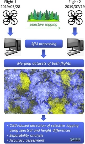
2. Materials and Methods

This chapter provides all of the necessary details on the site characteristics, the acquisition and processing of the UAS and other field data, the collection of reference data, the approach to detect felled trees, the approach to investigate the separability of the felled and remaining trees, and the accuracy analysis for the detection of felled trees.
Figure 1 shows the general workflow of this study. UAS imagery was recorded before and after the logging of individual trees. By means of SfM, orthomosaics and point clouds were computed using the acquired imagery. Based on the point clouds canopy height models (CHMs) were generated. The OBIA-based detection of felled trees is based on the spectral differences and CHM differences between both acquisition dates. The accuracy assessment refers to the detection rate of felled trees, and also includes false-positive and false-negative events. For gaining deeper insights into the data characteristics, the separability between the felled and the remaining trees was analyzed using various approaches.

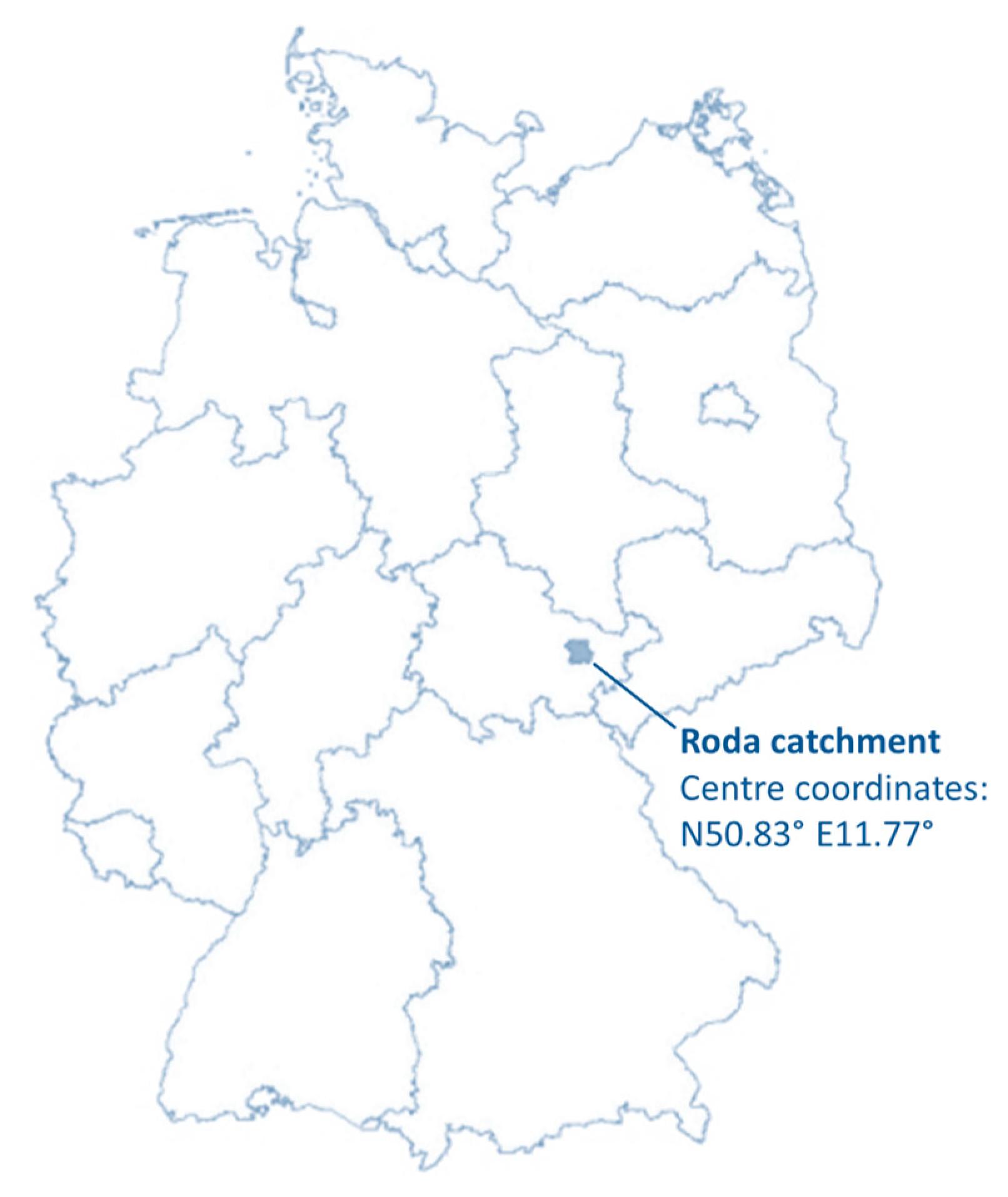
2.1. The Site “Roda Forest”

The Roda Forest is located in the federal state of Thuringia in Central Germany. It is part of the Roda River catchment (Figure 2) and is, for the most part, planted and intensively managed. The area of investigation (AOI) is located in the southern part of the Roda Forest. It has an extent of approximately 500 m × 250 m (Figure 3). The UAS mission covers a larger area of 0.465 km2, and the AOI is located in the center of the of the UAS mission area. The dominant tree species of the test site is Scots pine (Pinus sylvestris), followed by Norway spruce (Picea abies), and other rarely occurring species such as European larch (Larix decidua), birch (Betula pendula), and European beech (Fagus sylvatica). The stand is homogeneous in terms of tree age, while the tree density and height show some variability, in part due to past disturbances and slightly differing growing conditions (Figure 2 and Figure 3). The available forest inventory data provide stand-wise averages of relevant information (such as tree height, species compositions, relative stocking, etc.). Due to the incomplete canopy coverage (glades, gaps between trees), undergrowth is well-developed in some places. It comprises, amongst others, small trees (up to 8 m), bushes, bracken, and blackberry. The AOI features gentle terrain with elevations between 385 and 390 m (over WGS84 ellipsoid). The underlying bedrock (Early Trias–bunter) causes slightly acidic soils.
During the past two years, the forest of the AOI was affected by several stressors, such as storm events, bark beetle attacks, as well as long drought periods during the spring and summer of 2018 and the spring of 2019. Accordingly, several damages were obvious within the test site. Forest management activities were conducted in June 2019 to remove stressed and affected trees. Another intention of these activities was the slight thinning of the forest. Accordingly, trees were often cleared in areas with a high tree density.

2.2. Field Work: Acquisition of UAS Data and Check Points

The first UAS campaign took place on 28 May 2019 and the second on 19 July 2019. The logging activities were executed in between this time span. The UAS imagery was recorded using the RTK version of Da-Jiang Innovations Science and Technology Co., Ltd’s (DJI) Phantom 4 Pro. This system allows for very accurate real-time positioning in the order of centimeters (see Table 1), if correction data from a reference station can be received. For this study, the correction data stemmed from the German satellite positioning service SAPOS. The correction data were received via NTRIP (Networked Transport of RTCM (Radio Technical Commission for Maritime Services) via Internet Protocol). Accordingly, a mobile internet connection was required. The distance to the nearest SAPOS base station (reference station “JENA/Schoengleina”) was 14 km. As the RTK signal was constantly available during the flights, the positional accuracy can be expected to meet the specifications. The Phantom 4 Pro RTK is equipped with a camera featuring a 1″ CMOS (complementary metal oxide semiconductor) sensor and a mechanical shutter. The field of view of this system is 84°. The 3D RTK coordinate of the image center is stored in EXIF format, along with several other parameters. See Table 1 for further UAS specifications.
Both UAS campaigns were conducted under similar meteorological conditions (Table 2). Due to the very low wind speed, hardly any movements of the trees were observed during the flights. The full cloud coverage resulted in diffuse illumination conditions. Accordingly, unwanted effects, such as hard shadows and strong illumination differences between the canopy and the forest floor, were avoided. A simple airborne campaign-like flight pattern with parallel flight lines only was chosen. To increase the probability of detecting small glades and to obtain data from the forest floor, respectively, the images were acquired in nadir view and with a large image overlap (Table 2). According to the programmed flight speed, the shutter speed (fixed to 1/320 s), and the geometric ground resolution, motion blur was avoided. With respect to the aperture, the exposure value was set to −1 for the second flight campaign, as the illumination level was slightly reduced compared to the first campaign (denser cloud layer). By this means, similar aperture values were obtained for both campaigns. Take-off and landing were operated at the southern forest edge of the site. The visual observation of the UAS was possible from this position throughout the mission.
Although, for the SfM processing of the image data, only the camera positions and no GCPs were considered (direct georeferencing), five check points were placed to cover the area of interest (first campaign only). These equally distributed check points were used to evaluate the positional accuracy of the generated orthomosaic and digital elevation model (DEM). To precisely identify and locate the check points in the UAS imagery, 50 cm × 50 cm Teflon panels were utilized, featuring a black cross to mark the panel center. The positions of the Teflon panels were measured using survey grade equipment (ppm10xx-04 full RTK GNSS sensor in combination with Novatel Vexxis GNSS L1/L2-Antenna [51]). Each check point was surveyed 50 times. The root mean square error (RMSE; computed separately for x, y, z) was below 2 cm at all check points. For this study, the averaged positions of the 50 measurements were used.

2.3. UAS Data Processing

2.3.1. SfM-Based Generation of Orthomosaics and Point Clouds

The UAS data processing involved the computation of one dense 3D point cloud and one orthomosaic per UAS campaign. For the processing, the 3D reconstruction software Metashape 1.5.1 (Agisoft LLC) was used, applying the standard workflow. The UAS images were not altered before the SfM processing. Direct georeferencing was applied, and the camera positional accuracy parameter was set to 0.02 m (Table 3). For the processing of the UAS imagery of the second campaign, the camera model parameter set of the first campaign was applied. The rationale is that, due to the same campaign setup, the similar temperatures, and the similar aperture values, the physical camera structure should not have changed significantly, even though low-cost camera equipment was used. The validity of this assumption was confirmed after processing (see text below and Figure 4 and Figure 5). During the processing, all images could be aligned. The number of tie points was approximately 450,000 for both datasets. Both dense point clouds comprised about 66 million points, which corresponds to an average point density of 144 points/m2. According to the flight altitude and the camera hardware, the nominal geometric ground resolution was approximately 3 cm. Nevertheless, orthomosaics with 5 cm pixel spacing were produced, which can be considered as being sufficient for this study [32], as the objects to be detected are at least one magnitude larger. Figure 3 shows the orthomosaic of the first campaign.
At all check points, the deviation between the check point coordinate and the model coordinate was found to be below 5 cm (separately measured for x, y, z). The RMSE between the check points and the SfM model was below 2 cm. Further evidence for the high geometric quality of the SfM model was provided by the minor camera position error and the minor effective reprojection errors (Table 4).
The geometric alignment between the two models was checked for 18 objects distributed across the site. To this end, non-moving objects and stable targets were selected, such as deadwood on the forest floor, hunting stands, distinctive stones on the forest roads, or stacks of wood. The deviation between both models was below 10 cm for all objects (separately measured for x, y, z). The RMSE of the deviation at the 18 objects was below 2 cm. These numbers underline the advancement of RTK UAS against previous versions, with positional accuracy of several meters. To visualize the geometric agreement, bi-temporal composites are provided in Figure 5 and Figure 6. Figure 6 shows some trees that were felled between both UAS campaigns to demonstrate the potential of the radiometric information for change detection.

2.3.2. Computation of The Spectral Difference Images

Further UAS data processing comprised the computation of the difference between the orthomosaics of the first and the second UAS campaign (see Figure 1). This temporal difference was used as one of the predictors for the detection of felled trees. The difference image was filtered using simple averaging and a 15 × 15 filter matrix to remove the unwanted effects caused by slight misalignment, the movement of trees and tree elements, or small-scale changes. For an example of the filtered difference image, see Figure 7.

2.3.3. Computation of Canopy Height Models (CHM) and CHM Differences

A first look at the generated dense point clouds revealed one characteristic that potentially complicates the detection of logged trees using height information only. Although the UAS imagery was acquired in nadir and with a large overlap between the images, in several places, small gaps between trees were not detected correctly (see Figure 8). Nevertheless, the point cloud data were used to generate pit-free [53] CHMs using the command LAS2DEM of the point cloud processing software LAStools v181108 (see Figure 1). The chosen parameters are summarized in Table 5. This step utilizes the terrain-normalized UAS-based point clouds. For their normalization, LiDAR data provided by the Thuringian State Office for Property Management and Geographic Information, TLBG, acquired in February 2014 were available. The LiDAR returns were classified into ground and non-ground points with an average point density of 4 pts/m2. The data, including metadata, are freely available via the Thuringian Geoportal (www.geoportal-th.de).
In the next step, the elevation difference between both CHMs was computed (Figure 1). Figure 9 shows the difference image for the entire study area. In general, logged trees can be identified due to notable height differences of several meters. Due to the phenomenon described above, and the visualization in Figure 8, for many logged trees, the height difference was obviously underestimated. Still, the CHM difference can be used to indicate the position of logged trees. However, the operational detection becomes more challenging as height differences of this magnitude are also caused by other impacts, such as movement of vegetation due to wind, growth, or changes in the undergrowth caused by the harvesters (see, e.g., the northern edge of the study site in Figure 9).

2.4. Collection of Reference Data for Accuracy Assessment and Samples for Separability Analysis

For a subset of the test site containing approximately 200 trees, the trunk base coordinates of all of trees were available. The trunk base coordinates were delineated from the TLS data presented in the study by Thiel et al. [32]. Two field campaigns were realized to create a dataset containing the logged trees. The first field campaign was conducted before the logging. The trees to be removed were marked by the foresters and their positions were collected (each tree was assigned a number). The second campaign took place after the logging, to examine whether the marked trees were actually logged, and if other trees were damaged. In fact, we found some discrepancies between planned and conducted logging, and the database was updated accordingly. However, the comparison of the trunk base coordinates of the logged trees and the corresponding missing crowns turned out to be a rather complex issue. Due to the skewness of the stems, the crown and trunk base hardly matched for any of the logged trees. For several trees, the deviation was even so large that the assignment of the trunk base coordinates of a logged tree to the corresponding crown was not feasible. Consequently, the data collected during the field campaigns were not suitable as reference data for this investigation.
For these reasons, the UAS data were used as a basis for the generation of reference and sample data (Figure 1). Two types of data were collected: (1) Reference data in the form of the position of the treetops of all logged trees (point data), and (2) Sample data in the form of 100 random samples of logged trees and 100 random samples of unchanged forest (polygon data) for spectral and height differences. The very high resolution of the UAS data allowed for a very precise sampling and detection of felled trees. With the aim of generating the best available reference dataset, all UAS data products were used during the data collection (spectral difference, height difference, both orthomosaics and height models). Finally, the manually digitized samples and tree top positions were double checked with the point clouds before and after the logging. According to the generated reference data, in total, 380 trees were logged.

2.5. Automatic Detection of Felled Trees

For the detection of felled trees, spectral and geometric information was available. The original intention to use only geometric information (∆CHM) was discarded due to the difficulties in detecting small gaps, as discussed above (see Figure 8). Accordingly, we tested two approaches, with the first approach considering solely spectral information and the second combining spectral and geometric information. Figure 10 provides the workflow applied for the automatic detection of felled trees. Further details are provided in the following text.

2.5.1. Segmentation and Classification of Felled Trees Based on Spectral Differences

Segmentation and classification (Figure 10, left branch) were accomplished using the spectral difference of the green channel only, as it clearly reveals the position of the missing crowns, while it is almost insensitive to other changes (Figure 7). Thus, as shown in the results section, the spectral difference of the green channel turned out to be a valid predictor for the detection of felled trees. By viewing the spectral difference of the blue channel, hardly any changes were visible. In contrast, the spectral difference of the red channel was sensitive to changes. However, the visible changes in the difference image were not only related to missing tree crowns, but also to changes on the forest floor caused by the harvesters. Hence, confusion between several types of changes would emerge.
Segmentation and classification were accomplished using an OBIA software (eCognition Developer 9.5) for two reasons. First, in contrast to the height difference (see Section 2.5.2.), a global threshold could not successfully be applied to the spectral difference, as the spectral characteristics of the imagery slightly varied over the site. This variation was due to minor changes in illumination during the 35 min UAS flights. Second, due to the small-scale variations of grey values (texture) caused by objects such as twigs, leaves, undergrowth, etc. (see Figure 5 and Figure 6 and Section 2.3.2), the threshold-based classification resulted in a noisy map of felled trees. Even filtering of the spectral difference could not remove the unwanted texture entirely (see Figure 7).
The eCognition processing parameters are summarized in Table 6. The chosen parameters of the multiresolution segmentation resulted in segments that fit the extent of the removed trees. The following step (spectral difference segmentation) merged segments with high spectral similarity, resulting in larger objects for unchanged forest. This step was accomplished to facilitate the classification, and was followed by the collection of random samples for the classification. These training samples were not identical to the samples for the separability analysis described in Section 2.5.
The samples described in Section 2.4 were manually digitized, while the polygon geometry of the training samples was used for the classification of stems from the multiresolution segmentation. In total, 25 samples were collected for the class of logged trees and 190 samples were collected for the class of unchanged forest. For mapping, the classification process itself used the object features area, roundness, mean difference to neighbors, and mean difference to darker neighbors (see Table 6). These were calculated based on the spectral difference of the green channel. To classify the data, the nearest neighbor algorithm implemented in eCognition was used. The resulting map was exported as a binary mask and vectorized for further processing. The polygons are shown in Figure 7 (red dashed polygons).

2.5.2. Classification of Felled Trees based on the ∆CHM

As previously discussed, for a significant partition of the felled trees, the ∆CHM does not represent the actual height of the removed trees. It was found that the heights of the felled trees were heavily underestimated, as the small gaps resulted from the selective logging were not correctly represented in the second CHM. Instead of height differences of 25 m for several logged trees, differences of only 0.5–1.0 m were measured (see Figure 9). This matter complicates the usage of ∆CHM as a predictor for selective logging, as the potential confusion with other small changes needs to be considered. Accordingly, the scheme displayed in Figure 10 (red branch) was developed to detect the felled trees. Masking out areas where CHM1 < 5 m was required to detect only the changes related to the logging of trees, while the masking of areas where ∆CHM < 0.5 m was accomplished to avoid the detection of small changes within the canopy. Cleaning was done using the commands erode (5) and dilate (3) of the Orfeo ToolBox 7.0.0 (https://www.orfeo-toolbox.org) for QGIS. The resulting vectors (Figure 7, yellow polygons) represent changes related to felled trees.
According to Figure 7, the ∆CHM-based workflow overestimated the number and crown size of felled trees. However, changing the threshold for ∆CHM from 0.5 m to greater values resulted in missing out several logged trees. Nevertheless, the ∆CHM mask was used to improve the spectral difference-based detection of felled trees, as described in the following.

2.5.3. Integration of Spectral Difference- and Height Difference-Based Classifications

Although the detection of felled trees using solely the spectral difference provided accurate results (see Figure 7 and Table 7), the potential for further improvement was investigated. To reduce the number of false positive detections, spectral difference-based and elevation difference-based classifications were integrated. A tree was finally marked as felled if it was recognized as a felled tree based on both the spectral difference (Figure 10, left branch) and the height difference (∆CHM; Figure 10, right branch). The geometry of the polygons based on spectral differences was used as the final geometry for the polygons (Figure 7, green polygons).
The rationale behind this approach was to avoid false-positive detections caused by slight movements of small trees with less compact crowns. Even small movements in the order of a few decimeters can cause significant spectral differences between both acquisitions, while the difference in elevation is rather small. Figure 7 (in the right half of the figure) shows one example for a false-positive detection based on the spectral difference that could be removed by integrating spectral difference- and height difference-based classifications. In total, 13 false-positive detections were avoided (Table 7).

2.6. Separability and Accuracy Analysis

The separability of logged and remaining trees (unchanged parts of the forest) was analyzed for the spectral difference - (green channel) and the elevation difference-based approaches. Moreover, it was investigated at the pixel and object (sample) levels. For the former, all pixels within the samples were treated as separate entities. For the latter, the average of each sample constituted one entity for the analysis and the number of samples corresponded to the number of entities. The collection of samples is described in Section 2.4.
The separability analysis was conducted using violin plots and receiver operator characteristic (ROC) curves. ROC curves are a suitable technique to compare binary classifiers. For classifications based on a single predictor (e.g., the spectral difference of the green channel), it represents the histogram overlap of two classes. In a ROC curve, the true positive rate (i.e., correctly classified felled trees) is plotted against the false positive rate in dependence of the decision threshold. In ROC diagrams, the 1:1 line corresponds to a random classification. All points above the 1:1 line represent an improved separation against random. One way to quantify the separation of the two classes is the computation of the area under the curve (AUC). Perfect separation results in an AUC of 1; random classification results in an AUC of 0.5.
Accuracy analysis provides the figures for precision and recall, which are based on the count for correctly detected trees (true positive, tp), missed out trees (false negative, fn), and wrongly detected trees (false positive, fp). Precision and recall are computed as follows:
Precision = tp/(tp + fp)
Recall = tp/(tp + fn)
A felled tree was considered being correctly detected when a reference tree (Figure 7, grey point) was surrounded by a delineated polygon (which represents the area of the removed tree crown). In all other cases, it is either a missed out tree or a wrongly detected tree. In the accuracy analysis, only the classification results based on the spectral differences (Figure 7, red dashed polygons) and on the integration of height and spectral differences were considered (Figure 7, green polygons).

3. Results

The results section focuses on the suitability of the used UAS data to detect felled trees. First, the separability of unchanged forest and felled trees was investigated using violin plots and ROC curves, including AUC statistics. Second, the accuracy of the detection of felled trees was analyzed using the measures precision and recall.

3.1. Separability Analysis

Figure 11 shows four violin plots to illustrate the separability of the felled trees and the unchanged forest. When looking at the spectral difference (green channel), it is noticeable that the median of the grey value difference (GVD) is 50 for the unchanged forest. This is due to the circumstance that the optical data were not calibrated (which is not necessary for this application). Accordingly, this difference is, for the most part, the result of differences in illumination, aperture, and exposure value. As a result of logging, the reflection of green light is reduced, causing an increased spectral difference between both acquisitions—the median is close to a GVD of 100.
The median of the pixel-based height difference of unchanged forest is close to 0 m (−0.03 m). The felled trees are represented as positive deviations from zero. In comparison to the spectral difference, we found a wider spread (interquartile range) of height differences of the logged trees. This is because, for a great part of the logged trees, the height difference could not be correctly estimated. The reason for this observation has already discussed previously. On the other hand, despite several outliers, the spread and interquartile range are very low for the unchanged forest, which, again, suggests the high quality of the elevation models. In general, the plots suggest a reasonable separability of the felled trees and the unchanged forest using spectral or elevation differences. The usage of image objects results in a reduction of spread and dispersion of the data and thus a potentially increased separability.
The histograms of the height differences depicted in Figure 11 show a pronounced bimodal distribution for the felled trees. This observation reflects the phenomenon shown in Figure 8 and Figure 9. According to the histogram, for approximately 50% of the felled trees, the correct height difference could not be estimated. This bimodality prevents the computation of commonly used separability measures that presume a normal distribution. Accordingly, we chose ROC/AUC, an index for binary classifiers independent of the underlying distribution.
The ROC curves allow a deeper insight into the separability of the felled trees and the unchanged forest, as they quantify the histogram overlap of the two classes. In general, the separability of two classes is proportional to the AUC. A perfect classifier achieves a true positive rate (tpr) of 1.0, while the false positive rate (fpr) is zero, which results in an AUC of 1.0. Commonly, the separation is not perfect. As an example, Figure 12 shows the experimental data used in this study. To achieve a tpr value of 1.0, the corresponding value of fpr is 0.6 (notable overestimation of logged trees, low precision). For the detection of felled trees, a more balanced threshold resulting in small figures for the fpr and great figures for the tpr is aspired. According to Figure 12, tpr values greater than 0.9 can be achieved, while fpr is below 0.1 when only the spectral difference (object-based approach) is used.
Based on Figure 12, object-based separation outperformed pixel-based separation. This observation can be substantiated by the AUC values. The lowest value of 0.938 was computed for the pixel-based spectral difference, followed by 0.952 (pixel-based height difference), 0.967 (object-based height difference), and 0.989 (object-based spectral difference). The gain in separability is much more pronounced for the spectral difference. When working at the pixel level, the AUC is greater for the height difference, while at the object level, the spectral difference is superior. The OBIA approach obviously successfully suppresses the small-scale variability of the spectral difference (acting as spatial noise), and thus reduces the range of values (see Figure 11), which, in turn, reduces the overlap between unchanged forest and felled trees. For height differences, this effect is less obvious, as, except for some outliers, the small-scale variability is rather small. Accordingly, the range between the minimum and the maximum (see Figure 11), and thus the overlap between the unchanged forest and the felled trees, was hardly reduced.

3.2. Accuracy Analysis

The algorithm to detect felled trees was described in Section 2.6. The accuracy analysis considers the entire test site and thus all 380 felled trees as reference. The accuracy was analyzed for two mapping products. The first product was based on the spectral difference only, and the second product implemented spectral and height differences.
For the spectral difference-based product, precision and recall are well above 90% (Table 7); 349 logged trees were successfully detected, which means that 31 felled trees were missed out. The number of false-positive detected felled trees was 22. When implementing the height difference as well, the number of false-positive detected felled trees could be reduced to nine, resulting in a rather high precision of 97.5%, while the number of missed out trees only increased by one. It was found that missed out logged trees were typically small trees with a crown diamater of less that 1 m. The false-positive detections were related to several causes, which are discussed in the following chapter.

4. Discussion

It was successfully demonstrated that direct georeferencing using DJI’s Phantom 4 RTK provides sufficient geolocation accuracy for change detection (mapping of selective logging), based on repeated flights. The geolocation accuracy at the check points, expressed as the RMSE, was found to be below 2 cm. When using the same camera parameters for both flights, the deviation between both data models was below 10 cm (x, y, z) for all 18 test targets, and thus at least an order of magnitude smaller than the size of most of the objects to be detected (crown diameter of logged trees). Obviously, in this experiment, the DJI’s FC6310R camera was sufficiently physically stable for retaining the camera parameters, which thus enables the automatic detection of selective logging. Nevertheless, some logged trees were missed out, and some false alarms occurred as well. The following section discusses the impacts on the detection rate. Then, our results are compared to previous work, before the chapter closes with an outlook on future work.

4.1. Discussion of Impacts on Accuracy

The suitability of the spectral and height information generated using the UAS is reflected in the high detection rates, as shown in Table 7. Nevertheless, 32 logged trees could not be detected, while nine false-positive detections emerged (for the combination of spectral and height information). Essentially, two main reasons can be suggested for causing the false-positive and false-negative detections: (1) The principle of SfM (see Section 1.1), and (2) utilizing changes in the canopy to predict logging. The first reason refers to the observation examined in Figure 8 and the related difficulties, such as degrading the height difference as a predictor for the detection of logged trees. Accordingly, the straightforward usage of height difference is hindered. SfM requires imagery of the same objects recorded from different positions. Only features visible in at least two images can function as tie points. Small gaps in the canopy and changing viewing angles can prevent the acquisition of the same features from different camera positions. Accordingly, the SfM model might often miss information of the forest floor—in particular, when the gaps in the canopy are small. This problem can be reduced by increasing the image overlap, which would, however, cause an increment of flight and SfM processing time. Still, there is no guarantee of capturing the relevant areas of the forest floor, as trees tend to close gaps in the canopy rapidly after a disturbance.
The second cause (using canopy changes as indicator for logging) for missed out or wrongly detected trees is not specifically related to SfM or optical data. Also, conventional airborne LiDAR would be affected, as reliable individual stem detection is not feasible, which, however, would be necessary to clearly indicate if a tree individual was felled. For example, even in simply structured forests like the study location, trees can have two crowns or large upward branches that have similar properties of a single crown. Sometimes, trees are so close together that a separation of the two crowns is not possible, and the deforestation of one of the two trees cannot be recognized. In a specific case (Figure 13), one tree was obviously slightly tilted during the logging activities, resulting in a false-positive event.
Other sources of faults are related to small logged trees causing false-negative events and dismantled large branches due to logging activities causing false-positive detections. Accordingly, the use of canopy changes as an indicator for logging has some limitations. Regardless, this study demonstrates the great potential for using RTK UAS data, together with a fast and simple method, for monitoring selective logging. With the chosen flight parameters, an area of almost 0.5 km2 (please note that the UAS mission covers a larger area than the test site) could be captured within 35 min of flight time (see Table 2), which is a great advantage over TLS, for which the ratio of surveyed area and surveying time is much smaller [35,46].

4.2. Related Work

To the best of our knowledge, selective logging detection over forests using repeated UAS flights have not yet been reported in the literature. One reason might be related to hitherto existing limitations in the absolute geolocation accuracy of SfM products. Accordingly, we essentially compared our results to studies aimed at individual tree detection. To extend the amount of related work, we also included some studies featuring laser-based point clouds. Table 8 provides an overview over the selected related works. More information on these studies is provided in the introduction section.
Marinelli et al. [42,43] presented the only study that utilized LiDAR data acquired at different dates to detect selective logging. The authors developed an adapted approach for this application, and the accuracy achieved was similar to the results presented in our study.
The second block in Table 8 summarizes the previous work that utilized UAS imagery-based point clouds for individual tree detection in various areas. All of these studies applied a local maximum approach. Assuming that the same method was used twice (using data collected at different times) to capture selective logging, the accuracy of the change product can be estimated by squaring the accuracy of the monotemporal product. Accordingly, the accuracy presented in the previous UAS studies was lower than that of this work. The same applies to the LiDAR works presented (Table 8, 3rd block). Obviously, the detection accuracy benefits from the synergetic utilization of spectral and geometrical information. Pursuant to the studies summarized in Table 8 in the last block, multiple scans were necessary for reliable stem detection. Accordingly, great expense was needed in order to achieve similar accuracies to that in this study. In general, the great advantage of UAS data over TLS and LiDAR data for individual tree detection or change monitoring is the short-term availability of suitable spectral and point cloud data over areas of reasonable extent.

4.3. Outlook

The logged tree detection accuracy achieved in this study is among the best accuracies of the previously cited publications. Furthermore, our results could be achieved with relatively low-cost and easy-to-handle equipment and a simple data processing chain. Flying above the forest canopy guarantees perfect GNSS conditions, which is a general advantage of UAS-based forest parameter retrieval. The RTK feature of the UAS allowed for centimeter-level image registration, and thus for the direct comparison of two UAS datasets acquired at different dates, without the need for co-registration. Future research will focus on the investigation of varying UAS survey parameters, such as image overlap and differing flight altitudes, aiming to mitigate the “missing out small gaps issue” (Figure 8). Furthermore, checking the transferability to other forest types, such as deciduous forests, is intended. In particular, non-nadir images, in combination with checkerboard-like flight patterns, during leaf-off conditions will increase the number of SfM-based points of the stems and will thus enable their detection. Such datasets might be integrated with leaf-on data before and after a disturbance, in order to relate changes in the canopy to specific trees.

5. Conclusions

In this study, we presented an approach for the straightforward mapping of selective logging of individual trees. The approach uses the spectral and height differences derived from two consecutive UAS flights, where one flight is conducted before and one flight after the logging. The aim was to develop a simple and transferable OBIA-based approach for the detection of logged trees. According to the results, very high detection rates can be achieved using UAS data in combination with an OBIA-based approach.
At this point it must be clearly stated that the advent of off-the-shelf and inexpensive RTK-capable UAS are a real game changer, since for SfM processing, no GCPs are needed. Due to the high geolocation accuracy of the image data, direct georeferencing is feasible for SfM processing. This basically minimizes the UAS survey time to the flight duration. The most time-consuming part of conventional UAS surveys, namely, the installation and surveying of GCPs, becomes obsolete. Moreover, the surveying of GCPs under a forest canopy is challenging, if not impossible, in many cases anyway. Accordingly, UAS-based change detection using consecutive UAS flights is hardly feasible with conventional UAS. Ultimately, RTK UAS-based 3D models are not prone to systematic errors such as doming or bowling, even if simple flight patterns (causing weak tie point networks) are chosen. Although DJI’s Phantom 4 RTK can be currently (22 January 2020) purchased for a comparably low price of €5400 (also available as a multispectral version for a similar price), it is very likely that such systems will become even more affordable in the near future. Furthermore, there is a tendency of making RTK correction services freely available. For instance, the German satellite positioning service SAPOS (www.sapos.de) is publicly available in several states in Germany. For the United States of America, a collection of public RTK base stations is provided by the GPS WORLD community (www.gpsworld.com/finally-a-list-of-public-rtk-base-stations-in-the-u-s/). A worldwide collection of partly open RTK services is provided by the German Federal Agency for Cartography and Geodesy (BKG) (http://rtcm-ntrip.org/home.html). Accordingly, a wide use of RTK UAS in agencies, companies, but also in the private sector (e.g., citizen science, UAViators) can be expected and further services can be developed.

Author Contributions

All of the authors made substantial contributions toward the successful completion of this manuscript: Conceptualization, C.T.; methodology, C.T., C.D., F.K., C.B., and S.H.; validation, C.T., F.C., C.D., C.P., F.K., and J.B.; formal analysis, C.B., M.M.M., and F.K.; investigation, C.T., M.M.M., and F.C.; resources, C.T., S.H., and F.K.; data curation, C.T., M.M.M., and J.B.; writing—original draft preparation, C.T.; writing—review and editing, C.B., M.M.M., and J.B.; visualization, M.M.M., C.T., and F.C.; supervision, C.T.; project administration, C.T. and F.K.; funding acquisition, C.T. All authors have read and agreed to the published version of the manuscript.

Funding

This research received no external funding.

Acknowledgments

The Roda Test Site was established in 2013 in the framework of the TerraSensE project (principal investigators Jussi Baade and Christiane Schmullius) with European EFRE-funds from the Thuringian Ministry for Education, Science and Culture (TMBWK). The authors also thank ThüringenForst for providing the inventory data.

Conflicts of Interest

The authors declare no conflicts of interest.

References

  1. Milas, A.S.; Cracknell, A.P.; Warner, T.A. Drones-the third generation source of remote sensing data. Int. J. Remote Sens. 2018, 39, 7125–7137. [Google Scholar] [CrossRef]
  2. Yao, H.; Qin, R.J.; Chen, X.Y. Unmanned Aerial Vehicle for Remote Sensing Applications-A Review. Remote Sens. 2019, 11, 22. [Google Scholar] [CrossRef] [Green Version]
  3. Schonberger, J.L.; Frahm, J.M. IEEE Structure-from-Motion Revisited. In Proceedings of the 2016 IEEE Conference on Computer Vision and Pattern Recognition (CVPR), Seattle, WA, USA, 27−30 June 2016; pp. 4104–4113. [Google Scholar]
  4. Padua, L.; Vanko, J.; Hruska, J.; Adao, T.; Sousa, J.J.; Peres, E.; Morais, R. UAS, sensors, and data processing in agroforestry: A review towards practical applications. Int. J. Remote Sens. 2017, 38, 2349–2391. [Google Scholar] [CrossRef]
  5. Tsouros, D.C.; Triantafyllou, A.; Bibi, S.; Sarigannidis, P.G. IEEE Data acquisition and analysis methods in UAV-based applications for Precision Agriculture. In 2019 15th International Conference on Distributed Computing in Sensor Systems; IEEE: New York, NY, USA, 2019; pp. 377–384. [Google Scholar]
  6. Torresan, C.; Berton, A.; Carotenuto, F.; Di Gennaro, S.F.; Gioli, B.; Matese, A.; Miglietta, F.; Vagnoli, C.; Zaldei, A.; Wallace, L. Forestry applications of UAVs in Europe: A review. Int. J. Remote Sens. 2017, 38, 2427–2447. [Google Scholar] [CrossRef]
  7. Zachariah, D.F.; Terry, L.P. An orientation based correction method for SfM-MVS point clouds-Implications for field geology. J. Struct. Geol. 2018, 113, 76–89. [Google Scholar] [CrossRef]
  8. Tscharf, A.; Rumpler, M.; Fraundorfer, F.; Mayer, G.; Bischof, H. On The Use of UAVs In Mining and Archaeology - Geo-Accurate 3D Reconstructions using Various Platforms and Terrestrial Views. Isprs Uav-G2015 2015, 15–22. [Google Scholar] [CrossRef] [Green Version]
  9. Kersten, J.; Rodehorst, V.; Hallermann, N.; Debus, P.; Morgenthal, G. Potentials of autonomous UAS and automated image analysis for structural health monitoring. In Proceedings of the 40th IABSE Symposium, Nantes, France, 19–21 September 2018. [Google Scholar]
  10. James, M.R.; Robson, S.; d’Oleire-Oltmanns, S.; Niethammer, U. Optimising UAV topographic surveys processed with structure-from-motion: Ground control quality, quantity and bundle adjustment. Geomorphology 2017, 280, 51–66. [Google Scholar] [CrossRef] [Green Version]
  11. Förstner, W. A framework for low level feature extraction. In Proceedings of the European Conference on Computer Vision, Stockholm, Sweden, 2–6 May 1994; pp. 383–394. [Google Scholar]
  12. Lowe, D.G. Distinctive image features from scale-invariant keypoints. Int. J. Comput. Vis. 2004, 60, 91–110. [Google Scholar] [CrossRef]
  13. Zhuo, X.Y.; Koch, T.; Kurz, F.; Fraundorfer, F.; Reinartz, P. Automatic UAV Image Geo-Registration by Matching UAV Images to Georeferenced Image Data. Remote Sens. 2017, 9, 25. [Google Scholar] [CrossRef] [Green Version]
  14. Nister, D. An efficient solution to the five-point relative pose problem. Ieee Trans. Pattern Anal. Mach. Intell. 2004, 26, 756–770. [Google Scholar] [CrossRef]
  15. Chum, O.; Matas, J.; Obdrzalek, S. Enhancing ransac by generalized model optimization. In Proceedings of the ACCV, Jeju, Korea, 27–30 January 2004; pp. 812–817. [Google Scholar]
  16. Triggs, B.; Mclauchlan, P.; Hartley, R.i.; Fitzgibbon, A. Bundle Adjustment – A Modern Synthesis. In Proceedings of the International Workshop on Vision Algorithms, Corfu, Greece, 21–22 September 1999; pp. 298–372. [Google Scholar]
  17. Tippetts, B.; Lee, D.J.; Lillywhite, K.; Archibald, J. Review of stereo vision algorithms and their suitability for resource-limited systems. J. Real-Time Image Process. 2016, 11, 5–25. [Google Scholar] [CrossRef]
  18. James, M.R.; Robson, S. Mitigating systematic error in topographic models derived from UAV and ground-based image networks. Earth Surf. Process. Landf. 2014, 39, 1413–1420. [Google Scholar] [CrossRef] [Green Version]
  19. Griffiths, D.; Burningham, H. Comparison of pre- and self-calibrated camera calibration models for UAS-derived nadir imagery for a SfM application. Prog. Phys. Geogr. -Earth Environ. 2019, 43, 215–235. [Google Scholar] [CrossRef] [Green Version]
  20. Wallace, L.; Lucieer, A.; Malenovsky, Z.; Turner, D.; Vopenka, P. Assessment of Forest Structure Using Two UAV Techniques: A Comparison of Airborne Laser Scanning and Structure from Motion (SfM) Point Clouds. Forests 2016, 7, 16. [Google Scholar] [CrossRef] [Green Version]
  21. Lisein, J.; Pierrot-Deseilligny, M.; Bonnet, S.; Lejeune, P. A Photogrammetric Workflow for the Creation of a Forest Canopy Height Model from Small Unmanned Aerial System Imagery. Forests 2013, 4, 922–944. [Google Scholar] [CrossRef] [Green Version]
  22. Tomastik, J.; Mokros, M.; Salon, S.; Chudy, F.; Tunak, D. Accuracy of Photogrammetric UAV-Based Point Clouds under Conditions of Partially-Open Forest Canopy. Forests 2017, 8, 16. [Google Scholar] [CrossRef]
  23. Goodbody, T.R.H.; Coops, N.C.; Tompalski, P.; Crawford, P.; Day, K.J.K. Updating residual stem volume estimates using ALS-and UAV-acquired stereo-photogrammetric point clouds. Int. J. Remote Sens. 2017, 38, 2938–2953. [Google Scholar] [CrossRef]
  24. Yancho, J.M.M.; Coops, N.C.; Tompalski, P.; Goodbody, T.R.H.; Plowright, A. Fine-Scale Spatial and Spectral Clustering of UAV-Acquired Digital Aerial Photogrammetric (DAP) Point Clouds for Individual Tree Crown Detection and Segmentation. IEEE J. Sel. Top. Appl. Earth Obs. Remote Sens. 2019, 12, 4131–4148. [Google Scholar] [CrossRef]
  25. Mohan, M.; Silva, C.A.; Klauberg, C.; Jat, P.; Catts, G.; Cardil, A.; Hudak, A.T.; Dia, M. Individual Tree Detection from Unmanned Aerial Vehicle (UAV) Derived Canopy Height Model in an Open Canopy Mixed Conifer Forest. Forests 2017, 8, 17. [Google Scholar] [CrossRef] [Green Version]
  26. Li, D.; Guo, H.D.; Wang, C.; Li, W.; Chen, H.Y.; Zuo, Z.L. Individual Tree Delineation in Windbreaks Using Airborne-Laser-Scanning Data and Unmanned Aerial Vehicle Stereo Images. Ieee Geosci. Remote Sens. Lett. 2016, 13, 1330–1334. [Google Scholar] [CrossRef]
  27. Hernandez-Clemente, R.; Navarro-Cerrillo, R.M.; Ramirez, F.J.R.; Hornero, A.; Zarco-Tejada, P.J. A Novel Methodology to Estimate Single-Tree Biophysical Parameters from 3D Digital Imagery Compared to Aerial Laser Scanner Data. Remote Sens. 2014, 6, 11627–11648. [Google Scholar] [CrossRef] [Green Version]
  28. Panagiotidis, D.; Abdollahnejad, A.; Surovy, P.; Chiteculo, V. Determining tree height and crown diameter from high-resolution UAV imagery. Int. J. Remote Sens. 2017, 38, 2392–2410. [Google Scholar] [CrossRef]
  29. Kang, J.; Wang, L.; Chen, F.; Niu, Z. Identifying tree crown areas in undulating eucalyptus plantations using JSEG multi-scale segmentation and unmanned aerial vehicle near-infrared imagery. Int. J. Remote Sens. 2017, 38, 2296–2312. [Google Scholar] [CrossRef]
  30. Nevalainen, O.; Honkavaara, E.; Tuominen, S.; Viljanen, N.; Hakala, T.; Yu, X.W.; Hyyppa, J.; Saari, H.; Polonen, I.; Imai, N.N.; et al. Individual Tree Detection and Classification with UAV-Based Photogrammetric Point Clouds and Hyperspectral Imaging. Remote Sens. 2017, 9, 34. [Google Scholar] [CrossRef] [Green Version]
  31. Guerra-Hernandez, J.; Gonzalez-Ferreiro, E.; Monleon, V.J.; Faias, S.P.; Tome, M.; Diaz-Varela, R.A. Use of Multi-Temporal UAV-Derived Imagery for Estimating Individual Tree Growth in Pinus pinea Stands. Forests 2017, 8, 19. [Google Scholar] [CrossRef]
  32. Thiel, C.; Baade, J.; Schmullius, C. Comparison of UAV photograph-based and airborne lidarbased point clouds over forest from a forestry application perspective. Int. J. Remote Sens. 2017, 38, 4765. [Google Scholar] [CrossRef]
  33. Zhen, Z.; Quackenbush, L.J.; Zhang, L.J. Trends in Automatic Individual Tree Crown Detection and Delineation-Evolution of LiDAR Data. Remote Sens. 2016, 8, 26. [Google Scholar] [CrossRef] [Green Version]
  34. Wang, Y.S.; Hyyppa, J.; Liang, X.L.; Kaartinen, H.; Yu, X.W.; Lindberg, E.; Holmgren, J.; Qin, Y.C.; Mallet, C.; Ferraz, A.; et al. International Benchmarking of the Individual Tree Detection Methods for Modeling 3-D Canopy Structure for Silviculture and Forest Ecology Using Airborne Laser Scanning. Ieee Trans. Geosci. Remote Sens. 2016, 54, 5011–5027. [Google Scholar] [CrossRef] [Green Version]
  35. Liang, X.L.; Kankare, V.; Hyyppa, J.; Wang, Y.S.; Kukko, A.; Haggren, H.; Yu, X.W.; Kaartinen, H.; Jaakkola, A.; Guan, F.Y.; et al. Terrestrial laser scanning in forest inventories. Isprs J. Photogramm. Remote Sens. 2016, 115, 63–77. [Google Scholar] [CrossRef]
  36. Jakubowski, M.K.; Li, W.K.; Guo, Q.H.; Kelly, M. Delineating Individual Trees from Lidar Data: A Comparison of Vector- and Raster-based Segmentation Approaches. Remote Sens. 2013, 5, 4163–4186. [Google Scholar] [CrossRef] [Green Version]
  37. Bienert, A.; Georgi, L.; Kunz, M.; Maas, H.G.; von Oheimb, G. Comparison and Combination of Mobile and Terrestrial Laser Scanning for Natural Forest Inventories. Forests 2018, 9, 25. [Google Scholar] [CrossRef] [Green Version]
  38. Jaakkola, A.; Hyyppa, J.; Yu, X.W.; Kukko, A.; Kaartinen, H.; Liang, X.L.; Hyyppa, H.; Wang, Y.S. Autonomous Collection of Forest Field Reference-The Outlook and a First Step with UAV Laser Scanning. Remote Sens. 2017, 9, 12. [Google Scholar] [CrossRef] [Green Version]
  39. Brede, B.; Calders, K.; Lau, A.; Raumonen, P.; Bartholomeus, H.M.; Herold, M.; Kooistra, L. Non-destructive tree volume estimation through quantitative structure modelling: Comparing UAV laser scanning with terrestrial LIDAR. Remote Sens. Environ. 2019, 233, 14. [Google Scholar] [CrossRef]
  40. Wieser, M.; Mandlburger, G.; Hollaus, M.; Otepka, J.; Glira, P.; Pfeifer, N. A Case Study of UAS Borne Laser Scanning for Measurement of Tree Stem Diameter. Remote Sens. 2017, 9, 11. [Google Scholar] [CrossRef] [Green Version]
  41. Marinelli, D.; Paris, C.; Bruzzone, L. A Novel Approach to 3-D Change Detection in Multitemporal LiDAR Data Acquired in Forest Areas. Ieee Trans. Geosci. Remote Sens. 2018, 56, 3030–3046. [Google Scholar] [CrossRef]
  42. Marinelli, D.; Paris, C.; Bruzzone, L. An Approach to Tree Detection Based on the Fusion of Multitemporal LiDAR Data. Ieee Geosci. Remote Sens. Lett. 2019, 16, 1771–1775. [Google Scholar] [CrossRef]
  43. Lu, X.C.; Guo, Q.H.; Li, W.K.; Flanagan, J. A bottom-up approach to segment individual deciduous trees using leaf-off lidar point cloud data. Isprs J. Photogramm. Remote Sens. 2014, 94, 1–12. [Google Scholar] [CrossRef]
  44. Mongus, D.; Zalik, B. An efficient approach to 3D single tree-crown delineation in LiDAR data. Isprs J. Photogramm. Remote Sens. 2015, 108, 219–233. [Google Scholar] [CrossRef]
  45. Hu, X.B.; Chen, W.; Xu, W.Y. Adaptive Mean Shift-Based Identification of Individual Trees Using Airborne LiDAR Data. Remote Sens. 2017, 9, 23. [Google Scholar] [CrossRef] [Green Version]
  46. Liang, X.L.; Litkey, P.; Hyyppa, J.; Kaartinen, H.; Vastaranta, M.; Holopainen, M. Automatic Stem Mapping Using Single-Scan Terrestrial Laser Scanning. Ieee Trans. Geosci. Remote Sens. 2012, 50, 661–670. [Google Scholar] [CrossRef]
  47. Xia, S.B.; Wang, C.; Pan, F.F.; Xi, X.H.; Zeng, H.C.; Liu, H. Detecting Stems in Dense and Homogeneous Forest Using Single-Scan TLS. Forests 2015, 6, 3923–3945. [Google Scholar] [CrossRef] [Green Version]
  48. Oveland, I.; Hauglin, M.; Gobakken, T.; Naesset, E.; Maalen-Johansen, I. Automatic Estimation of Tree Position and Stem Diameter Using a Moving Terrestrial Laser Scanner. Remote Sens. 2017, 9, 15. [Google Scholar] [CrossRef] [Green Version]
  49. Maas, H.G.; Bienert, A.; Scheller, S.; Keane, E. Automatic forest inventory parameter determination from terrestrial laser scanner data. Int. J. Remote Sens. 2008, 29, 1579–1593. [Google Scholar] [CrossRef]
  50. DJI. DJI Phantom 4 RTK User Manual v1.4. 2018.
  51. PPM. 10xx GNSS Sensor. Available online: http://www.ppmgmbh.com/ppm_design/10xx-GNSS-Sensor.html (accessed on 5 November 2019).
  52. Conrady, A.E. Lens-systems, decentered. Mon. Not. R. Astron. Soc. 1919, 79, 384–390. [Google Scholar] [CrossRef] [Green Version]
  53. Khosravipour, A.; Skidmore, A.K.; Isenburg, M. Generating spike-free digital surface models using LiDAR raw point clouds: A new approach for forestry applications. Int. J. Appl. Earth Obs. Geoinf. 2016, 52, 104–114. [Google Scholar] [CrossRef]
Figure 1. General workflow of this study. The blue branches represent the delineation of the felled tree map, while the green branches highlight work steps related to validation and data analysis. CHM, canopy height model; OBIA, object-based image analysis; OM, orthomosaic; SfM, structure from motion.
Drones 04 00011 g001
Figure 2. Location of the Roda catchment in Germany.
Drones 04 00011 g002
Figure 3. Unmanned aerial system (UAS) image mosaic of the test area within the Roda catchment (acquisition date: 28 May 2019). The tree density varies over the site. The UAS mission covers a larger area of 0.465 km2, and the area of investigation (AOI), as depicted in this figure, is located in the center of the of the UAS mission area.
Drones 04 00011 g003
Figure 4. Pit-free canopy height model (CHM) of the test area derived from UAS image data (acquisition date: 28 May 2019). The tree height ranges from 20 to 30 m in general. Glades (white patches) appear throughout the site.
Drones 04 00011 g004
Figure 5. Spatial subset of the bi-temporal composite based on orthomosaics of the green channel, example A (red, green: 28 May 2019, blue: 19 July 2019). For non-moving targets, such as stems on the forest floor, the geometrical offset between both datasets was generally below two pixels. Offsets were determined for 18 objects distributed across the test area. The tilt of the inclined tree in the center of the image subset obviously increased between both acquisition dates.
Drones 04 00011 g005
Figure 6. Bi-temporal composite of the green channel, example B. No systematic shift between both datasets can be observed. Some twigs appearing in yellow or dark blue apparently slightly moved between both UAS acquisitions (e.g., at the bottom of the subset). The trees appearing in yellow correspond to felled trees—the reflection of the green channel decreased substantially.
Drones 04 00011 g006
Figure 7. Spectral difference of both acquisitions, green channel only (28 May 2019 minus 19 July 2019). The felling of the trees caused a clear drop in the reflection of the green light, resulting in positive spectral differences (bright spots surrounded by dashed red lines). The tree tops of the logged trees are marked as well (used as reference). The remaining polygons will be discussed in Section 2.6 and Section 3.
Drones 04 00011 g007
Figure 8. Oblique view of a subset (≈ 30 × 20 m) of the computed dense point cloud (acquisition date: 19 July 2019; normalized for topography). Points are colored according to height. “A” represents a glade, “B” a treetop, and “C” a small gap between four trees. Accordingly, the true elevation of “C” should be close to the elevation of “A.” This phenomenon was observed for several gaps across the site. Apparently, even the large overlap between the UAS images was not sufficient to reliably identify tie points on the forest floor, resulting in too large values of the dense point cloud z-coordinate in such places. This phenomenon could even be observed in places of logged trees, where the gap after the logging was too small to identify tie points on the forest floor. Thus, there are consequences when using the height information for selective logging detection.
Drones 04 00011 g008
Figure 9. Difference of both CHMs (28 May 2019 minus 19 July 2019, ∆CHM). In general, the differences correspond to the logged trees. Apparently, two clusters in terms of height differences can be identified: (1) Large differences of 10–25 m, related to the height of the logged tree; and (2) small differences of 0–5 m, indicating the position of a logged tree, but clearly underestimating its height. This observation is based on the phenomenon described above (see Figure 8). Nonetheless, the CHM difference can be used to indicate the position of logged trees. The detection process is complicated though, as often, these height differences are of the same magnitude as other small changes in height caused by other factors (e.g., movement due to wind or growth).
Drones 04 00011 g009
Figure 10. Flowchart for the automatic detection of felled trees based on spectral and CHM differences. Explanations are provided in the text. fp, false positive.
Drones 04 00011 g010
Figure 11. Violin plots illustrating the separability of felled trees and unchanged forest based on stratified samples (100 samples per class uniformly distributed across the site). The horizontal lines represent the median (longer line) and the 25th/75th percentiles (shorter lines), respectively. The clear bimodal distribution of the elevation difference of the felled trees, is remarkable, and this is related to the phenomenon discussed above (Figure 8 and Figure 9). GVD, grey value difference.
Drones 04 00011 g011
Figure 12. Receiver operator characteristic (ROC) illustrating the separability of the felled trees and the unchanged forest, based on the same samples used for Figure 9. The ROC curves demonstrate the high separability of both classes for all parameters—all curves are well distinct from the 1:1 line. The object-based spectral difference shows the greatest potential for the detection of logged trees. Area under the curve (AUC): Pixel-based spectral difference: 0.938; pixel-based height difference: 0.952; object-based height difference: 0.967; object-based spectral difference: 0.989.
Drones 04 00011 g012
Figure 13. Example of a “moved tree” based on the spectral difference (28 May 2019 minus 19 July 2019), green channel, unfiltered. The (shallow root) tree in the center was accidentally tilted by the harvester toward the NW, resulting in reduced spectral difference values (dotted polygon). The increase of the spectral difference at the original tree position caused a false-positive detection. The red dot indicates an actual logged tree.
Drones 04 00011 g013
Table 1. Unmanned aircraft system (UAS) specifications of Da-Jiang Innovations Science and Technology Co., Ltd’s (DJI) real time kinematic (RTK) version of the Phantom 4 according to [50]. Abbreviations as follows: Joint Photographic Experts Group (JPEG), exchangeable image file format (EXIF), Carrier-phase differential global navigation satellite system (CDGNSS).
UASDJI Phantom 4 RTK
Frequencies used for RTK GPS: L1/L2
GLONASS: L1/L2
BeiDou: B1/B2
Galileo: E1/E5a
Positioning accuracy Horizontal: 1 cm + 1 ppm
Vertical: 2 cm + 1 ppm
Image sensorDJI FC6310R (Bayer), 1″ CMOS
Focal length 24 mm (35 mm equivalent)
No. of pixels/pixel size5472 × 3648/2.41 µm × 2.41 µm
Field of view84°
Mechanical shutter8-1/2000 s
Data formatJPEG, EXIF with 3D RTK CDGNSS location
Table 2. UAS missions and acquisition parameters. Wind speed was measured at the Kahla weather station located next to Leuchtenburg Castle and 5 km to the Northwest of the test site. The covered area refers to the entire area covered by the UAS missions. The area of interest, as shown in Figure 3, is a subset of the UAS mission area. Abbreviation as follows: International Organization for Standardization (ISO).
Acquisition Dates28 May 201919 July 2019
Time (UTC+2) of first shot01.45 pm01.40 pm
Wind speed0.5–1.0 ms−11.5–2.5 ms−1
Cloudsovercast (8/8)overcast (8/8)
Mission duration35 min (2 batteries)35 min (2 batteries)
No. images541542
Image overlap (front/side)90%/80%90%/80%
Flight speed4 ms−14 ms−1
Shutter priorityyes (1/320 s)yes (1/320 s)
Distortion correction yesyes
Gimbal angle–90° (nadir)–90° (nadir)
Flight altitude over canopy100 m100 m
ISO sensitivityISO200ISO200
ApertureF/3.5–F/4.0 (exposure value −0.3)F/3.0–F/4.5 (exposure value –1.0)
Geometric resolution (ground)3.12 cm3.12 cm
Area covered by UAS mission0.465 km20.467 km2
Table 3. UAS data processing parameters (Agisoft Metashape 1.5.1). f, focal length; b1 and b2, affinity and skew coefficients; cx and cy, principal point offset; k1, k2, and k3, radial distortion coefficients; p1 and p2, tangential distortion coefficients.
Acquisition Dates28 May 201919 July 2019
Photo alignment accuracyHigh (full resolution)High (full resolution)
Image preselectionGeneric/ReferenceGeneric/Reference
Key point limit40,00040,000
Tie point limit10,00010,000
Adaptive camera model fittingOffOff
Camera positional accuracy0.02 m0.02 m
Tie point accuracy1 pix1 pix
Optimize camera alignmentYesYes
Adapted camera parametersf, b1, b2, cx, cy, k1–k3, p1, p2Camera model from 28 May 2019
Dense cloud qualityMediumMedium
Depth filteringMildMild
2.5 D meshHighHigh
Orthomosaic blending modeMosaicMosaic
Orthomosaic hole fillingYesYes
Orthomosaic pixel spacing5 cm × 5 cm5 cm × 5 cm
Table 4. UAS data processing results and camera (Brown–Conrady) model parameters [52].
28 May 201919 July 2019
No. of tie points444,946449,662
Effective reprojection error0.90762 pix0.73758 pix
No. of points (dense cloud)66,228,34566,229,154
No. of faces13,178,52813,178,688
f3632.89
b1, b20.536603, 0.528095
cx, cy12.8635, 21.3182
k1, k2, k3−0.00318397, −0.00736057, 0.00563009
p1, p20.000432895, 0.00112522
Average error of camera pos. (x, y, z), mm1.30, 1.64, 3.584.20, 3.45, 5.34
RMSE of check points (x, y, z), mm5.83, 16.56, 16.41-
Table 5. LAStools parameters for CHM computation. The command LAS2DEM converts points to digital elevation models (DEM).
CommandParameterValue
LAS2DEMCPU64
dem
spike_free1.0
step0.05
kill3.0
cores8
Table 6. Spectral difference-based detection of felled trees—eCognition processing parameters.
MethodParameterValue
Multiresolution SegmentationScopePixel level
Condition---
MapFrom parent
Overwrite existing levelYes
Level nameLevel1
Compatibility modeLatest version
Image layer weights1
Scale parameter150
Shape0.3
Compactness0.5
Spectral difference segmentationScopeImage object level
LevelLevel2
Class filterNone
Condition---
MapFrom parent
RegionFrom parent
Max. number of objectsAll
Level usageUse current
Maximum spectral difference10
Image layer weights1
Hierarchical classification ScopeImage object level
LevelLevel2
Class filterNone
Condition---
MapFrom parent
RegionFrom parent
Used object featuresArea, Roundness, Mean difference to neighbors, Mean difference to darker neighbors
Active classesAll
Use class-related featuresYes
Table 7. Accuracy analysis. Shown are the numbers of correctly detected trees (true positive, tp), missed out trees (false negative, fn), wrongly detected trees (false positive, fp), precision, and recall.
tpfnfn [%]fpfp [%]PrecisionRecall
Spectral349318.2225.894.191.8
Spectral + Height348328.592.497.591.6
Table 8. Summary of the accuracies of previous studies aiming at point cloud-based individual tree detection or selective logging.
AuthorsDataSite/Forest typeAccuracy
LiDAR-based selective logging detection
Marinelli et al. [41,42]Bi-temporal LiDAR for change detection, 10–50 pls/m2 Italy, Southern Alps/needle-leaved foresttp = 97.7%
fp = 1.7%
fn = 2.3%
UAS SfM-based individual tree detection
Mohan et al. [25]SfM point cloudsUSA, Wyoming/mixed conifer foresttp = 85%.
Thiel et al. [32]SfM point cloudsGermany, Thuringia/mixed conifer foresttp = 93%.
Nevalainen et al. [30]SfM point clouds and hyperspectral imagesSouthern Finland/pine, spruce, birch, larchtp = 64%–96%.
Li et al. [26]SfM point clouds and imageryChina, Huailai area/aspentp = 47%–67%
LiDAR-based individual tree detection
Lu et al. [43]LiDAR 10 pls/m2USA Pennsylvania/deciduous species (leaf-off)tp = 84%
Mongus and Zalik [44]LiDAR 26–97 pls/m2Slovenia, Alps/mixed conifer forestav. precision = 0.75
Hu et al. [45]LiDAR 15 pt/m2Southern China/multi-layered evergreen broad-leaved forestav. precision = 0.92
Terrestrial laser scanner (TLS)-based individual tree (stem) detection
Liang et al. [46]Single scan TLSFinland, Evo/pine, spruce, birch, larchtp = 73%
Xia et al. [47]Single scan TLSChina, Sichuan Giant Panda Sanctuaries/dense bamboo foresttp = 88%
Oveland et al. [48]Single scan (low cost) TLSNorway/Gran municipality in southeastern Norway/spruce and scots pinetp = 78%
fn = 22%
Maas et al. [49]Multiple scan TLS Austria, Ireland/conifer forest, broad-leaved forest tp = 97%

