1. Introduction
Reef islands form through the accumulation of reef-derived carbonate sediment on coral reef platforms [
1]. Their social, economic, and environmental values are significant; in some areas, reef islands provide the only habitable land for settlement and infrastructure [
2,
3], as well as important habitat for endangered species such as sea turtles and nesting seabirds [
4,
5]. Reef islands are considered vulnerable to inundation, erosion, and saline intrusion caused by climate change and sea-level rise [
1,
6,
7], although there is widespread debate about how the effects will manifest as geomorphic changes. Some studies suggest that their geomorphic integrity is under threat [
8], while others suggest they are resilient and adjust their form in response to changing environmental conditions [
9,
10]. A detailed understanding of how reef islands respond to different stressors will be essential for assessing likely future changes and informing sustainable adaptation for the communities that depend on them.
Reef islands were historically mapped using a range of methods, including plane table surveys on the islands of the Great Barrier Reef in the 1920s, pace and compass surveys, and theodolite triangulation [
11]. More recent studies analysed changes to island configuration and planform area by digitising shorelines from georeferenced aerial photos or satellite imagery [
12,
13,
14]. Such methods can enable rapid assessment of large numbers of islands. However, the determination of the shoreline can be subjective, as the choice of shoreline proxy can yield contrasting results; Adnan et al. [
15] found that the choice of “base of beach” versus “vegetation line” can influence a shoreline’s classification as eroding, accreting, or stable.
Furthermore, it is important to qualify what is meant by island “change”; shorelines display a diverse range of behaviours, and volumetric expansion (such as the build-up of a beach berm) might be associated with a narrowing of the beach. The extent to which planimetric change correlates to volumetric change on reef islands is not yet known; this requires detailed topographic data, yet only a small number of studies analysed reef-island beaches in three dimensions using topographic or GPS surveys [
16,
17,
18]. Spatially comprehensive topographic data may be collected using light detection and ranging (LiDAR) or terrestrial laser scanners (TLS), or derived from aerial photography or satellite imagery using photogrammetry or structure-from-motion (SfM) [
19,
20,
21]; however, these techniques can be expensive in remote areas, where most reef islands are found [
11].
LiDAR and TLS surveys can be used to generate digital terrain models (DTMs), where non-ground points are filtered out to generate a continuous ground surface; the term DTM may also be used synonymously with digital elevation model (DEM). In contrast, photogrammetry and SfM generate digital surface models (DSMs), where the elevation of all visible objects above ground level (such as vegetation) is recorded. The computational methods used in photogrammetry and SfM differ; the former relies on precise knowledge of three-dimensional camera locations and angles to reconstruct topography, while SfM uses common keypoints detected on multiple photos to determine three-dimensional structure [
21].
Unmanned aerial vehicles (UAVs) potentially offer several advantages for mapping landscape change. The repeated collection of high-resolution orthophoto mosaics and DSMs derived from UAV imagery (using SfM software, such as Agisoft Photoscan or Pix4Dmapper) is now feasible and cost-effective [
22,
23]. DSMs enable characterisation of the topographic form of dynamic landscapes and analysis of volumetric change, such as that which results from coastal storms [
24] or urban development [
25]. Accordingly, UAVs became a popular tool for land managers, surveyors, and researchers in many disciplines within the earth and environmental sciences [
21,
26,
27].
As small, discrete landform units, many reef islands can readily be mapped by UAVs within the restrictions of available battery life and line-of-sight constraints that are commonly placed on airborne surveys. Furthermore, the low elevation of reef islands (typically less than three metres above mean sea level and colonised by scrubland or low woodland) is suited to UAV surveys in several ways. The lack of vertical relief means a reduction in flight hazards, particularly potential collision obstacles in the landscape. In addition, the ability to reliably detect coastline change depends fundamentally on the interplay between the size of the change being detected (the “signal”) and the ability of the technique being employed to resolve that change (the “noise”) [
28,
29]. Given the small size of reef islands, any changes on a sub-metre scale in shoreline position or beach volume become more significant. Small changes may not be evident on satellite imagery or other remotely sensed data but may be detectable on high-resolution UAV-derived orthomosaics and DSMs.
Several limitations to the use of UAVs were identified, including their small spatial coverage compared with satellite imagery and inability to fly where regulations prohibit or in adverse weather conditions (rain, strong wind, or excessive heat) [
11]. Many jurisdictions also have limitations on the weight of UAV that may be flown without a professional licence [
24]. Vertical and horizontal accuracy must also be carefully considered. Accuracy is influenced by many factors including the number and distribution of ground control points (GCPs), whether or not fixed landmarks are available as GCPs, and the accuracy of their
xyz positional measurements [
22,
30,
31,
32]. The flight elevation and camera specifications determine the image resolution; trade-offs between desired resolution, area covered, and length of time available for the survey must be considered. Changing tide level and weather conditions (such as light and wind) throughout the period of UAV survey can also affect image quality and interpretation [
11], while sun glint can affect image quality in tropical environments due to the high trajectory of the sun [
33]. Furthermore, the degree of image overlap, camera angle, and SfM processing parameters can strongly influence the accuracy of geospatial outputs [
30]. While some limitations can be managed through careful survey design and preparation, appropriate treatment of error and uncertainty in the analysis of UAV-derived datasets is of critical importance [
30,
34,
35]. Nonetheless, consumer-grade UAVs such as the DJI Phantom series and 3DR Solo are increasingly being used as they are a low-cost, portable, easy to deploy, and effective option for assessing landform change [
33,
36].
This study combined ground surveys of reef-island topography with orthomosaic and DSM data acquired using a DJI Phantom 4 Standard UAV to investigate patterns of landform change on two reef islands: Sipadan Island, Sabah, Malaysia, and Sasahura Ite Island, Isabel Province, Solomon Islands. These two reef islands are situated in different hydrodynamic settings and have different reef-platform morphologies, although they are of similar area and are relatively undisturbed by anthropogenic impacts. The specific aims of this study were as follows:
To assess the utility of UAV-derived DSMs for measuring planimetric shoreline change and calculating reef-island beach volumes in remote environments;
To investigate the correlation between volumetric and planimetric change on reef-island beaches, and discuss the implications for studies of reef-island morphodynamics and vulnerability to sea-level rise.
2. Materials and Methods
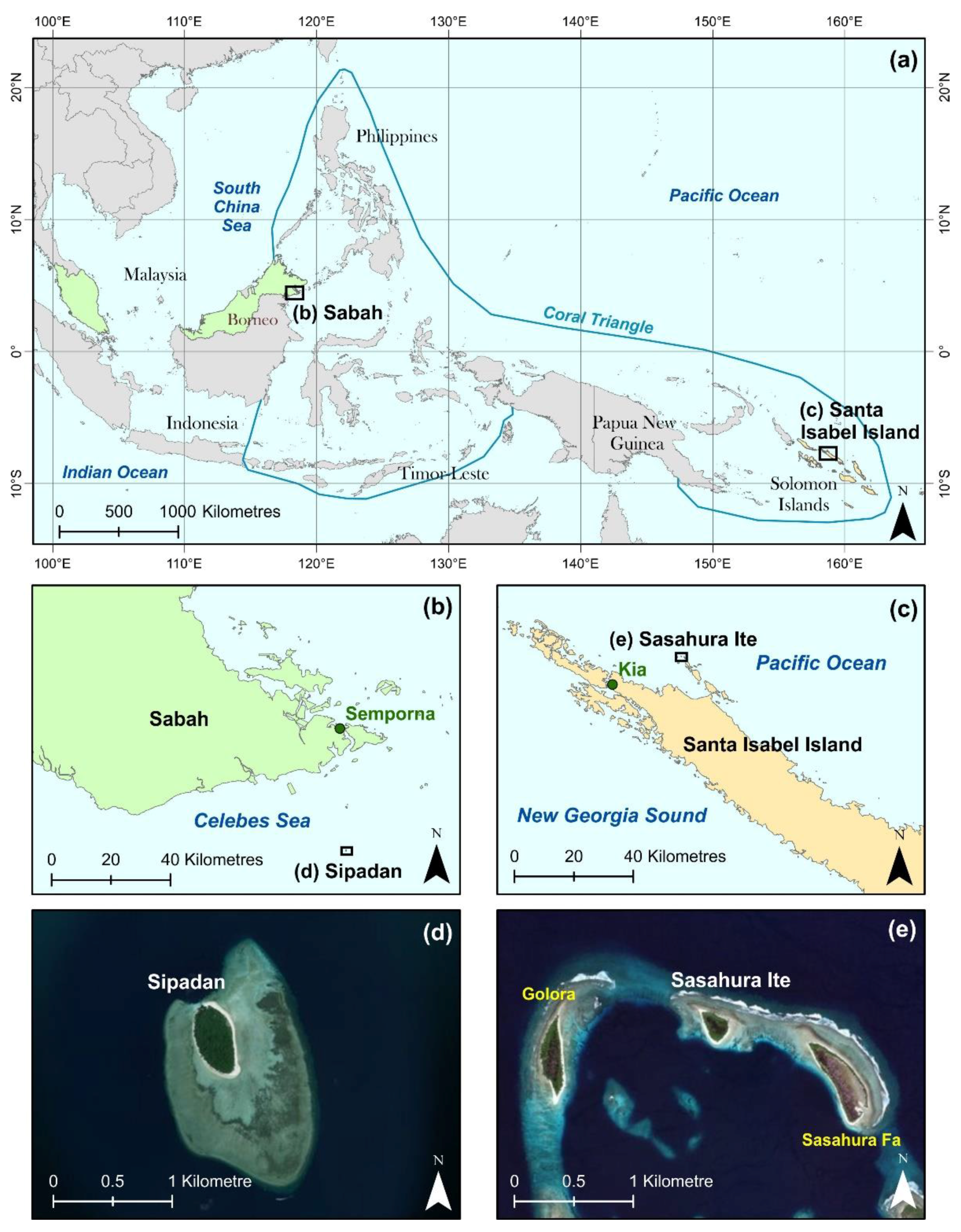
The two islands analysed in this study, Sipadan and Sasahura Ite, are located at the far western and eastern reaches of the Coral Triangle, respectively, in the western Pacific Ocean (
Figure 1a). This biogeographic region is considered a global hotspot for marine biodiversity and has the highest species richness of scleractinian corals in the world, a large number of endemic species, and many reef islands [
37,
38]. Compared to the Indian and Pacific Oceans, relatively few studies of reef-island geomorphology have been conducted in the Coral Triangle. These include an analysis by Mann and Westphal [
39] of shoreline change on Takú Atoll, Papua New Guinea, the study by Albert et al. [
40] using historical aerial photography from the Solomon Islands (including Sasahura Ite), and the description by Kench and Mann [
38] of islands in the Spermonde Archipelago (Indonesia).
A desktop review of available satellite imagery indicated that both Sipadan and Sasahura Ite are relatively undisturbed reef islands of a scale suitable for survey by UAV, and analysis of historic aerial photography demonstrated shoreline mobility over past decades [
40]. These islands were, therefore, chosen as case studies for this analysis of reef-island change.
2.1. Sipadan Island
Sipadan is located off the southeastern coast of Sabah Province on the island of Borneo, Malaysia, within the tropical Celebes Sea (latitude 4.115°N, longitude 118.629°E;
Figure 1b). The island accumulated on top of the limestone cap of an extinct volcanic seamount [
41]. Sipadan is ovate in shape, covers an area of approximately 0.18 km
2, and is located on the northwestern side of a reef platform that has an area of approximately 1.7 km
2 (
Figure 1d). Apart from several buildings and a small jetty on the northern side of the island, Sipadan is densely vegetated and largely undeveloped. Sipadan previously had a larger number of buildings and other infrastructure to service the scuba diving and tourism industries; however, many buildings were demolished following its gazettal as a Marine Park in 2004. Sipadan and its unique terrestrial and marine biodiversity are currently managed by Sabah Parks [
42].
Climate in Sabah is influenced by the northeast and southwest monsoons, with the highest rainfall typically falling during the northeast monsoon from November to May. The southeast monsoon occurs from May to November, which is considered the dry season. Cooler currents typically flow from the South China Sea towards Sabah during the northeast monsoon. Sipadan typically experiences the strongest winds from the south and southeast, has a spring tidal range of approximately 1.5 m, and wave heights of approximately 0.5 m are common [
43,
44].
2.2. Sasahura Ite Island
Sasahura Ite Island is located off the northwestern coast of Santa Isabel Island, Isabel Province, Solomon Islands (latitude 7.467°S, longitude 158.644°E;
Figure 1c). The Solomon Islands are subject to tectonic deformation due to the convergence of the Pacific Plate, Solomon Arc block and Australian Plate [
45], although Isabel Province is considered less active than other areas [
40]. Sasahura Ite is one of a series of islands that are aligned along a barrier reef that runs roughly parallel to the island of Santa Isabel. The triangular island covers an area of approximately 0.05 km
2 and is located between the islands of Golora and Sasahura Fa on the northern side of a shallow U-shaped reef platform (
Figure 1e). Sasahura Ite is uninhabited but is visited periodically by local landowners who collect food from the island (eggs of the Melanesian Megapode,
Megapodius eremitaode) and fish the surrounding waters. The centre of the island is dominated by a large, swampy depression that is partially colonised by mangroves.
Situated in the tropical zone of the western Pacific, Isabel Province experiences a distinctly seasonal wind and wave climate [
46]. The dry season (May to October) is dominated by southeasterly tradewinds and low to moderate wave energy, whereas the wet season (November to April) is characterised by northerly and northwesterly winds and larger swell. The tides are semi-diurnal with an approximate spring tidal range of 1.5 m, as recorded by a temporary tide logger deployed at the site from November 2017 to July 2018.
2.3. Data Collection
Fieldwork on Sipadan was conducted in February 2016 (topographic surveys only) and October–November 2017 (topographic and UAV surveys). Fieldwork in Isabel Province was undertaken in November 2017 and October 2018 (topographic and UAV surveys on both occasions).
Topographic surveys were completed using a Leica Sprinter 150 Optical Level at low tide (instrument accuracy: 1.5 mm). On Sipadan, seven beach profiles were surveyed from temporary benchmarks near the vegetation line (markers placed by the Sabah Parks Authority or permanent features such as signboards and huts) to the base of the beach. As there are no built features on Sasahura Ite, five profile locations were selected at different beach orientations, and surveyed from the vegetation line to as far below the water line as practical. A position along the exposed beach on each profile was recorded using a handheld Trimble GeoXH 2008 GPS; the distance from the start of the profile to the GPS position was recorded so that the profile could later be digitised. Repeat topographic surveys used the same temporary benchmarks (Sipadan) or locations found by GPS and photo records of the original starting points (Sasahura Ite).
On Sasahura Ite, profile elevations were reduced to mean sea level (MSL), a conventionally used vertical datum, by measuring the elevation of the water level relative to each profile and recording the time of survey; these were then referenced to MSL, which was estimated from data recorded by a temporarily installed tide gauge (HOBO U20L Water Level Logger) [
47]. The
z elevations recorded by the Trimble GeoXH 2008 GPS were used to reduce the Sipadan topographic profiles to MSL.
To prepare for the UAV surveys (DJI Phantom 4 Standard, camera model FC330 3.61 mm, 12 megapixels, 1/2.3” CMOS sensor), flights were planned in the Map Pilot for DJI Application with 75% frontlap and 75% sidelap (
Table 1). The flight altitudes were set at 120 m and the survey areas covered the islands and adjacent reef platforms. Prior to the UAV surveys, temporary GCPs (size: 42 × 60 cm) were placed around Sipadan and Sasahura Ite and their positions recorded using the Trimble GeoXH 2008 GPS (
xyz coordinates were recorded for Sipadan;
xy coordinates for Sasahura Ite). On Sasahura Ite, the height of the GCPs above the water level was also surveyed and reduced to MSL, as described above. The UAV was then launched following the pre-prepared flight plans, returning home multiple times to allow for battery changes. All flights were conducted as close to low tide as possible.
2.4. Data Analysis
The Trimble GeoXH GPS files for the topographic profile positions and GCP positions were differentially code and carrier post-processed using the Trimble GPS Pathfinder Pro software and the Receiver Independent Exchange Format (RINEX) data from the nearest observation station. For Sipadan, this was Tawau, Sabah, approximately 80 km to the west (data sourced from the Department of Survey and Mapping, Malaysia), and, for Sasahura Ite, this was Honiara, Guadalcanal, approximately 260 km to the southeast (data sourced from Geoscience Australia).
The estimated xyz accuracy of the post-processed GPS files for Sipadan was 0.27 m (vertical datum: MSL), while the estimated xy accuracy for Sasahura Ite was 0.50 m in 2017 and 0.44 m in 2018. The estimated accuracy of the vertical datum (z elevations) on Sasahura Ite was calculated conservatively as 0.2 m to account for the survey instrument accuracy (0.0015 m), uncertainty associated with surveying the water level (estimated at 0.15 m), and root-mean-square error (RMSE) of the tide gauge measurements around a fitted tidal curve (0.02 m).
The UAV imagery was imported into Agisoft Photoscan version 1.4.3. Following photo alignment, markers were placed onto the GCPs visible in the imagery, and the corresponding
xyz coordinates (WGS84) were imported. The sparse point clouds were optimised according to the placement of the markers; then, dense point clouds, orthomosaics, and DSMs were generated. The DSMs were constructed from the point clouds using inverse distance weighting (IDW) interpolation. The accuracy of the DSMs was assessed against the topographic profiles, and it was found that the best fit was obtained by retaining the default marker accuracy value of 0.005 m during the sparse cloud optimization (although it should be noted that the specific GPS accuracy value is typically recommended at this step) [
30]. Selected UAV flight and processing parameters are provided in
Table 1.
2.4.1. DSM Accuracy Assessment
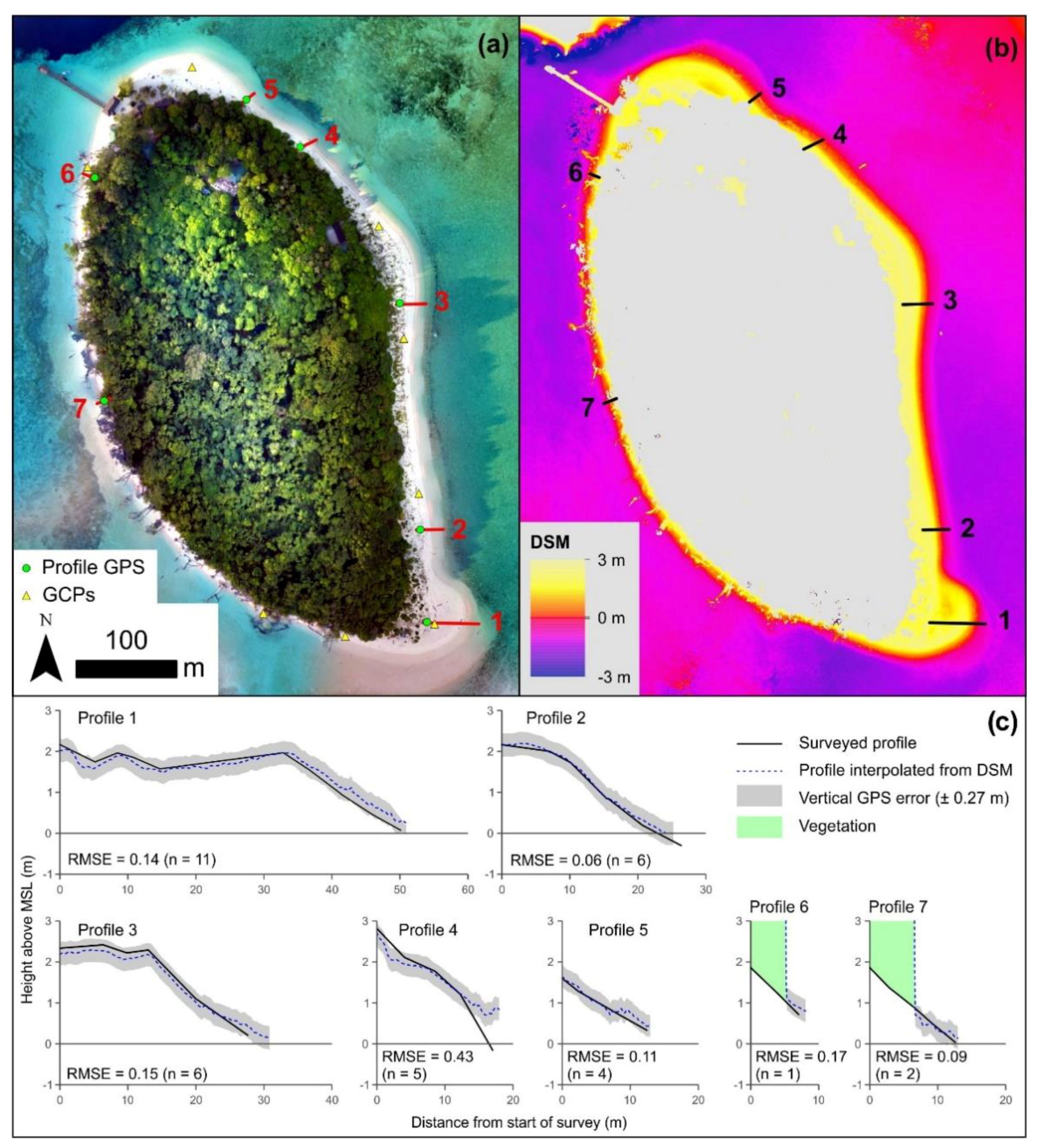
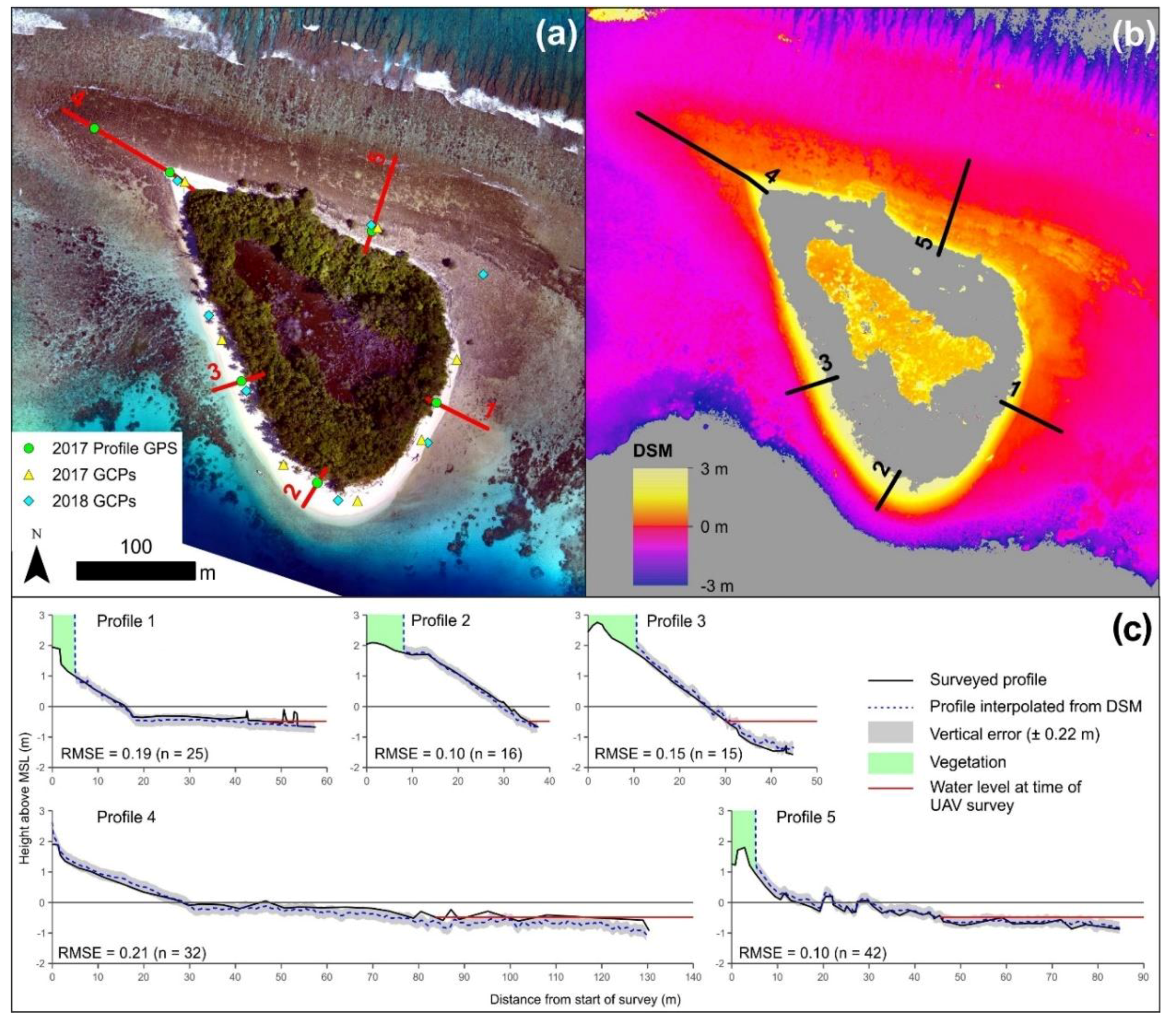
The accuracy of the DSMs was assessed by comparing them against the in situ topographic profiles. The 2017 DSMs and orthomosaics were imported into ArcMap 10.1. Polylines corresponding to the surveyed topographic profiles were drawn over the orthomosaics using the GPS positions and known profile lengths. The DSM surfaces were then interpolated onto the polylines using the Interpolate Shape tool in ArcToolbox, and the DSM-derived profiles were exported. These profiles were then plotted against the surveyed topographic profiles. The elevations corresponding to each point along the topographic profiles were extracted from the DSM-derived profiles. The extracted DSM elevations were then subtracted from the elevations of the corresponding topographic profile points and used to calculate the RMSE as an indication of the closeness of fit. Sections of the topographic profiles that were obstructed by vegetation on the DSMs were excluded from this analysis.
2.4.2. Planimetric vs. Volumetric Change Assessment
When choosing a shoreline proxy for assessing planimetric shoreline change, it is necessary to consider the type of change being assessed and the relevant temporal scale [
15,
48]. The base of beach (BB) was chosen for this study given the short study interval and specific focus on beach dynamics. BB on reef islands (sometimes also referred to as toe of beach; ToB) is indicated by a change in substrate and beach slope where the beach meets the reef flat [
39], and is identifiable on orthomosaics and high-resolution satellite imagery. Furthermore, BB position can change markedly on seasonal and annual timescales [
12], which are applicable to this study. Many longer-term studies of reef-island change use the edge of vegetation line (VL) as the shoreline proxy, as it may be more indicative of long-term island position and is easier to detect on lower-resolution satellite imagery and historic aerial photography [
40,
49,
50].
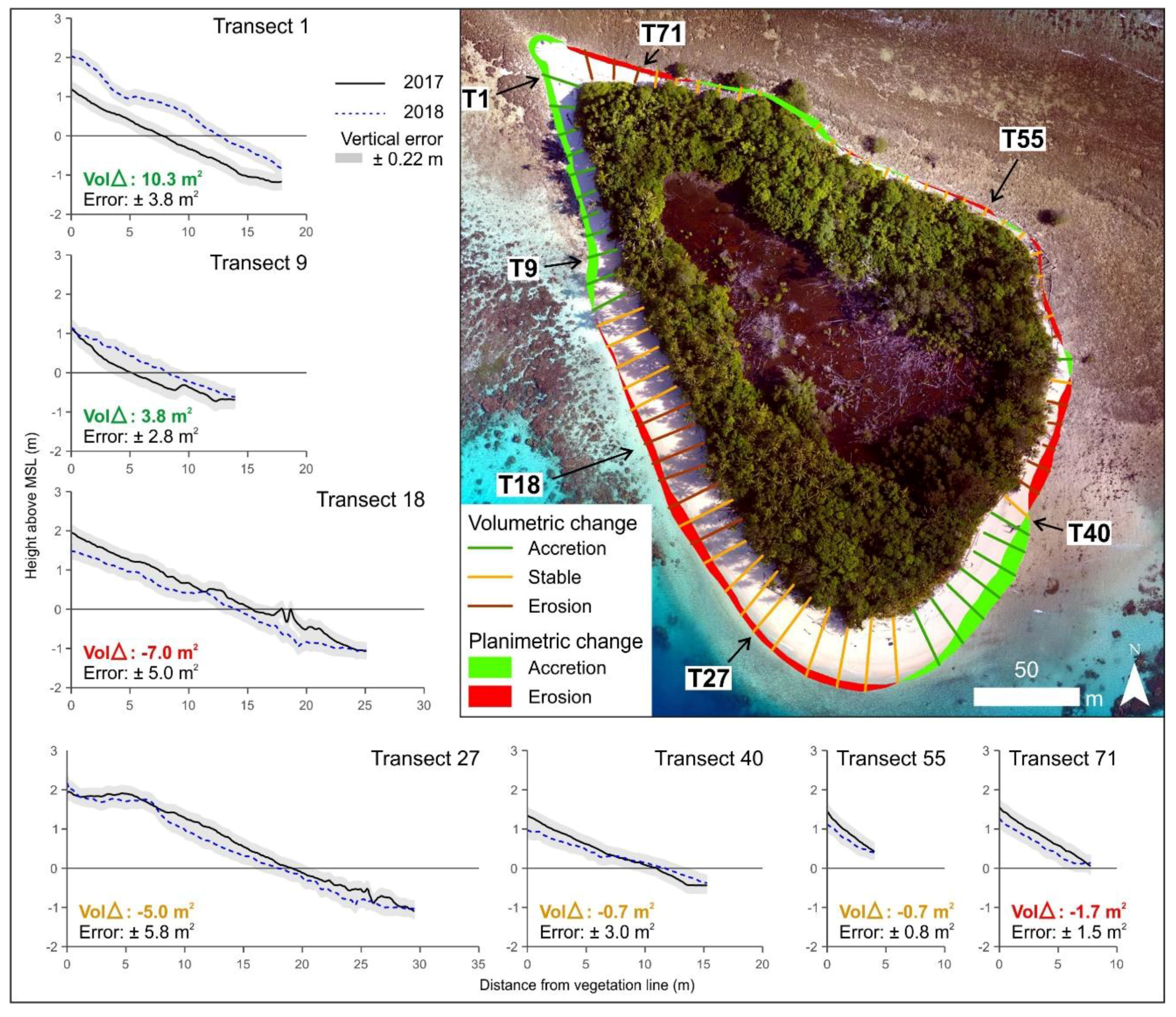
The positions of the BB on Sipadan and Sasahura Ite were, therefore, digitised from each UAV-derived orthomosaic via visual identification at a scale of 1:200. As no UAV survey was conducted at Sipadan in February 2016, a RapidEye-3 satellite image (Date: 27 January 2016) was used instead. The VL was also digitised as a baseline, as it did not observably change on Sipadan or Sasahura Ite within the study period. The distance between the VL and BB was then calculated as a measure of beach planimetric change. This was conducted at each of the seven surveyed topographic profile positions on Sipadan. Due to the availability of two UAV-derived datasets on Sasahura Ite, greater spatial coverage could be achieved by measuring planimetric change around the entire island, rather than just at the sites of the five surveyed profiles. For this purpose, 75 transects were cast around Sasahura Ite at a spacing of 10 m, and planimetric change was calculated at all transects except two where the BB was obscured by vegetation. The total beach area was also calculated for each dataset.
To determine the change in volume, the area under the repeat beach profiles from each survey period was calculated for Sipadan; horizontal baselines were established below the lowest surveyed point (the absolute elevation of this baseline is irrelevant, as only relative change was analysed). For Sasahura Ite, beach profiles were interpolated from both the 2017 and 2018 DSMs under the 73 viable transects and change in area under the curve calculated. The error associated with the volumetric change measurements was calculated as the length of the profile (VL to furthest BB line) multiplied by the vertical error term. This was estimated as 0.1 m for Sipadan, to conservatively incorporate the survey instrument accuracy (0.0015 mm) and estimated error associated with surveying a sandy surface (0.05 m). The vertical error term was estimated as 0.22 m at Sasahura Ite to account for the vertical accuracy of the surveyed GCPs (0.2 m; see
Section 2.4), plus the GCP
z error reported during the SfM processing (0.023 m; see
Table 1).
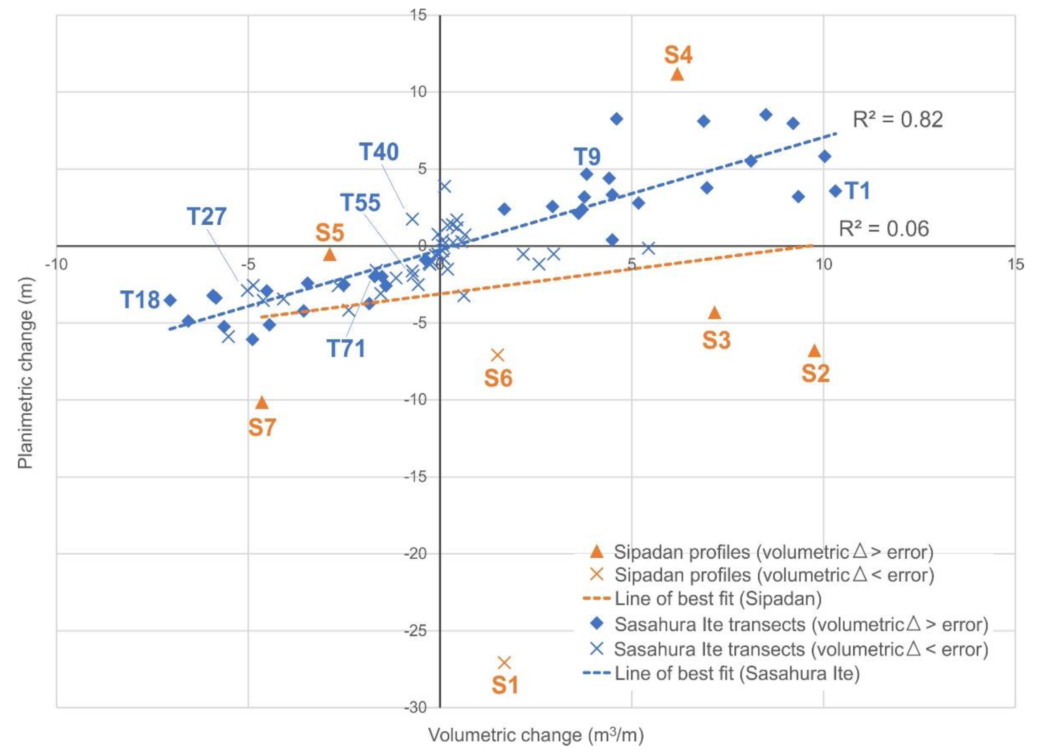
The volumetric change for each profile and transect was then assessed. Volumetric change was plotted against the planimetric change to analyse the strength of correlation. The coefficient of determination (R2) was then calculated using statistical regression (the proportion of variation in shoreline movement explained by the variation in beach volumetric change). Transects where the calculated error exceeded the volumetric change were excluded from the correlation calculation.
2.5. Comment on Error in the Analysis
There are a range of sources of error in this analysis that particularly affect how the volumetric change results should be interpreted. Firstly, the uncertainty associated with the topographic profile and GCP positions recorded by the Trimble GeoXH 2008 GPS was of similar scale to some of the volumetric changes that were detected. Positional error could be reduced in future studies by using a real-time kinematic (RTK) base station and rover to attain higher accuracy. Secondly, a greater number of GCPs, including a second set that could be used for validation of the DSM, would have been beneficial. In addition, greater image overlap (i.e., 90% frontlap and at least 60% sidelap) and alteration of the processing parameters could improve the accuracy of output data [
30,
34]. As a result, there may be additional sources of error that were not expressly considered in this analysis.
While in some cases the calculated error may be greater than the change detected, the results below demonstrate that it is possible to gain detailed planimetric and volumetric data using UAVs and develop workflows for the quantitative assessment of reef-island change. Of note, researchers working in remote environments often have limited time within which to undertake fieldwork and may be affected by sub-optimal conditions, at times resulting in trade-offs between the quality and quantity of data collected.
4. Discussion
UAV-derived orthomosaics and DSMs are valuable tools for assessing geomorphic changes [
23,
24,
30]. For reef-island beaches, where sub-metre changes in elevation can be significant for landform stability, the ability to model small-scale volumetric changes is particularly important. This study found that the high-resolution UAV-derived DSMs generated for Sipadan and Sasahura Ite aligned closely with the corresponding in situ topographic profiles (average RMSE = 0.16 m). Within the constraints of relevant errors and uncertainties, significantly greater spatial coverage of three-dimensional information can be achieved using UAVs in a reduced timeframe compared to traditional surveying methods, and for considerably less expense than alternative remote sensing options [
11]. UAV-derived DSMs also facilitate analysis and interpretation of three-dimensional beach morphology and island behaviour that is not possible using planimetric methods.
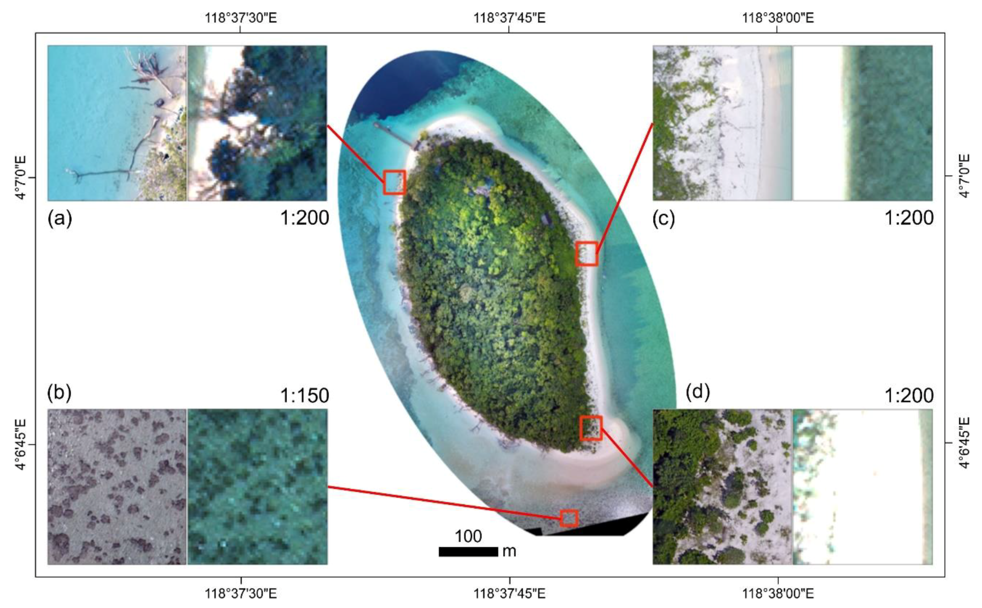
There are also clear advantages to using UAV-derived orthomosaics instead of satellite imagery in terms of image resolution; the orthomosaics generated in this study had pixel resolutions of approximately 5 cm (
Table 1), compared to satellite imagery such as Worldview-2, which has a pixel resolution of 46 cm. Furthermore, pixel saturation of highly reflective surfaces can affect the visibility of features in satellite imagery. Shoreline proxies such as the base of the beach (and, therefore, total beach area) can be determined with greater confidence on UAV-derived orthomosaics. In addition, smaller features on islands and reefs, such as vegetation patterns, fallen trees, and individual corals, can be readily identified (
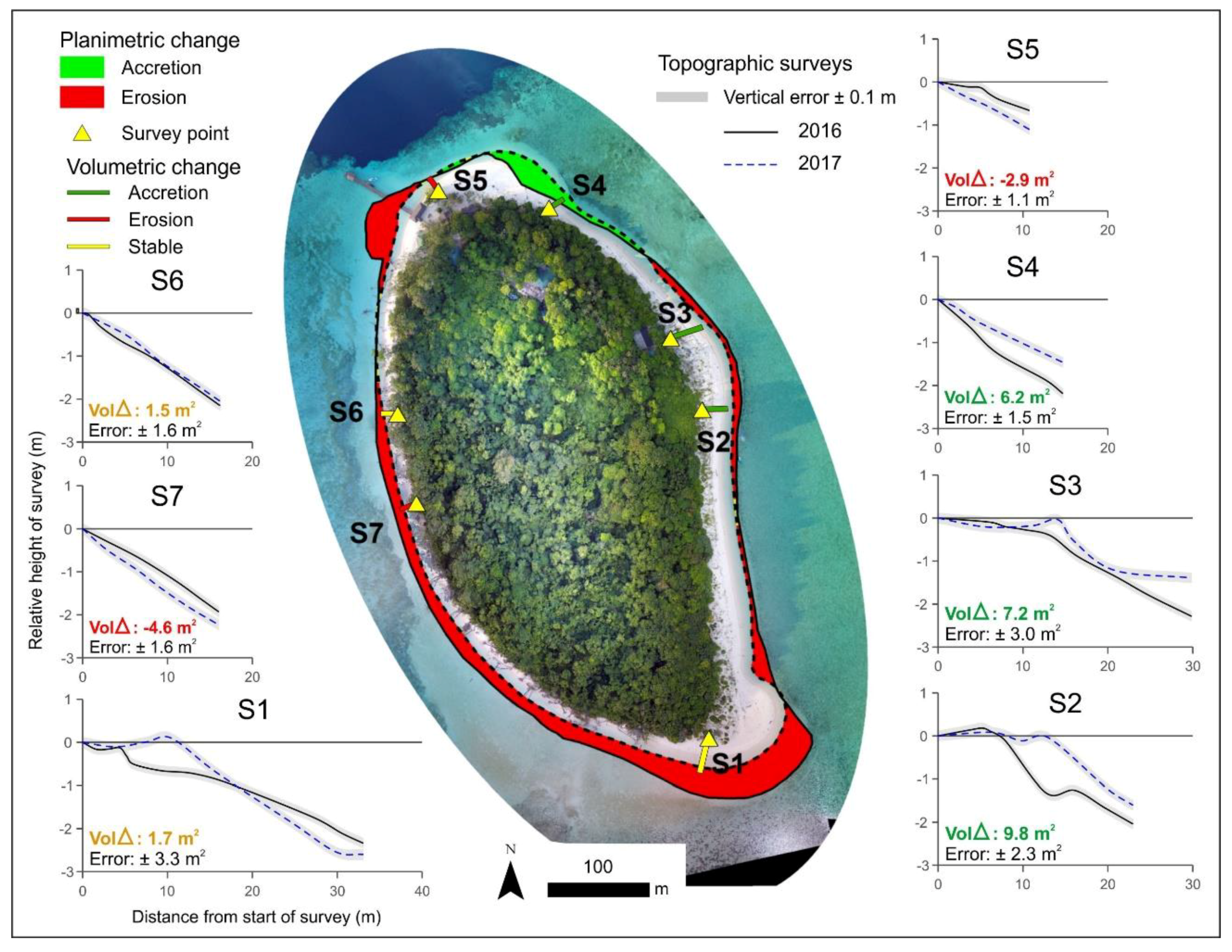
Figure 7). This enables planimetric changes to not only be more accurately measured, but other geomorphic processes can also be inferred. For example, as seen on Sipadan, the narrow beach and fallen trees on the western side indicate an eroding shoreline, whereas the wider beach adjacent to younger successional vegetation on the eastern side indicates an accretional shoreline. These observations can supplement and contextualise quantitative analyses of shoreline change.
Sipadan and Sasahura Ite exhibited different patterns of change within the study periods; volumetric change and planimetric change did not correlate on Sipadan, while, on Sasahura Ite, volumetric change was a moderately strong indicator of planimetric change (R2 = 0.82). Such a situation may be explained by different shoreline behaviours at the sites.
Beaches do not always maintain the same slope and shape as they erode or accrete, as more complicated topographic transformations can take place [
51]; this appears to be the case on Sipadan. The western shoreline eroded, while, on the eastern shoreline, the accumulation of a beach berm corresponded with planimetric narrowing of the beach (
Figure 4, S1 to S3). This provides an example of a potentially common situation in which volumetric increases can be interpreted planimetrically as erosion. Therefore, analyses of reef-island change that rely solely on planimetric datasets may not always tell the full story.
The observations of both erosion and accretion around the island periphery at Sasahura Ite further demonstrate the dynamic nature of reef-island shorelines; areas that eroded during the study period were offset by equivalent areas of accretion. Adjacent sections of coastline appear to be connected via processes of alongshore sediment transport, while the overall island remains in a state of dynamic equilibrium. Such dynamic equilibria were observed in the Maldives and on other reef islands in response to seasonal climate oscillations [
9,
12]. Unlike on Sipadan, changes to beach morphology on Sasahura Ite did not often involve significant reshaping of the three-dimensional profile; as such, planimetric change and volumetric change were correlated. However, on approximately half of the transects on Sasahura Ite (38 of 73), the calculated uncertainty exceeded the volumetric change; these profiles were, therefore, considered stable and were excluded from the correlation analysis.
Separating the “signal” (the geomorphic changes) from the “noise” (the error associated with the techniques for measuring these changes) is a common analytical challenge when evaluating shoreline changes [
28,
29]. Fundamentally, the magnitude of change observed must be greater than the cumulative margin of error of the techniques employed to measure that change [
28]. Maximum certainty in shoreline change evaluation requires large shoreline fluctuations measured using high-accuracy techniques. Furthermore, datasets must be collected on a spatial and temporal scale relevant to the processes being analysed, i.e., shoreline response to seasonal fluctuation or climatic oscillations.
The high resolution of UAV-derived orthomosaics enables planimetric shoreline change to be measured where the magnitude of change (the signal) exceeds the GPS accuracy plus the pixel resolution (the noise); this represents a considerable improvement to the methods previously utilised for shoreline change detection [
11,
28]. There are additional sources of uncertainty associated with the volumetric change measurements (as outlined in
Section 2.5); as such, these results should be interpreted with caution. However, even where there is greater uncertainty in the absolute volume of change, analysis of three-dimensional beach morphology can still be highly valuable for interpreting patterns of shoreline behaviour.
The methods applied for assessing volumetric change in this study could be further refined and improved. The
xyz accuracy of the GPS positions could be increased using additional equipment (i.e., an RTK base station and rover), although it is noted that many reef islands are located in countries that have limited facilities (including spatial correction networks) for collecting reliable spatial data [
52]. Furthermore, fixed features (such as prominent fossil corals that are exposed at low tide) could be used as GCPs where possible, and the vertical uncertainty associated with GCP
z elevations could be reduced by surveying all points to a fixed benchmark. In addition, data analysis techniques could be refined; for example, the datasets could be aligned in three dimensions using point cloud analysis software (such as CloudCompare with the M3C2 plugin) so that relative volumetric change can be determined [
23].
While some limitations were identified, this study demonstrated that adopting a multifaceted approach to the assessment of reef-island change using UAV-derived orthomosaics and DSMs can support a more comprehensive understanding of shoreline dynamics and greater insight into relevant geomorphic processes. However, despite the added value of these orthomosaics and DSMs, logistical considerations will limit the number of remote reef islands on which repeat UAV datasets can be collected. As such, studies of large numbers of reef islands are still likely to rely on planimetric assessments of change using repeat satellite imagery. It would be advantageous if high-resolution planimetric and volumetric studies of selected reef islands are conducted alongside lower-resolution remotely sensed planimetric analyses to contextualise the patterns of change observed in the wider sample.
Significance and Future Research
This study presents an initial assessment of UAV-derived planimetric and volumetric change on reef islands. While the short interval between the surveys in this study and magnitude of errors are such that the changes observed may not be representative of longer-term trends, continued refinement and application of these methods will provide valuable insights into patterns of reef-island change. Furthermore, modelling (and, where possible, measuring) wave, wind, and tidal processes that act on reef-island shorelines, in combination with repeat high-resolution mapping, may enable links to be drawn between observed morphologies and geomorphic processes.
Advancements in UAV technology will also enable data to be collected more efficiently, and with greater accuracy and spatial coverage. New UAV models, such as the DJI Phantom 4 RTK, integrate high-accuracy differential GPS positioning that reduces the number of GCPs required and, thus, the time-consuming process of laying out and surveying them (although a validation dataset of GCPs is still required to assess the accuracy of outputs). Furthermore, as different types of UAV-borne sensors (such as LiDAR and multispectral sensors) become lighter and more affordable, researchers who are currently restricted by UAV weight regulations will be able to collect a greater range of spatial information. This may include access to more detailed digital surface elevation information below the canopy on reef islands and further into the nearshore zone to better quantify entire island morphologies. Depositional features under the canopy, such as storm ridges and terraces, could be detected, and the bathymetry surrounding the island could be mapped; this would enable the volume of the whole island to be calculated, and provide additional insights into reef island morphodynamics.
Understanding how reef-island beaches respond to changing environmental conditions will be particularly important given the projected impacts of climate change over coming decades. Higher-intensity storms, sea-level rise, ocean acidification, and the changing species composition of coral reefs (which supply islands with sediment) are all predicted to have implications for reef-island stability into the future [
53,
54,
55]. Further investigation into the likely effects of these processes will be essential for informing sustainable adaptation for communities that reside on or utilise resources from reef islands.

 ,
, 


