Article

New Generalized Jacobi Galerkin Operational Matrices of Derivatives: An Algorithm for Solving Multi-Term Variable-Order Time-Fractional Diffusion-Wave Equations

by
Hany Mostafa Ahmed
Department of Mathematics, Faculty of Technology and Education, Helwan University, Cairo 11281, Egypt
Fractal Fract. 2024, 8(1), 68; https://doi.org/10.3390/fractalfract8010068
Submission received: 14 December 2023 / Revised: 11 January 2024 / Accepted: 15 January 2024 / Published: 18 January 2024
(This article belongs to the Special Issue Feature Papers for Numerical and Computational Methods Section)

Abstract

:
The current study discusses a novel approach for numerically solving MTVO-TFDWEs under various conditions, such as IBCs and DBCs. It uses a class of GSJPs that satisfy the given conditions (IBCs or DBCs). One of the important parts of our method is establishing OMs for Ods and VOFDs of GSJPs. The second part is using the SCM by utilizing these OMs. This algorithm enables the extraction of precision and efficacy in numerical solutions. We provide theoretical assurances of the treatment’s efficacy by validating its convergent and error investigations. Four examples are offered to clarify the approach’s practicability and precision; in each one, the IBCs and DBCs are considered. The findings are compared to those of preceding studies, verifying that our treatment is more effective and precise than that of its competitors.

1. Introduction

Fractional calculus has emerged as a subject of great interest among researchers from diverse fields in recent decades. The universal perspective that fractional operators offer for comprehending system dynamics is what primarily motivates this interest. Fractional derivatives offer a more precise and comprehensive description of various physical phenomena compared to traditional integer-order derivatives [1,2,3,4]. Consequently, there exists a wide range of definitions for fractional differentiation in the literature (for further details, refer to [5,6,7]). A list of abbreviations used in the paper is given in Abbreviations Section.
Researchers have made worthy progress in the field of fractional calculus, emphasizing the extension of the framework to encompass VOFDs. This extension facilitates an understanding of diverse dynamic systems. The authors in [8] conducted a specific study in which they investigated the characteristics of VOFD operators [9,10].
VOFC is a strong framework that obtains the nonlocal properties of different systems very well [11,12,13,14,15,16,17,18]. For instance, in study [19], the utilization of VOFD operators enabled the modeling of the microscopic structure of materials. As shown in an additional publication [20], continuum elasticity also made use of the Riesz–Caputo fractional derivative of space-dependent order. In [21], the authors recommend using collocation and tau spectral techniques to solve the time-fractional heat equation numerically. Studies [22,23] specifically focused on understanding and analyzing how the fractional order, which characterizes the system’s dynamics, evolves over time and influences its viscoelastic properties. By examining the time-dependent changes in the fractional order, valuable insights were gained into the complex behavior of such systems. Overall, VOFC has proven to be a valuable tool in engineering mechanics, providing a versatile approach to accurately describe and analyze a wide range of dynamic systems.
The pursuit of analytical solutions for FDEs poses a significant challenge, often necessitating reliance on numerical approximations. As a result, various numerical techniques have addressed the complexities associated with FDEs, enabling researchers to effectively tackle problems that would otherwise be challenging to solve analytically. Previous research has witnessed the utilization of a variety of approaches to create numerical solutions for FDEs through the use of both orthogonal and non-orthogonal polynomials. There are a number of papers [24,25,26,27,28,29,30] that talk about different OMs of JPs and some of their special cases. These papers use different spectral methods by utilizing these OMs to solve different kinds of DEs and FDEs numerically, subject to different kinds of IBCs. Additionally, researchers in [31,32,33,34,35,36] follow the same methodology to solve VOFDEs numerically. Additionally, in [37,38], Bernstein polynomials were employed to approximate solutions for FDEs. Another notable contribution in [39] proposed a numerical scheme based on Fourier analysis for solving FDEs. Furthermore, finite difference approximations were discussed in [40] as a means to construct numerical schemes for FDEs. In [41], the author uses a class of modified JPs to introduce a novel method for numerically solving MTVO-FDEs with initial conditions.
Many researchers [42,43,44] have shown that JPs have properties that make them very useful for solving different kinds of DEs, especially when spectral methods are used. Some of these properties are that they are orthogonal, have exponential accuracy, and have two parameters that allow us to shape approximate solutions in different ways. These inherent properties of JPs make them highly suitable for effectively solving a wide range of diverse problems encountered in various fields of study.
It is worth noting that a significant class of fractional partial differential equations that has received considerable attention in recent years is the TFDWE. This equation arises from the classical diffusion-wave equation by replacing the second-order time derivative term with a fractional derivative of order 1 < α < 2 [45]. The TFDWE describes important physical effects seen in many different types of systems, such as colloidal, amorphous, glassy, and porous materials, as well as dielectrics and semiconductors, comb structures, polymers, random and disordered media, biological systems, and geophysical and geological processes (see [46] and references therein).
Furthermore, it is worth mentioning that the TFDWE serves as an accurate model for many universal electromagnetic, acoustic, and mechanical responses [47,48]. A single TFDWE may not be able to fully describe the underlying processes in some real-life situations. This is why an MTFDWE was created, as shown in [46,49]. This MTFDWE formulation offers a more comprehensive representation of complex systems and their dynamic behavior, allowing for more accurate modeling of the underlying processes.
We considered the general form of MTVO-TFDE in our investigation as follows:
D 0 c t ν ( x , t ) + j = 1 m ϱ j D 0 c t ν j ( x , t ) y ( x , t ) + ϱ y t ( x , t ) = κ y x x ( x , t ) + g ( x , t ) , ( x , t ) [ 0 , ] × [ 0 , T ] ,
subject to the IBCs:
y ( x , 0 ) = f 1 ( x ) , y t ( x , 0 ) = f 2 ( x ) , y ( 0 , t ) = f 3 ( t ) , y ( , t ) = f 4 ( t ) ,
or the DBCs:
y ( x , 0 ) = f 1 ( x ) , y ( x , T ) = f 2 ( x ) , y ( 0 , t ) = f 3 ( t ) , y ( , t ) = f 4 ( t ) ,
where ϱ j ( j = 1 , 2 , , m , m N ) , ϱ 0  and κ > 0 are constants; 1 < ν 1 ( x , t ) < ν 2 ( x , t ) < < ν m ( x , t ) < ν ( x , t ) 2 holds; f 0 ( x ) , f 1 ( x ) , f 2 ( x ) , f 3 ( t ) , f 4 ( t ) and g ( x , t ) are given functions; and D 0 c t ν ( x , t ) a n d D 0 c t ν j ( x , t ) ( i = 1 , 2 , , m ) are the VOFDs defined in the Caputo sense, as given in Section 2. The significance and difficulty of proving the existence, unicity, and dependency of parameters should be emphasized. The significance of determination of ν and ν j in (1) is evident in theory and practice due to the strong relationship between them and the heterogeneity and associated physical features of media [50]. For instance, in the situation of a single term case, Cheng et al. [51] first demonstrated the uniqueness of ν using the boundary condition data that were provided.
We present a new Galerkin OM for Ods and new OMs for VOFDs of GSJPs in the sense of Caputo. This was made in order to find a new way to solve the problem shown by (1) and the conditions (2) or (3). These operational matrices are specifically tailored for the basis vectors of GSJPs. Leveraging these OMs, we have established a powerful tool that enables the accurate computation of numerical solutions using the SCM to solve a wide range of MTVO-TFDEs. This novel method opens up new ways to solve this type of FDE numerically and more effectively.
To summarize, the main article’s contributions are as follows:
(i)
We introduce two classes of GSJPs to satisfy the given IBCs and DBCs (see Section 3.2).
(ii)
We establish Galerkin OMs for the Ods and for VOFDs of the introduced GSJPs in the sense of Caputo (see Section 4 and Section 5).
(iii)
We address the presented MTVO-TFDE using the proposed GSJPs and their constructed OMs in conjunction with the SCM (see Section 6).
(iv)
We present a study of convergence and error analysis for the numerical solution obtained through the proposed scheme (see Section 7).
The paper has the following outline: Section 2 provides comprehensive coverage of the needed concepts of VOFC. Section 3 highlights the necessary attributes of JPs and GSJPs. Section 4 and Section 5 emphasize the development of new Galerkin OMs for Ods and VOFDs of GSJPs. These OMs are intended to address Equation (1) when IBCs (2) or DBCs (3) are considered. Section 6 explores the selection of newly generated OMs in the SCM to address the aforementioned issue. Section 7 analyzes convergence and error estimation. Section 8 includes four examples to clarify the approach’s practicability and precision, and the findings are compared to those of preceding studies, verifying that our treatment is more effective and precise than its competitors. Finally, Section 9 summarizes the key outcomes, implications derived from our investigation, and the scope of future work.

2. Basic Definition of Caputo VOFDs

This section serves to introduce and discuss important definitions and necessary assets that lay the groundwork for the development of our proposed technique. These tools are crucial building blocks that provide the necessary foundation for effectively handling the MTVO-TFDE under consideration.
Definition 1
([39,45]). Suppose h ( x , t ) is a twice differentiable function. The Caputo derivative operator with the variable-order ν ( x , t ) is defined as:
D 0 c t ν ( x , t ) h ( x , t ) = 1 Γ ( 2 ν ( x , t ) ) 0 t ( t τ ) 1 ν ( x , t ) 2 h ( x , τ ) τ 2 d τ , 1 < ν ( x , t ) < 2 , h t t ( x , t ) , ν ( x , t ) = 2 .
The Caputo VOFD exhibits the characteristics:
D 0 c t ν ( x , t ) ( λ 1 h 1 ( t ) + λ 2 h 2 ( t ) ) = λ 1 D 0 c t ν ( x , t ) h 1 ( t ) + λ 2 D 0 c t ν ( x , t ) h 2 ( t ) ,
D 0 c t ν ( x , t ) ( C ) = 0 , ( C is a constant ) ,
D 0 c t ν ( x , t ) t k = 0 , k = 0 , 1 , Γ ( k + 1 ) Γ ( k + 1 ν ( x , t ) ) t k ν ( x , t ) , k = 2 , 3 , .
Remark 1.
The reader who is interested may find several definitions and additional attributes of VOFDs in [4] (pp. 35–42).

3. An Overview of the Shifted JPs and Their Generalized Ones

Introducing the fundamental features of the JPs and their shifting form is the main objective of this section. Additionally, a group of GSJPs is introduced.

3.1. An Overview of the Shifted JPs

The orthogonal JPs, J n ( α ^ , β ^ ) ( x ) , α ^ , β ^ > 1 , satisfy the following relationship [52]:
1 1 w α ^ , β ^ ( x ) J n ( α ^ , β ^ ) ( x ) J m ( α ^ , β ^ ) ( x ) d x = 0 , m n , h n ( α ^ , β ^ ) , m = n ,
where w α ^ , β ^ ( x ) = ( 1 x ) α ^ ( 1 + x ) β ^ and h n ( α ^ , β ^ ) = 2 λ Γ ( n + α ^ + 1 ) Γ ( n + β ^ + 1 ) n ! ( 2 n + λ ) Γ ( n + λ ) ,   λ = α ^ + β ^ + 1 .
The shifted JPs, denoted as J , n ( α ^ , β ^ ) ( t ) = J n ( α ^ , β ^ ) ( 2 t / 1 ) , are in accordance with:
0 w α ^ , β ^ ( t ) J , n ( α ^ , β ^ ) ( t ) J , m ( α ^ , β ^ ) ( t ) d t = 0 , m n , 2 λ h n ( α ^ , β ^ ) , m = n ,
where w α ^ , β ^ ( t ) = ( t ) α ^ t β ^ .
The fundamental expansions that will be used in this paper are [53] (Section 11.3.4):
  • The power form representations of J , n ( α ^ , β ^ ) ( t ) are as follows:
    J , i ( α ^ , β ^ ) ( t ) = k = 0 i c k ( i ) t k = k = 0 i c ¯ k ( i ) ( t ) k ,
    where
    c k ( i ) = ( 1 ) i k Γ ( i + β ^ + 1 ) Γ ( i + k + λ ) k k ! ( i k ) ! Γ ( k + β ^ + 1 ) Γ ( i + λ ) and c ¯ k ( i ) = ( 1 ) k ( α ^ + 1 ) i ( λ + i ) k k k ! ( i k ) ! ( α ^ + 1 ) k .
  • Alternatively, the expressions for t k and ( t ) k in relation to J , r ( α ^ , β ^ ) ( t ) have the forms:
    t k = r = 0 k b r ( k ) J , r ( α ^ , β ^ ) ( t ) , a n d ( t ) k = r = 0 k b ¯ r ( k ) J , r ( α ^ , β ^ ) ( t ) ,
    where
    b r ( k ) = k k ! ( λ + 2 r ) Γ ( k + β ^ + 1 ) Γ ( r + λ ) ( k r ) ! Γ ( r + β ^ + 1 ) Γ ( k + r + λ + 1 ) a n d b ¯ r ( k ) = ( 2 j + λ ) k ( k ) j ( λ + 1 ) j 1 ( α ^ + 1 ) k ( α ^ + 1 ) j ( λ + 1 ) k ( k + λ + 1 ) j .

3.2. Introducing GSJPs

In this section, it is helpful to talk about two polynomials, { ϕ T , j ( α ^ , β ^ ) ( t ) } j 0 and { ψ , j ( α ^ , β ^ ) ( t ) } j 0 . These are needed to satisfy the homogeneous form of the given IBCs (2) and DBCs (3):
ϕ T , j ( α ^ , β ^ ) ( t ) = t 2 J T , j ( α ^ , β ^ ) ( t ) ,
ψ , j ( α ^ , β ^ ) ( t ) = t ( t ) J , j ( α ^ , β ^ ) ( t ) .
Subsequently, these polynomials satisfy the orthogonality relations as follows:
0 T w T α ^ , β ^ ( t ) t 4 ϕ T , i ( α ^ , β ^ ) ( t ) ϕ T , j ( α ^ , β ^ ) ( t ) d t = 0 , i j , T 2 λ h i ( α ^ , β ^ ) , i = j ,
0 w α ^ , β ^ ( t ) t 2 ( t ) 2 ψ , i ( α ^ , β ^ ) ( t ) ψ , j ( α ^ , β ^ ) ( t ) d t = 0 , i j , 2 λ h i ( α ^ , β ^ ) , i = j ,
where w ρ α ^ , β ^ ( t ) = ( ρ t ) α ^ t β ^ .

4. Two OMs for Ods and VOFDs of ϕ T , j ( α ^ , β ^ ) ( t )

In this part, we introduce two OMs related to ODEs and VOFDs of ϕ T , j ( α ^ , β ^ ) ( t ) . To facilitate this, we commence with Theorem 1:
Theorem 1
([41]). D ( t n J T , i ( α ^ , β ^ ) ( t ) ) for all i 0 can be computed as follows:
D ( t n J T , i ( α ^ , β ^ ) ( t ) ) = j = 0 i 1 θ i , j α ^ , β ^ ( n , T ) ( t n J T , i ( α ^ , β ^ ) ( t ) ) + ϵ n , i ( t ) ,
where ϵ n , i ( t ) = n i ! ( 1 ) i ( β ^ + 1 ) i t n 1 ,  and 
θ i , j α ^ , β ^ ( n , T ) = C i , j α ^ , β ^ r = 0 i j 1 ( 1 ) r ( j + n + r + 1 ) ( i + j + λ + 1 ) r r ! ( j + r + 1 ) ( j + r + β ^ + 1 ) Γ ( i j r ) Γ ( 2 j + r + λ + 1 ) ,
where
C i , j α ^ , β ^ = ( 1 ) i + j 1 ( λ + i ) ( β ^ + 1 ) i ( λ + 2 j ) Γ ( j + λ ) ( i + λ + 1 ) j T ( β ^ + 1 ) j .
Then, the two desired OMs of
Φ T , N ( α ^ , β ^ ) ( t ) = [ ϕ T , 0 ( α ^ , β ^ ) ( t ) , ϕ T , 1 ( α ^ , β ^ ) ( t ) , , ϕ T , N ( α ^ , β ^ ) ( t ) ] T
can be computed as follows:
Corollary 1
([41]). The general derivative of Φ T , N ( α ^ , β ^ ) ( t ) has the form:
d m Φ T , N ( α ^ , β ^ ) ( t ) d t m = G m Φ T , N ( α ^ , β ^ ) ( t ) + η N ( m ) ( t ) ,
with η N ( m ) ( t ) = k = 0 m 1 G k ϵ N ( m k 1 ) ( t ) , where ϵ N ( t ) = ϵ 2 , 0 ( t ) , ϵ 2 , 1 ( t ) , , ϵ 2 , N ( t ) T   a n d   G = ( g i , j ) 0 i , j N ,
g i , j = θ i , j α ^ , β ^ ( 2 , T ) , i > j , 0 , otherwise .
Theorem 2.
D ν ( x , t ) ϕ T , i ( α ^ , β ^ ) ( t ) for all i 0 , has the form:
D 0 c t ν ( x , t ) ϕ T , i ( α ^ , β ^ ) ( t ) = t ν ( x , t ) j = 0 i Θ i , j ( ν ( x , t ) ) ϕ T , j ( α ^ , β ^ ) ( t ) ,
which leads to:
D 0 c t ν ( x , t ) Φ T , N ( α ^ , β ^ ) ( t ) = t ν ( x , t ) D ( ν ( x , t ) ) Φ T , N ( α ^ , β ^ ) ( t ) ,
where D ( ν ( x , t ) ) = ( d i , j ( ν ( x , t ) ) ) is a matrix of order ( N + 1 ) × ( N + 1 ) , which can be expressed explicitly as:
Θ 0 , 0 ( ν ( x , t ) ) 0 0 Θ 1 , 0 ( ν ( x , t ) ) Θ 1 , 1 ( ν ( x , t ) ) 0 0 Θ i , 0 ( ν ( x , t ) ) Θ i , i ( ν ( x , t ) ) 0 0 0 Θ N , 0 ( ν ( x , t ) ) Θ N , N ( ν ( x , t ) ) ,
where
d i , j ( ν ( x , t ) ) = Θ i , j ( ν ( x , t ) ) , i j , 0 , otherwise ,
and
Θ i , j ( ν ( x , t ) ) = ( 1 ) i j ( j + 2 ) ! Γ ( i + β ^ + 1 ) Γ ( j + λ ) Γ ( i + j + λ ) ( i j ) ! Γ ( j + β ^ + 1 ) Γ ( 2 j + λ ) Γ ( i + λ ) Γ ( j ν ( x , t ) + 3 ) × 3 F 2 j i , j + 3 , i + j + λ 2 j + λ + 1 , j ν ( x , t ) + 3 ; 1 .
Proof. 
By considering (7) and applying (6b), we obtain:
D 0 c t ν ( x , t ) ϕ T , i ( α ^ , β ^ ) ( t ) = t 2 ν ( x , t ) k = 0 i c k ( i ) Γ ( k + 3 ) Γ ( k ν ( x , t ) + 3 ) t k .
By utilizing (9), expanding and collecting similar terms, and using useful computational formulae of the Pochhammer symbol and the Gamma function (see [54] (p. 758)), it is possible to convert (24) to (19), which is represented as follows:
D 0 c t ν ( x , t ) ϕ T , i ( α ^ , β ^ ) ( t ) = t ν ( x , t ) [ Θ i , 0 ( ν ( x , t ) ) , Θ i , 1 ( ν ( x , t ) ) , , Θ i , i ( ν ( x , t ) ) , 0 , , 0 ] Φ T , N ( α ^ , β ^ ) ( t ) ,
and this representation enables us to declare that (20) is proved and that the theorem is completely proved.    □
As an application of Theorem 2, for  N = 4 , α ^ = β ^ = 1 / 2 , and  ν ( x , t ) = x t , the OM D ( ν ( x , t ) ) has the form:
D ( ν ( x , t ) ) = 2 Γ ( 3 t x ) 0 0 0 0 t x Γ ( 4 t x ) 6 Γ ( 4 t x ) 0 0 0 3 t x ( t x + 2 ) 4 Γ ( 5 t x ) 27 t x 2 Γ ( 5 t x ) 24 Γ ( 5 t x ) 0 0 5 t x ( t x + 1 ) ( t x + 5 ) 8 Γ ( 6 t x ) 45 t x ( t x + 1 ) 2 Γ ( 6 t x ) 100 t x Γ ( 6 t x ) 120 Γ ( 6 t x ) 0 35 t x ( t x + 1 ) ( t x + 2 ) ( t x + 9 ) 64 Γ ( 7 t x ) 525 t x ( t x + 1 ) ( t x + 2 ) 16 Γ ( 7 t x ) 175 t x ( 3 t x + 2 ) 2 Γ ( 7 t x ) 735 t x Γ ( 7 t x ) 720 Γ ( 7 t x ) 5 × 5 .

5. Two OMs for Ods and VOFDs of ψ , i ( α ^ , β ^ ) ( t )

In this part, we establish two OMs for Ods and VOFDs of ψ , i ( α ^ , β ^ ) ( t ) . In order to achieve this, we commence by proving the subsequent lemma:
Lemma 1.
The polynomials t J , i ( α ^ , β ^ ) ( t ) , i 0 have the following representation:
t J , i ( α ^ , β ^ ) ( t ) = j = 0 i 1 Υ i , j α ^ , β ^ ( ) ψ , j ( α ^ , β ^ ) ( t ) + ( α ^ + 1 ) i i ! t ,
where
Υ i , j α ^ , β ^ = Γ ( i + α ^ + 1 ) Γ ( j + λ ) Γ ( i + j + λ + 1 ) ( j + 1 ) Γ ( i j ) Γ ( j + α ^ + 2 ) Γ ( i + λ ) Γ ( 2 j + λ ) 4 F 3 i + j + 1 , j + 1 , α ^ + j + 1 , λ + i + j + 1 j + 2 , α ^ + j + 2 , λ + 2 j + 1 ; 1 .
Proof. 
We have
J , i ( α ^ , β ^ ) ( t ) = ( t ) J , i ( α ^ , β ^ ) ( t ) J , i ( α ^ , β ^ ) ( ) t + J , i ( α ^ , β ^ ) ( ) .
In view of (7) and (9), we obtain:
J , i ( α ^ , β ^ ) ( t ) J , i ( α ^ , β ^ ) ( ) t = k = 0 i 1 c ¯ k + 1 ( i ) ( t ) k = k = 0 i 1 c ¯ k + 1 ( i ) r = 0 k b ¯ r ( k ) J , i ( α ^ , β ^ ) ( t ) ,
consequently, through expansion, the accumulation of similar terms, and using useful computational formulae of the Pochhammer symbol and the Gamma function (see [54] (p. 758)), it becomes evident that:
J , i ( α ^ , β ^ ) ( t ) J , i ( α ^ , β ^ ) ( ) t = j = 0 i 1 Υ i , j α ^ , β ^ ( ) J , j ( α ^ , β ^ ) ( t ) .
Substitution of (31) and J , i ( α ^ , β ^ ) ( ) = ( α ^ + 1 ) i i ! into (29) leads to (27), and then the lemma is proved completely.    □
Theorem 3.
D ψ , i ( α ^ , β ^ ) ( t ) , for all i 0 , has the form:
D ψ , i ( α ^ , β ^ ) ( t ) = j = 0 i 1 Ω i , j α ^ , β ^ ( ) ψ , j ( α ^ , β ^ ) ( t ) + ϑ , i ( t ) ,
where ϑ , i ( t ) = 1 i ! ( ( 1 ) i ( t ) ( β ^ + 1 ) i t ( α ^ + 1 ) i ) , and
Ω i , j α ^ , β ^ ( ) = θ i , j α ^ , β ^ ( 1 , ) + Υ i , j α ^ , β ^ ( ) ,
Proof. 
We have
D ψ , i ( α ^ , β ^ ) ( t ) = ( t ) D ( t J , i ( α ^ , β ^ ) ( t ) ) t J , i ( α ^ , β ^ ) ( t ) .
Using Theorem 1 and Lemma 1 leads to (32), and the proof of the theorem is complete.    □
Then, the desired two OMs of
Ψ , N ( α ^ , β ^ ) ( t ) = [ ψ , 0 ( α ^ , β ^ ) ( t ) , ψ , 1 ( α ^ , β ^ ) ( t ) , , ψ , N ( α ^ , β ^ ) ( t ) ] T
can be computed as follows:
Corollary 2.
The general derivative of Ψ , N ( α ^ , β ^ ) ( t ) is expressed as:
d m Ψ , N ( α ^ , β ^ ) ( t ) d t m = H m Ψ , N ( α ^ , β ^ ) ( t ) + ξ , N ( m ) ( t ) ,
with ξ , N ( m ) ( t ) = k = 0 m 1 H k ϑ , N ( m k 1 ) ( t ) , where ϑ , N ( t ) = ϑ , 0 ( t ) , ϑ , 1 ( t ) , , ϑ , N ( t ) T a n d H = h i , j 0 i , j N ,
h i , j = Ω i , j α ^ , β ^ ( ) , i > j , 0 , otherwise .
Theorem 4.
D 0 c t ν ( x , t ) ψ , i ( α ^ , β ^ ) ( t ) for all i 0 , has the expression
D 0 c t ν ( x , t ) ψ , i ( α ^ , β ^ ) ( t ) = t ν ( x , t ) j = 0 i Λ i , j ( ν ( x , t ) ) ψ , j ( α ^ , β ^ ) ( t ) + ε , i ( x , t ) ,
which leads to
D 0 c t ν ( x , t ) Ψ , N ( α ^ , β ^ ) ( t ) = t ν ( x , t ) D ^ ( ν ( x , t ) ) Ψ , N ( α ^ , β ^ ) ( t ) + ε , N ( x , t ) ,
where ε , N ( x , t ) = ε , 0 ( x , t ) , ε , 1 ( x , t ) , , ε , N ( x , t ) T and D ^ ( ν ( x , t ) ) = ( d ^ i , j ( ν ( x , t ) ) ) is a matrix of order ( N + 1 ) × ( N + 1 ) , which can be expressed explicitly as:
Λ 0 , 0 ( ν ( x , t ) ) 0 0 Λ 1 , 0 ( ν ( x , t ) ) Λ 1 , 1 ( ν ( x , t ) ) 0 0 Λ i , 0 ( ν ( x , t ) ) Λ i , i ( ν ( x , t ) ) 0 0 0 Λ N , 0 ( ν ( x , t ) ) Λ N , N ( ν ( x , t ) ) ,
where the matrix elements are defined as follows:
d ^ i , j ( ν ( x , t ) ) = Λ i , j ( ν ( x , t ) ) , i j , 0 , otherwise ,
and the coefficients Λ i , j ( ν ( x , t ) ) have the form
Λ i , j ( ν ( x , t ) ) = Ξ i , j ( 1 ) ( ν ( x , t ) ) + Ξ i , j ( 2 ) ( ν ( x , t ) ) ,
where
Ξ i , j ( 1 ) ( ν ( x , t ) ) = ( j + 2 ) ! ( 1 ) i j ( λ ) j ( λ ) i + j ( β ^ + 1 ) i ( i j ) ! ( λ ) i ( λ ) 2 j ( β ^ + 1 ) j Γ ( j ν ( x , t ) + 3 ) × 3 F 2 i + j , j + 3 , i + j + λ 2 j + λ + 1 , 3 + j ν ( x , t ) ; 1 ,
Ξ i , j ( 2 ) ( ν ( x , t ) ) = ( 1 ) i + 1 ( 2 j + λ ) ( β ^ + 1 ) i ( λ ) j ν ( x , t ) ( β ^ + 1 ) j ( λ ) i r = j i ( 1 ) r ( r + 2 ) r ! ( λ + 1 ) i + r ( β ^ + r + 1 ) ( i r 1 ) ! ( r j ) ! ( λ + 1 ) j + r Γ ( r ν ( x , t ) + 4 ) × 4 F 3 1 , r + 3 , i + r + 1 , i + λ + r + 1 r + 2 , β ^ + r + 2 , 4 + r ν ( x , t ) ; 1 ,
and the functions ε , i ( x , t ) have the form
ε , i ( x , t ) = ( 1 ) i + 1 ( β ^ + 1 ) i ν ( x , t ) t i ! Γ ( 3 ν ) 3 F 2 i , i + λ , 2 β ^ + 1 , 3 ν ( x , t ) ; 1 .
Proof. 
By considering (7) and applying (6b), it is easy to see that
D 0 c t ν ( x , t ) ψ , i ( α ^ , β ^ ) ( t ) = t ν ( x , t ) s = 0 i c k ( i ) Γ ( s + 2 ) t s + 1 Γ ( s + 3 ν ( x , t ) ) ( ( s + 2 ) ( t ) ν ( x , t ) ) ,
which may be expressed as:
D 0 c t ν ( x , t ) ψ , i ( α ^ , β ^ ) ( t ) = t ν ( x , t ) 1 + 2 + 3 ,
where
1 = s = 0 i c s ( i ) Γ ( s + 3 ) Γ ( s + 3 ν ( x , t ) ) ( t ( t ) ) t s ,
2 = s = 0 i c s ( i ) Γ ( s + 2 ) ν ( x , t ) Γ ( s + 3 ν ( x , t ) ) t ( s t s ) ,
and
3 = s = 0 i c s ( i ) Γ ( s + 2 ) ν ( x , t ) Γ ( s + 3 ν ( x , t ) ) s + 1 t .
Using (9), through expansion, the accumulation of similar terms, and some algebraic manipulation (see [54] (p. 758)), it becomes evident that
1 = j = 0 i Ξ i , j ( 1 ) ( ν ( x , t ) ) ψ , j ( α ^ , β ^ ) ( t ) .
Also, substitution of the form c s ( i ) in (49)—after some simple algebraic manipulation—gives
3 = ε , i ( x , t ) .
Now, it remains that we show that
2 = j = 0 i Ξ i , j ( 2 ) ( ν ( x , t ) ) ψ , j ( α ^ , β ^ ) ( t ) .
Using s t s = s 1 ( t ) k = 0 s 1 k t k and c i + 1 ( i ) = 0 —after some algebraic manipulation—leads to:
2 = s = 0 i c s + 1 ( i ) s + 1 Γ ( s + 3 ) ν ( x , t ) Γ ( s + 4 ν ( x , t ) ) t ( t ) k = 0 s k t k .
By expanding and collecting similar terms, we obtain:
2 = j = 0 i B i , j t ( t ) t j ,
where
B i , j = s = j i c s + 1 ( i ) s j + 1 Γ ( s + 3 ) ν ( x , t ) Γ ( s + 4 ν ( x , t ) ) .
Again, using (9), expanding and collecting similar terms leads to:
2 = j = 0 i r = j i B i , r b j ( r ) ψ , j ( α ^ , β ^ ) ( t ) .
Using the expressions of c s + 1 ( i ) and b j ( r ) after some algebraic manipulation leads to:
r = j i B i , r b j ( r ) = Ξ i , j ( 2 ) ( ν ( x , t ) ) ,
then
2 = j = 0 i Ξ i , j ( 2 ) ( ν ( x , t ) ) ψ , j ( α ^ , β ^ ) ( t ) .
In view of Equations (46), (50), (51), and (58), the proof of (37) is complete, which can be expressed as follows:
D 0 c t ν ( x , t ) ψ , i ( α ^ , β ^ ) ( t ) = t ν ( x , t ) [ Λ i , 0 ( ν ( x , t ) ) , Λ i , 1 ( ν ( x , t ) ) , , Λ i , i ( ν ( x , t ) ) , 0 , , 0 ] Ψ , N ( α ^ , β ^ ) ( t ) + ε , i ( x , t ) ;
this gives (38), and the theorem is completely proved.    □
As an application of Corollary 2 and Theorem 4, for  N = 4 , α ^ = β ^ = 1 / 2 , and  ν ( x , t ) = x t , the OMs H and D ^ ( ν ( x , t ) ) have the forms:
H = 1 0 0 0 0 0 6 0 0 0 0 3 2 12 0 0 0 10 5 2 50 3 0 0 35 16 315 16 35 12 21 0 5 × 5 ,
and
D ^ ( ν ( x , t ) ) = 2 Γ ( 3 t x ) 0 0 0 0 5 t x Γ ( 4 t x ) 6 Γ ( 4 t x ) 0 0 0 3 t x ( 13 t x + 14 ) 4 Γ ( 5 t x ) 63 t x 2 Γ ( 5 t x ) 24 Γ ( 5 t x ) 0 0 5 t x ( 5 t x ( 5 t x + 18 ) + 41 ) 8 Γ ( 6 t x ) 15 t x ( 13 t x + 9 ) 2 Γ ( 6 t x ) 180 t x Γ ( 6 t x ) 120 Γ ( 6 t x ) 0 35 t x ( t x ( t x ( 41 t x + 312 ) + 481 ) + 186 ) 64 Γ ( 7 t x ) 105 t x ( 7 t x ( 5 t x + 11 ) + 38 ) 16 Γ ( 7 t x ) 35 t x ( 43 t x + 22 ) 2 Γ ( 7 t x ) 1155 t x Γ ( 7 t x ) 720 Γ ( 7 t x ) 5 × 5 .

6. Numerical Handling for MTVO-TFDWEs Subject to IBCs (2) or DBCs (3)

OMs from Section 4 and Section 5 are used in this section to find numerical solutions for MTVO-TFDWEs (1) when IBCs (2) or DBCs (3) are present.

6.1. Homogeneous IBCs and DBCs

Suppose that the IBCs (2) or the DBCs (3) are homogeneous; that is, f 1 ( x ) = f 2 ( x ) = f 3 ( t ) = f 4 ( t ) = 0 . We can consider
y ( x , t ) y N ( x , t ) = i = 0 N j = 0 N a i , j ψ , i ( α ^ , β ^ ) ( x ) ϕ T , j ( α ^ , β ^ ) ( t ) = Ψ , N ( α ^ , β ^ ) ( x ) A Φ T , N ( α ^ , β ^ ) ( t )
in the case of IBCs, while in the case of DBCs, we have
y ( x , t ) y N ( x , t ) = i = 0 N j = 0 N a i , j ψ , i ( α ^ , β ^ ) ( x ) ψ , j ( α ^ , β ^ ) ( t ) = Ψ , N ( α ^ , β ^ ) ( x ) A Ψ T , N ( α ^ , β ^ ) ( t ) ,
where A = ( a i , j ) ( N + 1 ) × ( N + 1 ) is the unknown matrix.
Corollaries 1 and 2 and Theorems 2 and 4 allow us to approximate the derivatives of y ( x , t ) that appear in Equation (1) according to the conditions considered, IBCs/DBCs, as follows:
D 0 c t ν ( x , t ) y N ( x , t ) = i = 0 N j = 0 N a i , j ψ , i ( α ^ , β ^ ) ( x ) D 0 c t ν ( x , t ) ϕ T , j ( α ^ , β ^ ) ( t ) = t ν ( x , t ) Ψ , N ( α ^ , β ^ ) ( x ) A D ( ν ( x , t ) ) Φ T , N ( α ^ , β ^ ) ( t ) , for IBCs , i = 0 N j = 0 N a i , j ψ , i ( α ^ , β ^ ) ( x ) D 0 c t ν ( x , t ) ψ T , j ( α ^ , β ^ ) ( t ) = t ν ( x , t ) Ψ , N ( α ^ , β ^ ) ( x ) A ( D ^ ( ν ( x , t ) ) Ψ T , N ( α ^ , β ^ ) ( t ) + ε T , N ( x , t ) ) , for DBCs ,
D t y N ( x , t ) = i = 0 N j = 0 N a i , j ψ , i ( α ^ , β ^ ) ( x ) D t ϕ T , j ( α ^ , β ^ ) ( t ) = Ψ , N ( α ^ , β ^ ) ( x ) A ( G Φ T , N ( α ^ , β ^ ) ( t ) + η T , N ( 1 ) ( t ) ) , for IBCs , i = 0 N j = 0 N a i , j ψ , i ( α ^ , β ^ ) ( x ) D t ψ T , j ( α ^ , β ^ ) ( t ) = Ψ , N ( α ^ , β ^ ) ( x ) A ( H Ψ T , N ( α ^ , β ^ ) ( t ) + ξ T , N ( 1 ) ( t ) ) , for DBCs ,
and
D x x y N ( x , t ) = i = 0 N j = 0 N a i , j D x x ψ , i ( α ^ , β ^ ) ( x ) ϕ T , j ( α ^ , β ^ ) ( t ) = ( H 2 Ψ , N ( α ^ , β ^ ) ( x ) + ξ , N ( 2 ) ( x ) ) A Φ T , N ( α ^ , β ^ ) ( t ) , for IBCs , i = 0 N j = 0 N a i , j D x x ψ , i ( α ^ , β ^ ) ( x ) ψ T , j ( α ^ , β ^ ) ( t ) = ( H 2 Ψ , N ( α ^ , β ^ ) ( x ) + ξ , N ( 2 ) ( x ) ) A Ψ T , N ( α ^ , β ^ ) ( t ) , for DBCs .
In this method, using the approximations (62)–(66) allows one to write the residual of Equation (1) as:
R N ( x , t ) = D 0 c t ν ( x , t ) + j = 1 m ϱ j D 0 c t ν j ( x , t ) y N ( x , t ) + ϱ D t y N ( x , t ) κ D x x y N ( x , t ) g ( x , t ) .
Now, we suggest a spectral approach called GSJCOPMM to obtain an approximate solution for (1) under the IBCs (2) or DBCs (3) (with f 1 ( x ) = f 2 ( x ) = f 3 ( t ) = f 4 ( t ) = 0 ). The collocation points x i , t i ( 0 i N ) are chosen to be either the zeros of J , N + 1 ( α ^ , β ^ ) ( x ) and J T , N + 1 ( α ^ , β ^ ) ( t ) or the points x i = ( i + 1 ) N + 2 and t i = T ( j + 1 ) N + 2 , i , j = 0 , 1 , , N , respectively. Therefore, we have
R N ( x i , t j ) = 0 , i , j = 0 , 1 , , N .
We can compute a i , j (where i , j = 0 , 1 , , N ) by using the right solver to work through a set of ( N + 1 ) 2 Equation (68). Achieving the target numerical solution relies heavily on these coefficients.

6.2. Non-Homogeneous IBCs and DBCs

Changing Equation (1) along with the non-homogeneous conditions (2) or (3) into a similar form with homogeneous conditions is an important part of creating the proposed algorithm. The following transformation accomplishes this change:
u ( x , t ) = y ( x , t ) q ( x , t ) , q ( x , t ) = q 1 ( x , t ) + q 2 ( x , t ) ,
where the two functions q 1 ( x , t ) and q 2 ( x , t ) are defined as follows:
  • In the Case of IBCs:
q 1 ( x , t ) = 1 [ ( x ) ( f 3 ( t ) f 2 ( 0 ) t f 3 ( 0 ) ) + x ( f 4 ( t ) f 2 ( ) t f 4 ( 0 ) ) ] , q 2 ( x , t ) = f 1 ( x ) + f 2 ( x ) t . }
  • In the Case of DBCs:
q 1 ( x , t ) = 1 T [ ( x ) ( T f 3 ( t ) f 2 ( 0 ) t f 1 ( 0 ) ( T t ) ) f 1 ( ) x ( T t ) f 2 ( ) x t + T x f 4 ( t ) ] , q 2 ( x , t ) = 1 T [ ( T t ) f 1 ( x ) + t f 2 ( x ) ] . }
As a result, the current issue may be simplified by solving the following updated equation:
D 0 c t ν ( x , t ) + j = 1 m ϱ j D 0 c t ν j ( x , t ) u N ( x , t ) + ϱ D t u N ( x , t ) = κ D x x u N ( x , t ) + g ˜ ( x , t ) ,
where
g ˜ ( x , t ) = g ( x , t ) + κ D x x D 0 c t ν ( x , t ) j = 1 m ϱ j D 0 c t ν j ( x , t ) ϱ D t q ( x , t ) ,
subject to the homogeneous IBCs
u ( x , 0 ) = u t ( x , 0 ) = u ( 0 , t ) = u ( , t ) = 0 ,
or the homogeneous DBCs
u ( x , 0 ) = u ( x , 0 ) = u ( 0 , t ) = u ( , t ) = 0 .
Then,
y N ( x , t ) = u N ( x , t ) + q ( x , t ) .
Remark 2.
Section 8 explains the algorithm that was used to solve various numerical examples. An Intel® Core™ i9-10850 CPU running at 3.60 GHz, with 10 cores and 20 logical processors and 64.0 GB RAM, was used to do the calculations on a computer system equipped with Mathematica 13.3.1.0 with GSJCOPMM, and the following algorithmic steps may be described to solve the MTVO-TFDWE (Algorithms 1 and 2):
Algorithm 1 GSJCOPMM algorithm to solve (1) subject to IBCs.
Stage 1.Given α ^ , β ^ , , T , N , ν ( x , t ) , ν i ( x , t ) and f j , i = 1 , 2 , , m , j = 1 , 2 , 3 , 4 .
Stage 2.Define the basis ψ , i ( α ^ , β ^ ) ( x ) and ϕ T , j ( α ^ , β ^ ) ( t ) , the matrices
A , G , H , η N ( m ) ( t ) , ξ , N ( m ) ( x ) , Ψ , N ( α ^ , β ^ ) ( x ) Φ T , N ( α ^ , β ^ ) ( t ) ,
and calculate the elements of matrices   G , H 2 , η N ( 1 ) ( t ) , ξ , N ( 2 ) ( x ) D ( ν ( x , t ) ) , and
D ( ν i ( x , t ) ) , i = 1 , 2 , , m .
Stage 3.Calculate the matrices:
1. Ψ , N ( α ^ , β ^ ) ( x ) A Φ T , N ( α ^ , β ^ ) ( t ) ,
2. Ψ , N ( α ^ , β ^ ) ( x ) A ( G Φ T , N ( α ^ , β ^ ) ( t ) + η N ( 1 ) ( t ) ) ,
3. ( H 2 Ψ , N ( α ^ , β ^ ) ( x ) + ξ , N ( 2 ) ( x ) ) A Φ T , N ( α ^ , β ^ ) ( t ) ,
4. Ψ , N ( α ^ , β ^ ) ( x ) A D ( ν ( x , t ) ) Φ T , N ( α ^ , β ^ ) ( t ) ,
5. Ψ , N ( α ^ , β ^ ) ( x ) A D ( ν i ( x , t ) ) Φ T , N ( α ^ , β ^ ) ( t ) , i = 0 , 1 , , m .
Stage 4.Define R N ( x , t ) as in Equation (67).
Stage 5.List R N ( x i , t j ) = 0 , i , j = 0 , 1 , , N , defined in Equation (68).
Stage 6.Use Mathematica’s built-in numerical solver to solve the system obtained in [Output 5].
Stage 6.Calculate y N ( x , t ) defined in Equation (62) (Homogeneous IBCs).
Stage 7.Calculate q ( x , t ) and y N ( x , t ) defined in Equation (75) (Non-homogeneous IBCs).
Algorithm 2 GSJCOPMM algorithm to solve (1) subject to DBCs.
Stage 1.Given α ^ , β ^ , , T , N , ν ( x , t ) , ν i ( x , t ) and f j , i = 1 , 2 , , m , j = 1 , 2 , 3 , 4 .
Stage 2.Define the basis ψ , i ( α ^ , β ^ ) ( x ) , the matrices A , H , ε T , N ( x , t ) , ξ , N ( m ) ( t ) , Ψ , N ( α ^ , β ^ ) ( x ) , and calculate the elements
of matrices  H 2 , ξ T , N ( 1 ) ( t ) , ξ , N ( 2 ) ( x ) D ^ ( ν ( x , t ) ) , and D ^ ( ν i ( x , t ) ) , i = 1 , 2 , , m .
Stage 3.Calculate the matrices:
1. Ψ , N ( α ^ , β ^ ) ( x ) A Ψ T , N ( α ^ , β ^ ) ( t ) ,
2. Ψ , N ( α ^ , β ^ ) ( x ) A ( H Ψ T , N ( α ^ , β ^ ) ( t ) + ξ T , N ( 1 ) ( t ) ) ,
3. ( H 2 Ψ , N ( α ^ , β ^ ) ( x ) + ξ , N ( 2 ) ( x ) ) A Ψ T , N ( α ^ , β ^ ) ( t ) ,
4. Ψ , N ( α ^ , β ^ ) ( x ) A ( D ^ ( ν ( x , t ) ) Ψ T , N ( α ^ , β ^ ) ( t ) + ε T , N ( x , t ) ) ,
5. Ψ , N ( α ^ , β ^ ) ( x ) A ( D ^ ( ν i ( x , t ) ) Ψ T , N ( α ^ , β ^ ) ( t ) + ε T , N ( x , t ) ) , i = 0 , 1 , , m .
Stage 4.Define R N ( x , t ) as in Equation (67).
Stage 5.List R N ( x i , t j ) = 0 , i , j = 0 , 1 , , N , defined in Equation (68).
Stage 6.Use Mathematica’s built-in numerical solver to solve the system obtained in [Output 5].
Stage 6.Calculate y N ( x , t ) defined in Equation (62) (Homogeneous DBCs).
Stage 7.Calculate q ( x , t ) and y N ( x , t ) defined in Equation (75) (Non-homogeneous DBCs).

7. Convergence and Error Analysis

Here, we look at the suggested method’s convergence and error estimations. The space S N , defined as follows, is our primary area of interest,
S N = S p a n { ψ , i ( α ^ , β ^ ) ( x ) ϕ T , j ( α ^ , β ^ ) ( t ) : i , j = 0 , 1 , , N } , for IBCs , S p a n { ψ , i ( α ^ , β ^ ) ( x ) ψ T , j ( α ^ , β ^ ) ( t ) : i , j = 0 , 1 , , N } , for DBCs .
Additionally, the error between y ( x , t ) and its approximation y N ( x , t ) can be defined by
E N ( x , t ) = y ( x , t ) y N ( x , t ) .
The numerical scheme’s error is examined in the paper via the use of the L norm error estimation
E N = y y N = m a x ( x , t ) I | y ( x , t ) y N ( x , t ) | , I = [ 0 , ] × [ 0 , T ] .
In the following, Theorem 5 discusses the error estimate when the solution satisfies IBCs, while Theorem 6 discusses it when DBCs are considered.
Theorem 5.
Assume that y ( x , t ) = t 2 x ( x ) υ ( x , t ) and that y N ( x , t ) has the expression (62) and represents the best possible approximation (BPA) for y ( x , t ) out of S N . Then,
E N 1 4 ( T ) 2 W q , N ( , T ) , q = m a x { α ^ , β ^ , 1 / 2 } < N + 1 ,
where
W q , N ( , T ) = K 1 2 λ e 4 N ( N + 1 ) q N 1 + K 2 T 2 λ e T 4 N ( N + 1 ) q N 1 + K 3 T 2 2 λ e 2 T 16 N ( N + 1 ) 2 ( q N 1 ) ,
where the constants K i , i = 1 , 2 , 3 , are defined as follows:
K 1 = m a x ( x , t ) I | N + 1 υ ( x , t ) x N + 1 | , K 2 = m a x ( x , t ) I | N + 1 υ ( x , t ) t N + 1 | , K 3 = m a x ( x , t ) I | 2 N + 2 υ ( x , t ) x N + 1 t N + 1 | .
Proof. 
Let υ N ( x , t ) be the interpolating polynomial for υ ( x , t ) at the points ( x i , t j ) , i , j = 0 , 1 , , N , where x i , ( 0 i N ) and t j , ( 0 j N ) are the roots of J , N + 1 ( α ^ , β ^ ) ( x ) and J T , N + 1 ( α ^ , β ^ ) ( t ) , respectively, such that N > q 1 . Then, the function υ ( x , t ) can be written as [55]:
υ ( x , t ) = υ N ( x , t ) + N + 1 υ ( η x , t ) x N + 1 ( N + 1 ) ! Q 1 ( x ) + N + 1 υ ( x , η t ) t N + 1 ( N + 1 ) ! Q 2 ( t ) 2 N + 2 υ ( η x , η t ) x N + 1 t N + 1 ( ( N + 1 ) ! ) 2 Q 1 ( x ) Q 2 ( t ) ,
where Q 1 ( x ) = i = 0 N ( x x i ) , Q 2 ( t ) = j = 0 N ( t t j ) , η x , η x [ 0 , ] , and η t , η t [ 0 , T ] .
This is to acquire that:
υ υ N K 1 N + 1 ( N + 1 ) ! c ˜ N J , N + 1 ( α ^ , β ^ ) ( x ) + K 2 T N + 1 ( N + 1 ) ! c ˜ N J T , N + 1 ( α ^ , β ^ ) ( t ) + K 3 ( T ) N + 1 ( ( N + 1 ) ! ) 2 ( c ˜ N ) 2 J , N + 1 ( α ^ , β ^ ) ( x ) J T , N + 1 ( α ^ , β ^ ) ( t ) ,
where c ˜ N = N + 1 c N + 1 N + 1 = Γ ( 2 N + λ + 2 ) ( N + 1 ) ! Γ ( N + λ + 1 ) , and c N + 1 N + 1 is the leading coefficient of J , N + 1 ( α ^ , β ^ ) ( x ) .
Using the expression [52] (formula (7.32.2)), we derive:
J , N + 1 ( α ^ , β ^ ) ( N + 1 ) q ,
and thus the inequality (82) takes the form:
υ υ N K 1 N + 1 Γ ( N + λ + 1 ) ( N + 1 ) q Γ ( 2 N + λ + 2 ) + K 2 T N + 1 Γ ( N + λ + 1 ) ( N + 1 ) q Γ ( 2 N + λ + 2 ) + K 3 ( T ) N + 1 Γ 2 ( N + λ + 1 ) ( N + 1 ) 2 q Γ 2 ( 2 N + λ + 2 ) .
By utilizing results (see [56] (pp. 232–233)),
Γ ( m + λ ) = O ( m λ 1 m ! ) , ( 2 m ) ! = 1 π 4 m m ! Γ ( m + 1 / 2 ) , m ! = O 2 π m m e m ,
the inequality (84) takes the form:
υ υ N W q , N ( , T ) ,
where
W q , N ( , T ) = K 1 2 λ e 4 N ( N + 1 ) q N 1 + K 2 T 2 λ e T 4 N ( N + 1 ) q N 1 + K 3 T 2 2 λ e 2 T 16 N ( N + 1 ) 2 ( q N 1 ) .
Now, consider the approximation y ( x , t ) Y N ( x , t ) = t 2 x ( x ) υ N ( x , t ) ; then,
y Y N 1 4 ( T ) 2 u υ N 1 4 ( T ) 2 W q , N ( , T ) .
Since y N ( x , t ) S N represents the BPA to y ( x , t ) , then
y y N y h , h S N ,
and therefore,
y y N y Y N 1 4 ( T ) 2 W q , N ( , T ) .
   □
Theorem 6.
Assume that y ( x , t ) = t x ( x ) ( T t ) υ ( x , t ) and that y N ( x , t ) has the expression (63) and represents the BPA for y ( x , t ) out of S N . Then,
E N 1 16 ( T ) 2 W q , N ( , T ) , q = m a x { α ^ , β ^ , 1 / 2 } < N + 1 ,
where W q , N ( , T ) is defined by (79).
Proof. 
Following the same procedures in the proof of Theorem 5, we obtain (91).    □
The next corollary demonstrates how quickly the resulting errors are convergent.
Corollary 3.
For all N > q 1 , the following estimate holds:
E N = O e 2 T 16 N N q N 1 .
The stability of error, or the process of estimating the propagation of error, is the focus of the subsequent theorem.
Theorem 7.
Given any two iterative estimates of y ( x , t ) , the result is:
| y N + 1 y N | O e 2 T 16 N N q N 1 , N > q 1 .
Proof. 
We have
| y N + 1 y N | = | y N + 1 y + y y N | | y y N + 1 | + | y y N | E N + 1 + E N .
By considering (92), we can obtain (93).    □
Remark 3.
While relative error can be a useful measure in certain situations, the choice to utilize absolute error in our study was driven by considerations of stability, consistency with established literature, practical interpretation, and the characteristics of the problem at hand. We believe that using absolute error allows for a reliable and meaningful assessment of the accuracy of our proposed method in solving MTVO-TFDWEs.

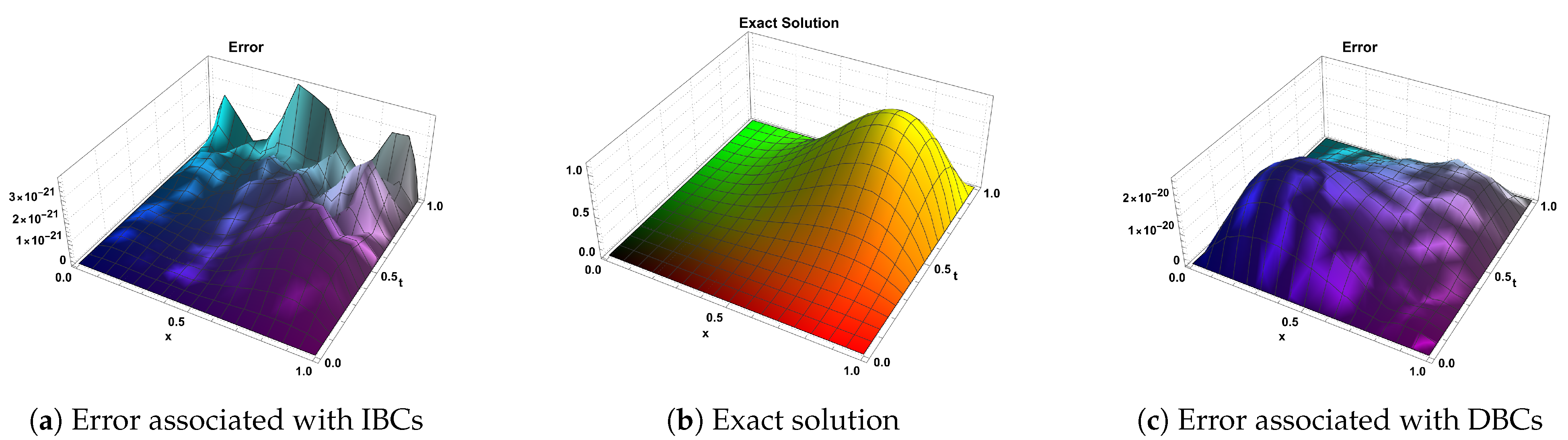
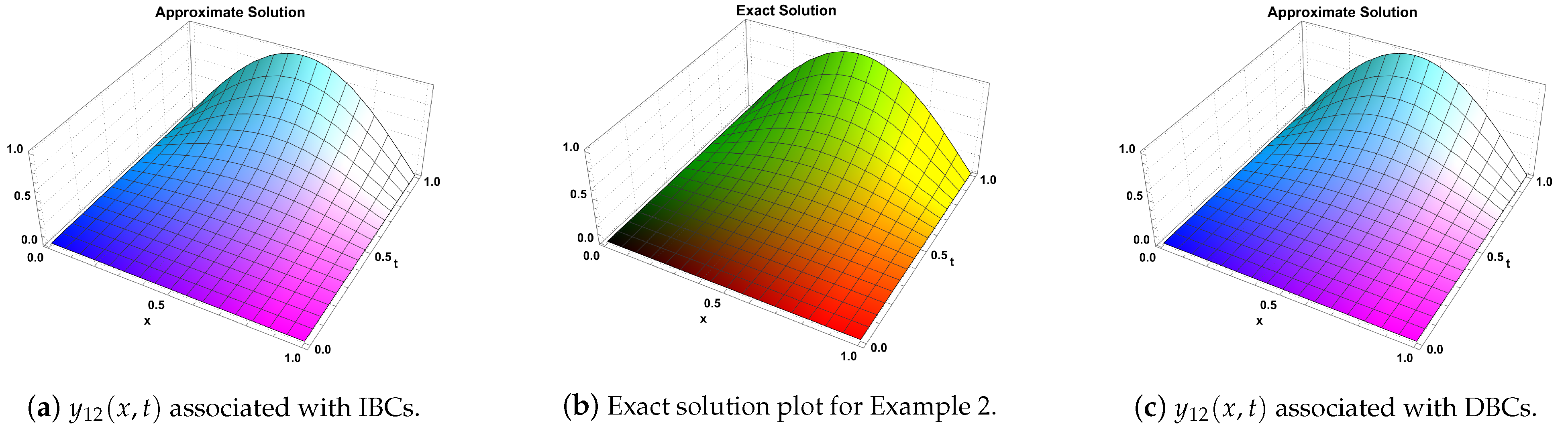
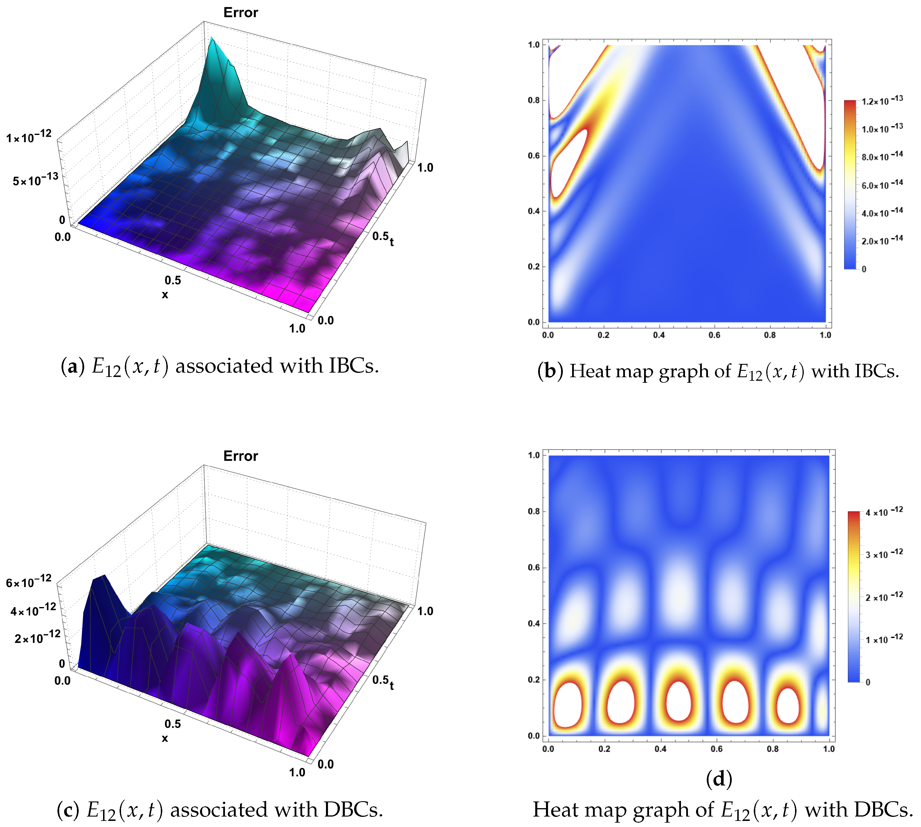
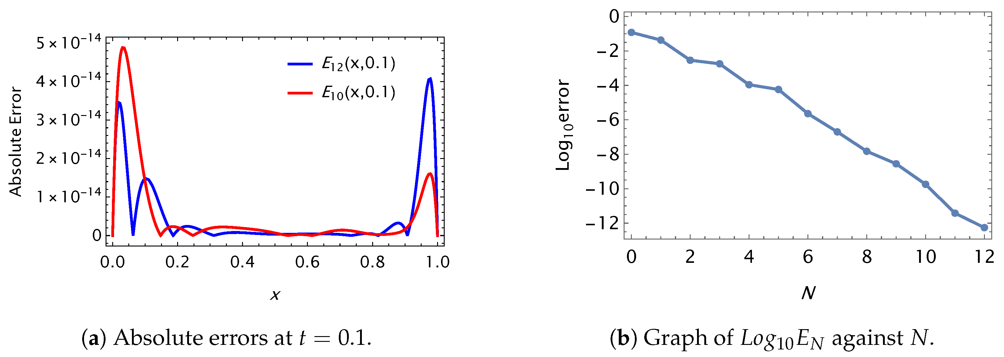
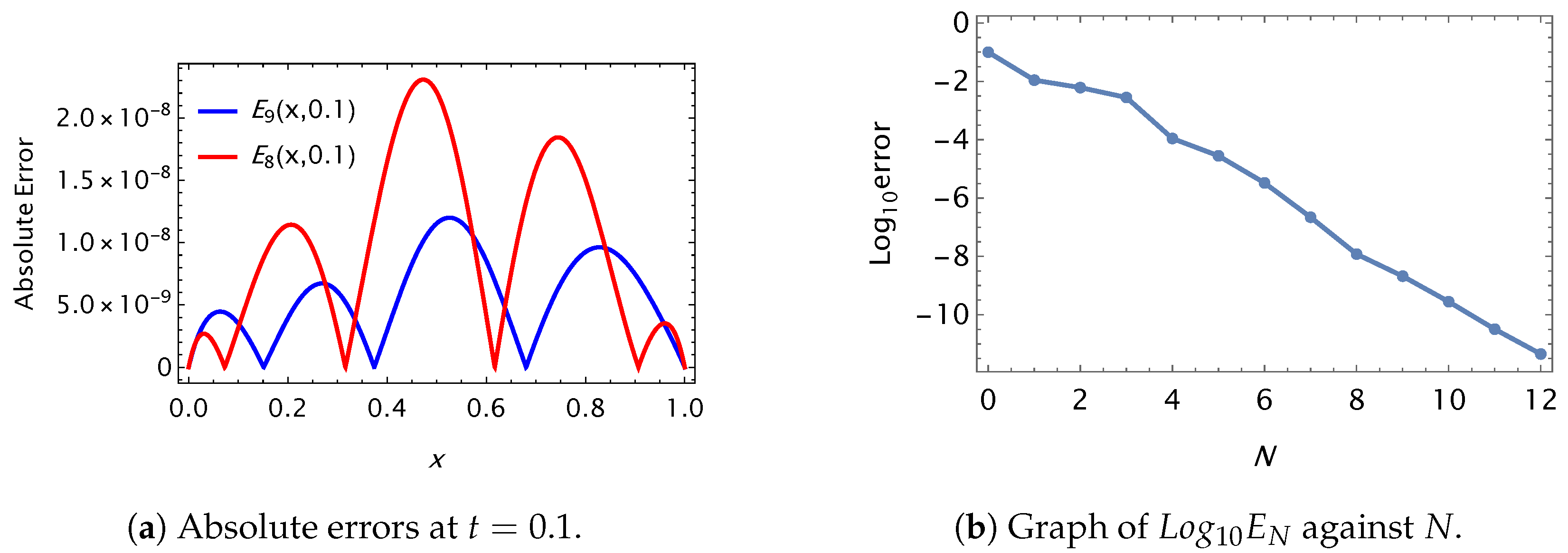
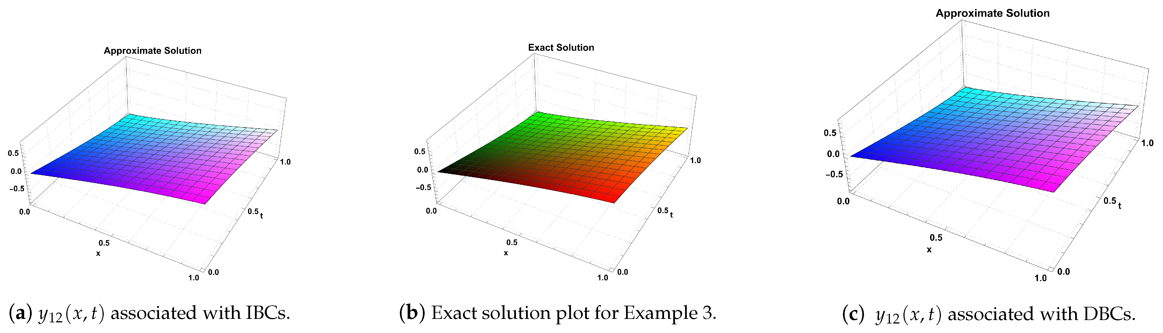
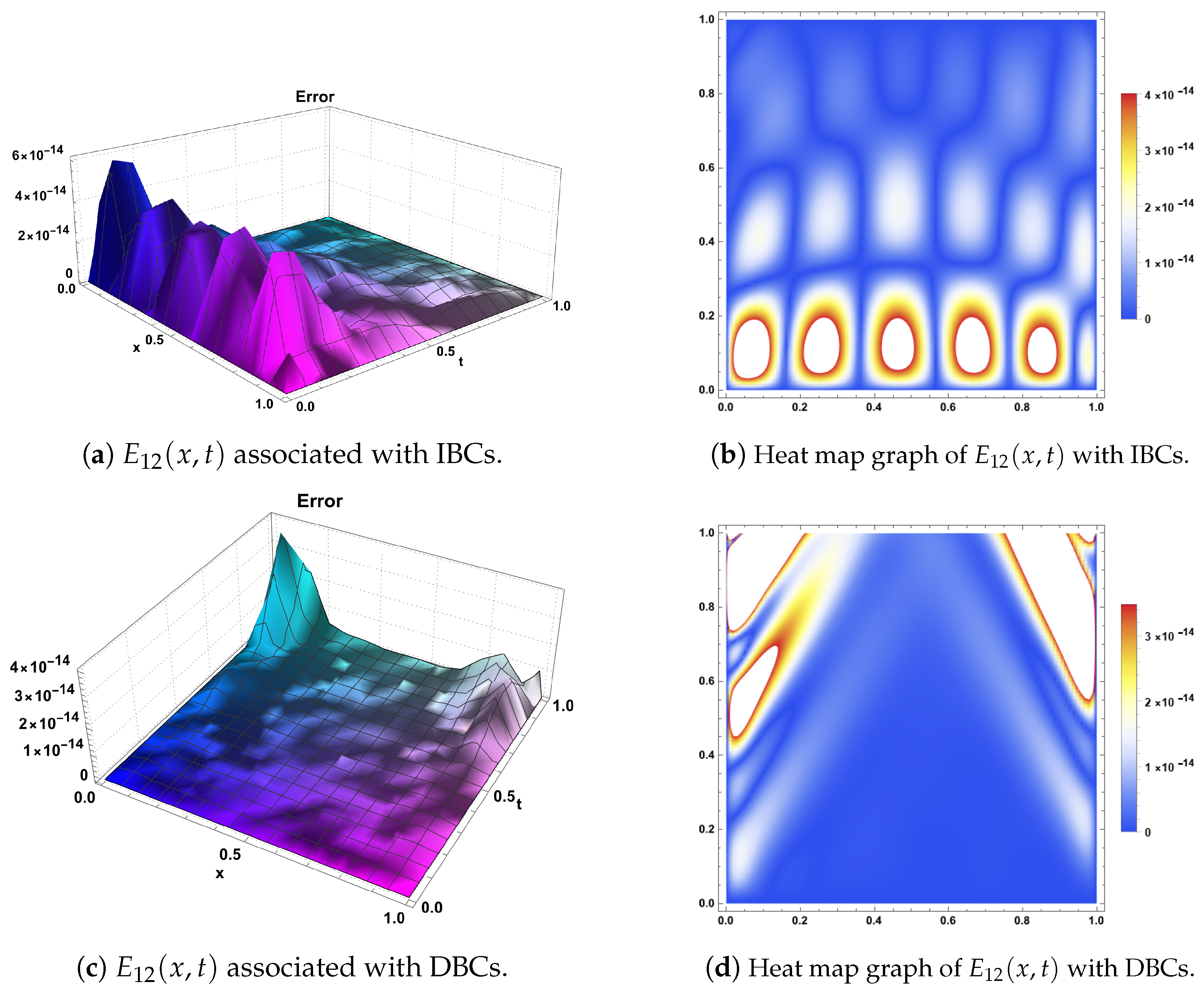
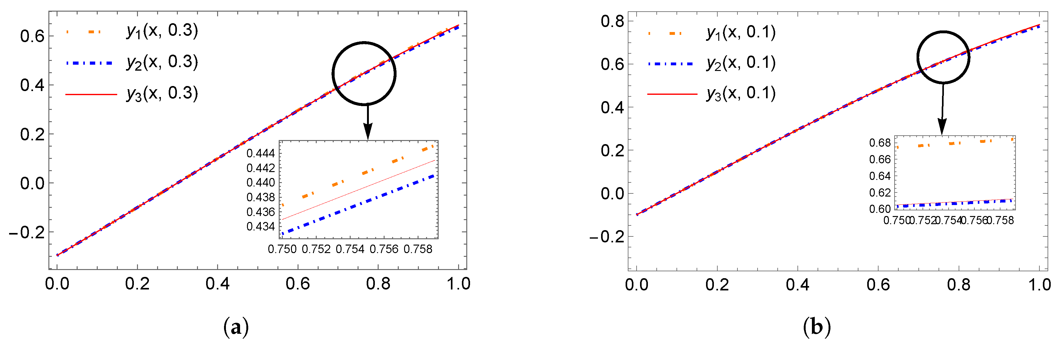
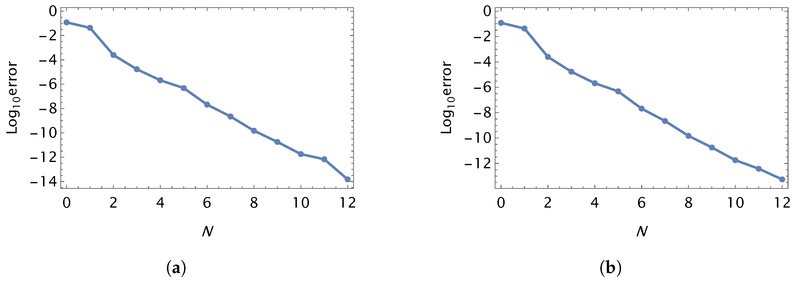
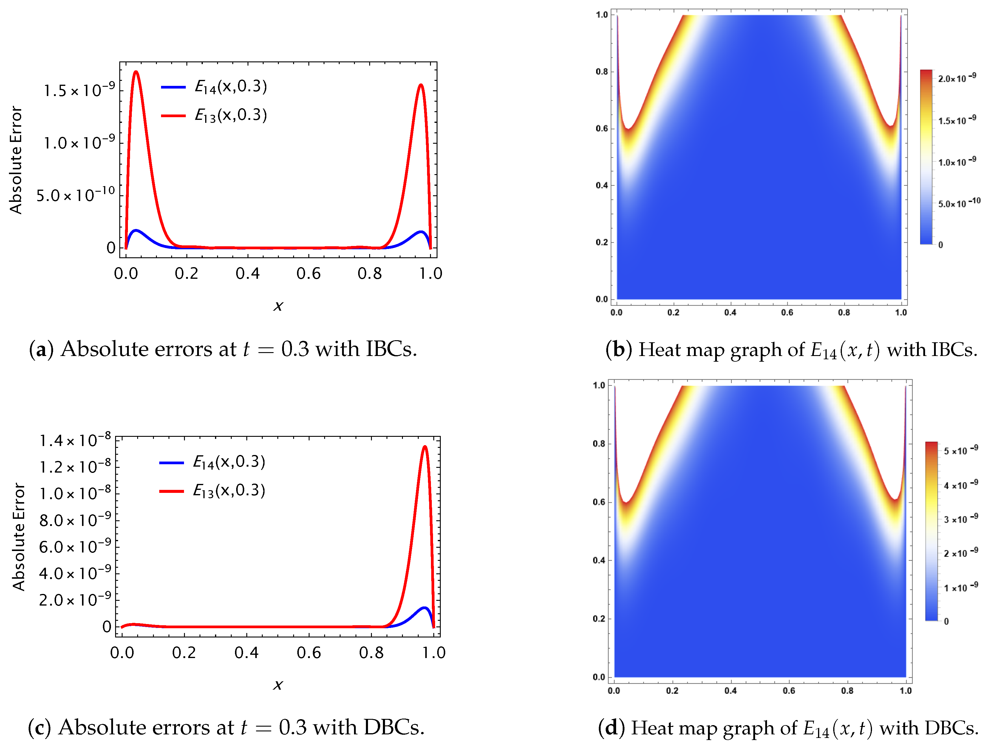
8. Numerical Simulations

In order to show how the approach presented in Section 6 works and how efficient it is, four examples are provided in this section. The assessment is based on MAE between the precise and approximate solutions. We show in Example 1 that, for certain simple cases of the functions ν ( x , t ) and ν j ( x , t ) , j = 1 , 2 , , m , we can use G S J C O P M M to find the precise solution to the given numerical problem, whether it involves IBCs or DBCs, and that it has a polynomial solution of degree N. This solution can be found by combining ψ , i ( α ^ , β ^ ) ( x ) , ϕ T , j ( α ^ , β ^ ) ( t ) , i , j = 0 , 1 , , N 2 . Otherwise, some numerical solutions are obtained with high accuracy. Additionally, the choice of examples in our study is motivated by the desire to cover different conditions, compare with existing results, showcase accuracy and efficiency, and demonstrate practical relevance. These examples collectively provide a comprehensive assessment of the performance and applicability of our proposed method for solving MTVO-TFDWEs.
In addition, Table 1, Table 2, Table 3, and Table 4 display the calculated errors that were obtained to produce numerical solutions y N ( x , t ) using G S J C O P M M with N = 0 , 1 , , 14. In these tables, excellent computational results are obtained. The comparisons between G S J C O P M M and other techniques in [57,58] are presented in Table 5 and Table 6. The tables show that, compared to the other methods, G S J C O P M M gives the most accurate results. Furthermore, as can be seen in Figure 1, Figure 2, Figure 3, Figure 4a, Figure 5a, Figure 6, Figure 7, Figure 8a, Figure 9a, and Figure 10, the precise and approximate solutions in Examples 1–4 have a high level of agreement. The absolute and log errors in Figure 4b, Figure 5b, and Figure 9 serve to illustrate the convergence and stability of the solutions to the given Problems 2 and 3 when applying G S J C O P M M and using different N , α ^ , and β ^ . The choice of parameter combinations enables us to fine-tune our method, which leads to the most accurate results.
Problem  1.
Consider the following MTVO-TFDE equation [57,58]:
D 0 c t ν ( x , t ) y ( x , t ) + D 0 c t ν 1 ( x , t ) y ( x , t ) + y t ( x , t ) = y x x ( x , t ) + g ( x , t ) , ( x , t ) [ 0 , 1 ] × [ 0 , 1 ] ,
subject to IBCs:
y ( x , 0 ) = 0 , y t ( x , 0 ) = 0 , y ( 0 , t ) = 0 , y ( 1 , t ) = 0 ,
or DBCs:
y ( x , 0 ) = 0 , y ( x , 1 ) = 0 , y ( 0 , t ) = 0 , y ( 1 , t ) = 0 ,
where g ( x , t ) is selected such that the solution to (94) is y ( x , t ) = 100 x 3 t 3 ( 1 x ) ( 1 t ) .
The application of G S J C O P M M to obtain approximated solutions with the two cases of IBCs (95) and DBCs (96) using N = 2 , , 7 , ν ( x , t ) = 2 0.3 e x t and ν 1 ( x , t ) = 2 0.6 e x t gives acceptable accuracy, as shown in Table 1. Figure 1a,c demonstrates that the obtained solutions achieve an accuracy of 10 21 at N = 7 , aligning with the exact solution depicted in Figure 1b.
Remark 4.
It is worth noting that, although the precise solution to (94) is a polynomial, the obtained approximate solutions did not give this precise solution; this is because of the complexity form of the two functions ν ( x , t ) , ν 1 ( x , t ) . However, in other special cases, for instance, ν ( x , t ) = x t , ν 1 ( x , t ) = 2 x t , for all available values of α ^ and β ^ , the precise solution is obtained using N = 2 , where the expansion coefficients c i , j = 0 , i , j = 0 , 1 , 2 , have the form:
c 0 , 0 = 100 α ^ β ^ 3 + 4 α ^ β ^ 2 + 5 α ^ β ^ + 2 α ^ + β ^ 3 + 4 β ^ 2 + 5 β ^ + 2 ( α ^ + β ^ + 2 ) 2 ( α ^ + β ^ + 3 ) 2 , c 0 , 1 = 200 α ^ β ^ 2 + 3 α ^ β ^ + 2 α ^ + β ^ 2 + 3 β ^ + 2 ( α ^ + β ^ + 2 ) 2 ( α ^ + β ^ + 3 ) ( α ^ + β ^ + 4 ) , c 0 , 2 = 200 ( α ^ β ^ + α ^ + β ^ + 1 ) ( α ^ + β ^ + 2 ) ( α ^ + β ^ + 3 ) 2 ( α ^ + β ^ + 4 ) , c 1 , 0 = 100 α ^ β ^ 2 3 α ^ β ^ 2 α ^ + β ^ 3 + 3 β ^ 2 + 2 β ^ ( α ^ + β ^ + 2 ) 2 ( α ^ + β ^ + 3 ) ( α ^ + β ^ + 4 ) , c 1 , 1 = 200 ( β ^ + 2 ) ( β ^ α ^ ) ( α ^ + β ^ + 2 ) 2 ( α ^ + β ^ + 4 ) 2 , c 1 , 2 = 200 ( β ^ α ^ ) ( α ^ + β ^ + 2 ) ( α ^ + β ^ + 3 ) ( α ^ + β ^ + 4 ) 2 , c 2 , 0 = 200 β ^ 2 + 3 β ^ + 2 ( α ^ + β ^ + 2 ) ( α ^ + β ^ + 3 ) 2 ( α ^ + β ^ + 4 ) , c 2 , 1 = 400 ( β ^ + 2 ) ( α ^ + β ^ + 2 ) ( α ^ + β ^ + 3 ) ( α ^ + β ^ + 4 ) 2 , c 2 , 2 = 400 ( α ^ + β ^ + 3 ) 2 ( α ^ + β ^ + 4 ) 2 .
Remark 5.
Although errors smaller than 10 16 may not have direct practical significance, increasing the value of N can still meaningfully improve accuracy in numerical computations. The choice of N depends on the specific requirements and desired level of accuracy for the problem under consideration. We emphasize that the relative improvement in accuracy should be considered when evaluating the meaningfulness of different values of N.
Problem  2.
Consider the following MTVO-TFDE equation [57,58]:
D 0 c t ν ( x , t ) + j = 1 4 1 j + 1 D 0 c t ν j ( x , t ) y ( x , t ) + y t ( x , t ) = 1 3 y x x ( x , t ) + g ( x , t ) , ( x , t ) [ 0 , 1 ] × [ 0 , 1 ] ,
subject to IBCs:
y ( x , 0 ) = 0 , y t ( x , 0 ) = 0 , y ( 0 , t ) = 0 , y ( 1 , t ) = 0 ,
or DBCs:
y ( x , 0 ) = 0 , y ( x , 1 ) = sin ( π x ) , y ( 0 , t ) = 0 , y ( 1 , t ) = 0 ,
where g ( x , t ) is selected such that the solution to (97) is y ( x , t ) = t 3 sin ( π x ) .
The application of G S J C O P M M to obtain approximated solutions to (97), subject to IBCs (98) or DBCs (99), respectively, using N = 0 , 1 , 2 , 5 , 8 , 12 , ν ( x , t ) = 2 0.3 e x t and ν j ( x , t ) = 2 ( 0.1 ) ( j + 3 ) e x t , j = 1 , 2 , 3 , 4 , gives acceptable accuracy, as shown in Table 2. Figure 3a,c demonstrates that the obtained solutions achieve an accuracy of 10 13 at N = 12 , aligning with the approximate and exact solutions depicted in Figure 2. Additionally, we may obtain valuable insights into the developments gained by applying G S J C O P M M from the heat map graphs displayed in Figure 3b,d and supported by the error graphs in Figure 4a and Figure 5a.
Problem  3.
Consider the following MTVO-TFDE equation [57,58]:
D 0 c t ν ( x , t ) + j = 1 5 1 j + 1 D 0 c t ν j ( x , t ) y ( x , t ) + 1 2 y t ( x , t ) = 1 3 y x x ( x , t ) + g ( x , t ) , ( x , t ) [ 0 , 1 ] × [ 0 , 1 ] ,
subject to IBCs:
y ( x , 0 ) = sin ( x ) , y t ( x , 0 ) = cos ( x ) , y ( 0 , t ) = sin ( t ) , y ( 1 , t ) = sin ( 1 t ) ,
or DBCs:
y ( x , 0 ) = sin ( x ) , y ( x , 1 ) = sin ( x 1 ) , y ( 0 , t ) = sin ( t ) , y ( 1 , t ) = sin ( 1 t ) ,
where g ( x , t ) is selected such that the solution to (100) is y ( x , t ) = sin ( x t ) .
The application of G S J C O P M M to obtain approximated solutions to (100) subject to IBCs (101) or DBCs (102), respectively, using N = 2 , 4 , 6 , 8 , 10 , 12 , ν ( x , t ) = 1.8 + 0.2 sin ( x t ) and ν j ( x , t ) = 1.8 ( 0.1 ) j + 0.2 sin ( x t ) , j = 1 , 2 , 3 , 4 , 5 , gives acceptable accuracy for the solutions obtained, as shown in Table 3 and Figure 7a,c. These solutions reach an agreement of an accuracy of 10 14 at N = 12 , aligning with the approximate and exact solutions depicted in Figure 6. Again, the heat map graphs displayed in Figure 7b,d and the error graphs in Figure 8a and Figure 9a confirm the effectiveness of G S J C O P M M .
Remark 6.
In view of the presented CPU time (in seconds), our approach has efficient performance. The calculations show that the memory consumption was excellent. For example, the calculated CPU time using N = 10 is 6% slower than N = 7 and, moreover, requires increasing by 20% the memory consumption of RAM compared to the N = 7 calculation. The numerical examples and comparisons provided in our paper highlight the superior accuracy and efficiency of our algorithm, solidifying its potential for solving MTVO-TFDEs effectively. When we compared the resource use of our method to that described in [57,58], we saw that those papers did not provide CPU time and memory usage. However, based on our analysis, our approach demonstrates better performance compared to the referenced methods.
Problem  4.
Consider the following MTVO-TFDE equation:
D 0 c t ν ( x , t ) + j = 1 2 D 0 c t ν j ( x , t ) y ( x , t ) + y t ( x , t ) = y x x ( x , t ) + g ( x , t ) , ( x , t ) [ 0 , 1 ] × [ 0 , 1 ] ,
subject to IBCs:
y ( x , 0 ) = E 1 2 , 0 ( x ) + 1 , y t ( x , 0 ) = 2 π , y ( 0 , t ) = e t 2 ( 1 + e r f ( t ) ) , y ( 1 , t ) = e t 2 ( 1 + e r f ( t ) ) + E 1 2 , 0 ( 1 ) ,
or DBCs:
y ( x , 0 ) = E 1 2 , 0 ( x ) + 1 , y ( x , 1 ) = ( 1 + e r f ( 1 ) ) e + E 1 2 , 0 ( x ) , y ( 0 , t ) = e t 2 ( 1 + e r f ( t ) ) , y ( 1 , t ) = e t 2 ( 1 + e r f ( t ) ) + E 1 2 , 0 ( 1 ) ,
where g ( x , t ) is selected such that the solution of (103) is
y ( x , t ) = E 1 2 , 1 ( t ) + E 1 2 , 0 ( x ) ,
and where the functions
e r f ( x ) = 2 π 0 x e t 2 d t and E α , β ( x ) = k = 0 x k Γ ( k α + β ) ,
are the Gaussian error function and the generalized Mitta–Leffler function, respectively. The application of G S J C O P M M to obtain approximated solutions to (103) subject to IBCs (104) or DBCs (105), respectively, using N = 2 , 4 , 6 , 8 , 10 , 14 , ν ( x , t ) = 1 + x t and ν 1 ( x , t ) = 2 x t , ν 2 ( x , t ) = 3 2 1 4 x t , gives acceptable accuracy, as shown in Table 4, and error graphs as shown in Figure 10. These solutions reach an agreement of an accuracy of 10 9 at N = 14 .

9. Conclusions

This study presents a generalized form of shifted JPs that fulfill homogeneous IBCs or DBCs. Then, by making use of the OMs derived in Section 4 and Section 5 with the SCM, an approximation algorithm for the given MTVO-TFDWE is established. Three examples, including MTVO-TFDWE (1), were tested using the suggested technique, G S J C O P M M , to prove its high accuracy and efficiency. The examples were subjected to either the IBCs (2) or the DBCs (3). It would be great to see our results generalized to other kinds of initial and boundary conditions. Studying the system’s behavior in different settings would provide interesting insights and make our conclusions even more applicable. Additionally, the theoretical results obtained in this study can be developed to deal with more complex versions of MTVO-TFDWEs, such as multi-dimensional multi-term Caputo’s time-fractional mixed sub-diffusion and diffusion-wave equations. Additionally, incorporating adaptive strategies and parallel computing techniques could further enhance the efficiency and scalability of the algorithm. Overall, this research contributes to the advancement of numerical methods for MTVO-TFDWEs and opens up avenues for exploring their applications in various fields.

Funding

This research received no external funding.

Data Availability Statement

No new data were created or analyzed in this study. Data sharing is not applicable to this article.

Acknowledgments

The author is grateful to the reviewers and editor for their insightful comments and recommendations, which substantially enhanced this research.

Conflicts of Interest

The author declare no conflict of interest.

Abbreviations

The following abbreviations are used in this manuscript:
AbbreviationDescription
DEsDifferential equations
FDEsFractional differential equations
VOFDEsVariable-order fractional differential equations
MTVOMulti-term variable-order
TFDWEsTime-fractional diffusion-wave equations
MTVO-TFDWEsMulti-term variable-order time-fractional diffusion-wave equations
IBCsInitial boundary conditions
DBCsDirichlet boundary conditions
OMsOperational matrices
OdsOrdinary derivatives
VOFDsVariable-order fractional derivatives
SCMSpectral collocation method
VOFCVariable-order fractional calculus
JPsJacobi polynomials
GSJPsGeneralized shifted Jacobi polynomials
GSJCOPMMGeneralized shifted Jacobi collocation operational matrix method
BPABest possible approximation
MAEMaximum absolute error

References

  1. Maayah, B.; Arqub, O.A.; Alnabulsi, S.; Alsulami, H. Numerical solutions and geometric attractors of a fractional model of the cancer-immune based on the Atangana–Baleanu–Caputo derivative and the reproducing kernel scheme. Chinese J. Phys. 2022, 80, 463–483. [Google Scholar] [CrossRef]
  2. Berredjem, N.; Maayah, B.; Arqub, O.A. A numerical method for solving conformable fractional integrodifferential systems of second-order, two-points periodic boundary conditions. Alex. Eng. J. 2022, 61, 5699–5711. [Google Scholar] [CrossRef]
  3. Arqub, O.A.; Rabah, A.B.; Momani, S. A spline construction scheme for numerically solving fractional Bagley–Torvik and Painlevé models correlating initial value problems concerning the Caputo–Fabrizio derivative approach. Int. J. Mod. Phys. C 2023, 34, 2350115. [Google Scholar] [CrossRef]
  4. Almeida, R.; Tavares, D.; Torres, D.F.M. The Variable-Order Fractional Calculus of Variations; Springer: Cham, Switzerland, 2019. [Google Scholar]
  5. Podlubny, I. Fractional Differential Equations; Academic Press: San Diego, CA, USA, 1999. [Google Scholar]
  6. Kilbas, A.A.; Srivastava, H.M.; Trujillo, J.J. Theory and Applications of Fractional Differential Equations; Elsevier: Amsterdam, The Netherlands, 2006; Volume 204. [Google Scholar]
  7. Mainardi, F. Fractional Calculus and Waves in Linear Viscoelasticity; Imperial College Press: London, UK, 2010. [Google Scholar]
  8. Samko, S.G.; Ross, B. Integration and differentiation to a variable fractional order. Integr. Transf. Spec. Funct. 1993, 1, 277–300. [Google Scholar] [CrossRef]
  9. Odzijewicz, T.; Malinowska, A.B.; Torres, D.F.M. Noether’s theorem for fractional variational problems of variable order. Cent. Eur. J. Phys. 2013, 11, 691–701. [Google Scholar] [CrossRef]
  10. Chen, S.; Liu, F.; Burrage, K. Numerical simulation of a new two-dimensional variable-order fractional percolation equation in non-homogeneous porous media. Comput. Math. Appl. 2014, 67, 1673–1681. [Google Scholar] [CrossRef]
  11. Coimbra, C.F.M.; Soon, C.M.; Kobayashi, M.H. The variable viscoelasticity operator. Ann. Phys. 2005, 14, 378–389. [Google Scholar]
  12. Odzijewicz, T.; Malinowska, A.B.; Torres, D.F.M. Fractional variational calculus of variable order. In Advances in Harmonic Analysis and Operator Theory: Advances and Applications; Almeida, A., Castro, L., Speck, F.O., Eds.; Birkhäuser: Basel, Switzerland, 2013; Volume 229, pp. 291–301. [Google Scholar]
  13. Ostalczyk, P.W.; Duch, P.; Brzeziński, D.W.; Sankowski, D. Order functions selection in the variable-fractional-order PID controller. Advances in Modelling and Control of Non-integer-Order Systems. Lect. Notes Electr. Eng. 2015, 320, 159–170. [Google Scholar]
  14. Rapaić, M.R.; Pisano, A. Variable-order fractional operators for adaptive order and parameter estimation. IEEE Trans. Autom. Contr. 2013, 59, 798–803. [Google Scholar] [CrossRef]
  15. Izadi, M.; Yüzbasi, S.; Adel, W. Two novel Bessel matrix techniques to solve the squeezing flow problem between infinite parallel plates. Comput. Math. Math. Phy. 2021, 61, 2034–2053. [Google Scholar] [CrossRef]
  16. Coimbra, C.F.M. Mechanics with variable-order differential operators. AdP 2003, 515, 692–703. [Google Scholar] [CrossRef]
  17. Lin, R.; Liu, F.; Anh, V.; Turner, I. Stability and convergence of a new explicit finite-difference approximation for the variable-order nonlinear fractional diffusion equation. Appl. Math. Comput. 2009, 212, 435–445. [Google Scholar] [CrossRef]
  18. Birajdar, G.A.; Rashidi, M.M. Finite Difference Schemes for Variable Order Time-Fractional First Initial Boundary Value Problems. Appl. Appl. Math. 2017, 12, 112–135. [Google Scholar]
  19. Patnaik, S.; Semperlotti, F. Variable-order particle dynamics: Formulation and application to the simulation of edge dislocations. Philos. Trans. R. Soc. A 2020, 378, 0190290. [Google Scholar] [CrossRef] [PubMed]
  20. Blaszczyk, T.; Bekus, K.; Szajek, K.; Sumelka, W. Approximation and application of the Riesz-caputo fractional derivative of variable order with fixed memory. Meccanica 2022, 57, 861–870. [Google Scholar] [CrossRef]
  21. Abd-Elhameed, W.M.; Ahmed, H.M. Spectral solutions for the time-fractional heat differential equation through a novel unified sequence of Chebyshev polynomials. AIMS Math. 2024, 9, 2137–2166. [Google Scholar] [CrossRef]
  22. Paola, M.D.; Alotta, G.; Burlon, A.; Failla, G. A novel approach to nonlinear variable-order fractional viscoelasticity. Philos. Trans. R. Soc. A 2020, 378, 20190296. [Google Scholar] [CrossRef] [PubMed]
  23. Burlon, A.; Alotta, G.; Paola, M.D.; Failla, G. An original perspective on variable-order fractional operators for viscoelastic materials. Meccanica 2021, 56, 769–784. [Google Scholar] [CrossRef]
  24. Ahmed, H.M. A new first finite class of classical orthogonal polynomials operational matrices: An application for solving fractional differential equations. Contemp. Math. 2023, 4, 974–994. [Google Scholar] [CrossRef]
  25. Napoli, A.; Abd-Elhameed, W.M. An innovative harmonic numbers operational matrix method for solving initial value problems. Calcolo 2017, 54, 57–76. [Google Scholar] [CrossRef]
  26. Izadi, M.; Yüzbasi, S.; Adel, W. A new Chelyshkov matrix method to solve linear and nonlinear fractional delay differential equations with error analysis. Math. Sci. 2023, 17, 267–284. [Google Scholar] [CrossRef]
  27. Izadi, M.; Sene, N.; Adel, W.; El-Mesady, A. The Layla and Majnun mathematical model of fractional order: Stability analysis and numerical study. Results Phys. 2023, 51, 106650. [Google Scholar] [CrossRef]
  28. Liu, J.; Li, X.; Wu, L. An operational matrix of fractional differentiation of the second kind of Chebyshev polynomial for solving multiterm variable order fractional differential equation. Math. Probl. Eng. 2016, 2016, 7126080. [Google Scholar] [CrossRef]
  29. Youssri, Y.H.; Abd-Elhameed, W.M.; Ahmed, H.M. New fractional derivative expression of the shifted third-kind Chebyshev polynomials: Application to a type of nonlinear fractional pantograph differential equations. J. Funct. Spaces 2022, 2022, 3966135. [Google Scholar] [CrossRef]
  30. Abd-Elhameed, W.M.; Alkenedri, A.M. New formulas for the repeated integrals of some Jacobi polynomials: Spectral solutions of even-order boundary value problems. Int. J. Appl. Comput. Math. 2021, 7, 166. [Google Scholar] [CrossRef]
  31. Sheikhi, S.; Matinfar, M.; Firoozjaee, M.A. Numerical solution of variable-order differential equations via the Ritz-approximation method by shifted Legendre polynomials. Int. J. Appl. Comput. Math. 2021, 7, 22. [Google Scholar] [CrossRef]
  32. El-Sayed, A.A.; Baleanu, D.; Agarwal, P. A novel Jacobi operational matrix for numerical solution of multi-term variable-order fractional differential equations. J. Taibah Univ. Sci. 2020, 14, 963–974. [Google Scholar] [CrossRef]
  33. Nagy, A.M.; Sweilam, N.H.; El-Sayed, A.A. New operational matrix for solving multiterm variable order fractional differential equations. J. Comp. Nonlinear Dyn. 2018, 13, 011001–011007. [Google Scholar] [CrossRef]
  34. El-Sayed, A.A.; Agarwal, P. Numerical solution of multiterm variable-order fractional differential equations via shifted Legendre polynomials. Math. Meth. Appl. Sci. 2019, 42, 3978–3991. [Google Scholar] [CrossRef]
  35. Wang, L.F.; Ma, Y.P.; Yang, Y.Q. Legendre polynomials method for solving a class of variable order fractional differential equation. CMES-Comp. Model. Eng. 2014, 101, 97–111. [Google Scholar]
  36. Chen, Y.M.; Wei, Y.Q.; Liu, D.Y.; Yu, H. Numerical solution for a class of nonlinear variable order fractional differential equations with Legendre wavelets. Appl. Math. Lett. 2015, 46, 83–88. [Google Scholar] [CrossRef]
  37. Bushnaq, S.; Shah, K.; Tahir, S.; Ansari, K.J.; Sarwar, M.; Abdeljawad, T. Computation of numerical solutions to variable order fractional differential equations by using non-orthogonal basis. AIMS Math. 2022, 7, 10917–10938. [Google Scholar] [CrossRef]
  38. Chen, Y.M.; Liu, L.Q.; Li, B.F.; Sun, Y. Numerical solution for the variable order linear cable equation with Bernstein polynomials. Appl. Math. Comput. 2014, 238, 329–341. [Google Scholar] [CrossRef]
  39. Shen, S.; Liu, F.; Chen, J.; Turner, I.; Anh, V. Numerical techniques for the variable order time fractional diffusion equation. Appl. Math. and Comput. 2012, 218, 10861–10870. [Google Scholar] [CrossRef]
  40. Moghaddam, B.P.; Machado, J.A.T. Extended algorithms for approximating variable order fractional derivatives with applications. J. Sci. Comput. 2017, 71, 1351–1374. [Google Scholar] [CrossRef]
  41. Ahmed, H.M. Enhanced shifted Jacobi operational matrices of derivatives: Spectral algorithm for solving multiterm variable-order fractional differential equations. Bound. Value Probl. 2023, 2023, 108. [Google Scholar] [CrossRef]
  42. Shen, J.; Tang, T.; Wang, L. Spectral Methods: Algorithms, Analysis and Applications; Springer: Berlin/Heidelberg, Germany, 2011; Volume 41. [Google Scholar]
  43. Abd-Elhameed, W.M.; Ahmed, H.M.; Youssri, Y.H. A new generalized Jacobi Galerkin operational matrix of derivatives: Two algorithms for solving fourth-order boundary value problems. Adv. Differ. Equ. 2016, 2016, 22. [Google Scholar] [CrossRef]
  44. Abd-Elhameed, W.M.; Ahmed, H.M. Tau and Galerkin operational matrices of derivatives for treating singular and Emden-Fowler third-order-type equations. Int. J. Mod. Phys. C 2022, 33, 2250061. [Google Scholar] [CrossRef]
  45. Heydari, M.H.; Hooshmandasl, M.R.; Ghaini, F.M.M.; Cattani, C. Wavelets method for the time fractional diffusion-wave equation. Phys. Lett. A 2015, 379, 71–76. [Google Scholar] [CrossRef]
  46. Jiang, H.; Liu, F.; Turner, I.; Burrage, K. Analytical solutions for the multi-term time-fractional diffusion-wave/diffusion equations in a finite domain. Comput. Math. Appl. 2012, 64, 3377–3388. [Google Scholar] [CrossRef]
  47. Nigmatullin, R.R. To the theoretical explanation of the universal response. Phys. Status Solidi (B) Basic Res. 1984, 123, 739–745. [Google Scholar] [CrossRef]
  48. Nigmatullin, R.R. Realization of the generalized transfer equation in a medium with fractal geometry, phys. status solidi, b basic res. Phys. Status Solidi (B) Basic Res. 1986, 133, 425–430. [Google Scholar] [CrossRef]
  49. Luchko, Y. Initial-boundary-value problems for the generalized multi-term time-fractional diffusion equation. J. Math. Anal. Appl. 2011, 374, 538–548. [Google Scholar] [CrossRef]
  50. Liu, Y.; Yamamoto, M. Uniqueness of orders and parameters in multi-term time-fractional diffusion equations by short-time behavior. Inverse Probl. 2022, 39, 024003. [Google Scholar] [CrossRef]
  51. Cheng, J.; Nakagawa, J.; Yamamoto, M.; Yamazaki, T. Uniqueness in an inverse problem for a one dimensional fractional diffusion equation. Inverse Probl. 2009, 25, 115002. [Google Scholar] [CrossRef]
  52. Szegö, G. Orthogonal Polynomials, 4th ed.; American Mathematical Soc.: Providence, RI, USA, 1975; Volume XXIII. [Google Scholar]
  53. Luke, Y.L. Mathematical Functions and Their Approximations; Academic Press: London, UK, 1975. [Google Scholar]
  54. Prudnikov, A.P.; Brychkov, Y.A.; Marichev, O.I. More Special Functions; Integrals and Series; Gordon and Breach: New York, NY, USA, 1990; Volume 3. [Google Scholar]
  55. Narumi, S. Some formulas in the theory of interpolation of many independent variables. Tohoku Math. J. 1920, 18, 309–321. [Google Scholar]
  56. Jeffrey, A.; Dai, H.H. Handbook of Mathematical Formulas and Integrals, 4th ed.; Elsevier: Amsterdam, The Netherlands, 2008. [Google Scholar]
  57. Heydari, M.H.; Avazzadeh, Z.; Haromi, M.F. A wavelet approach for solving multi-term variable-order time fractional diffusion-wave equation. Appl. Math. Comput. 2019, 341, 215–228. [Google Scholar] [CrossRef]
  58. Sadri, K.; Aminikhah, H. A new efficient algorithm based on fifth-kind Chebyshev polynomials for solving multi-term variable-order time-fractional diffusion-wave equation. Int. J. Comput. Math. 2022, 99, 966–992. [Google Scholar] [CrossRef]
Figure 1. Exact solution and error plots for Example 1 using α ^ = 0 , β ^ = 1 / 2 and N = 7 .
Fractalfract 08 00068 g001
Figure 2. Exact and approximate solutions using ( N = 12 , α ^ = 0 , β ^ = 1 / 2 ) for Example 2.
Fractalfract 08 00068 g002
Figure 3. Error functions and their heat map graphs using ( N = 12 , α ^ = 0 , β ^ = 1 / 2 ) for Example 2.
Fractalfract 08 00068 g003
Figure 4. Error results using ( α ^ = 0 , β ^ = 1 / 2 ) for Example 2 associated with IBCs.
Fractalfract 08 00068 g004
Figure 5. Error results using ( α ^ = 0 , β ^ = 1 / 2 ) for Example 2 associated with DBCs.
Fractalfract 08 00068 g005
Figure 6. Exact and approximate solutions using ( N = 12 , α ^ = β ^ = 1 / 2 ) for Example 3.
Fractalfract 08 00068 g006
Figure 7. Error functions and their heat map graphs using ( N = 12 , α ^ = β ^ = 1 / 2 ) for Example 3.
Fractalfract 08 00068 g007
Figure 8. Approximate solution plots for Example 3 associated with IBCs or DBCs using ( N = 1 , 2 , 3 , α ^ = β ^ = 1 / 2 ) . (a) Approximate solution plots at t = 0.3 associated with IBCs; (b) approximate solution plots t = 0.1 associated with DBCs.
Fractalfract 08 00068 g008
Figure 9. Graph of L o g 10 E N for Example 3 associated with IBCs (a) or DBCs (b) using ( N = 0 , 1 , , 12 , α ^ = β ^ = 1 / 2 ) .
Fractalfract 08 00068 g009
Figure 10. Error results and their heat map graphs using ( α ^ = β ^ = 1 / 2 ) for Example 4.
Fractalfract 08 00068 g010
Table 1. MAEs of Example 1 using various α ^ , β ^ , and N.
α ^ β ^ IBCs/DBCs N = 2 N = 3 N = 4 N = 5 N = 6 N = 7
00IBCs1.3 ×  10 16 2.3 ×  10 17 1.9 ×  10 18 2.4 ×  10 19 2.7 ×  10 20 2.4 ×  10 21
DBCs2.6 ×  10 16 3.4 ×  10 17 3.5 ×  10 18 3.9 ×  10 19 3.6 ×  10 20 1.6 ×  10 20
CPU time0.2310.3120.4010.4210.4510.515
1/21/2IBCs2.4 ×  10 16 1.3 ×  10 17 4.1 ×  10 18 7.2 ×  10 19 1.8 ×  10 20 2.5 ×  10 21
DBCs2.7 ×  10 16 3.6 ×  10 17 3.8 ×  10 18 3.9 ×  10 19 4.4 ×  10 20 2.7 ×  10 20
CPU time0.2320.3130.4030.4220.4530.517
−1/2−1/2IBCs1.5 ×  10 16 2.8 ×  10 17 4.8 ×  10 18 1.2 ×  10 19 1.8 ×  10 20 2.6 ×  10 21
DBCs1.6 ×  10 16 3.6 ×  10 17 1.9 ×  10 18 1.9 ×  10 19 5.4 ×  10 20 2.1 ×  10 20
CPU time0.2210.3100.4020.4220.4500.517
10IBCs3.3 ×  10 15 4.3 ×  10 16 3.7 ×  10 17 2.2 ×  10 18 1.8 ×  10 19 3.1 ×  10 21
DBCs3.9 ×  10 16 3.6 ×  10 17 2.1 ×  10 18 1.9 ×  10 19 2.6 ×  10 20 2.2 ×  10 20
CPU time0.2330.3140.4070.4250.4580.519
01IBCs4.3 ×  10 15 2.3 ×  10 16 4.5 ×  10 17 4.4 ×  10 18 1.7 ×  10 19 2.9 ×  10 21
DBCs2.9 ×  10 16 3.2 ×  10 17 2.5 ×  10 18 3.8 ×  10 19 8.6 ×  10 20 2.3 ×  10 20
CPU time0.2340.3150.4070.4260.4510.519
Table 2. MAEs of Example 2 using various α ^ , β ^ , and N.
α ^ β ^ IBCs/DBCs N = 0 N = 1 N = 2 N = 5 N = 8 N = 12
00IBCs1.2 ×  10 1 4.3 ×  10 2 2.9 ×  10 3 5.8 ×  10 5 1.5 ×  10 8 5.5 ×  10 13
DBCs1.0 ×  10 1 1.1 ×  10 2 6.1 ×  10 3 4.0 ×  10 5 1.2 ×  10 8 4.5 ×  10 12
CPU time0.1010.1220.2320.4320.5210.735
1/21/2IBCs1.3 ×  10 1 4.4 ×  10 2 2.8 ×  10 3 5.4 ×  10 5 1.2 ×  10 8 5.4 ×  10 13
DBCs1.1 ×  10 1 1.1 ×  10 2 5.9 ×  10 3 4.2 ×  10 5 1.4 ×  10 8 4.0 ×  10 12
CPU time0.1020.1230.2340.4330.5250.745
−1/2−1/2IBCs1.4 ×  10 1 3.3 ×  10 2 2.1 ×  10 3 4.9 ×  10 5 1.3 ×  10 8 5.7 ×  10 13
DBCs1.2 ×  10 1 1.3 ×  10 2 5.2 ×  10 3 3.9 ×  10 5 1.5 ×  10 8 4.7 ×  10 12
CPU time0.1010.1210.2310.4330.5200.732
10IBCs1.5 ×  10 1 3.9 ×  10 2 3.0 ×  10 3 6.0 ×  10 5 2.5 ×  10 8 4.5 ×  10 13
DBCs1.3 ×  10 1 1.4 ×  10 2 6.2 ×  10 3 3.3 ×  10 5 2.0 ×  10 8 3.5 ×  10 12
CPU time0.1040.1240.2340.4350.5210.738
01IBCs1.7 ×  10 1 4.5 ×  10 2 2.7 ×  10 3 5.1 ×  10 5 1.3 ×  10 8 5.5 ×  10 13
DBCs1.7 ×  10 1 1.6 ×  10 2 6.5 ×  10 3 4.5 ×  10 5 1.8 ×  10 8 4.1 ×  10 12
CPU time0.1020.1250.2370.4380.5290.741
Table 3. MAEs of Example 3 using various α ^ , β ^ , and N.
α ^ β ^ IBCs/DBCs N = 2 N = 4 N = 6 N = 8 N = 10 N = 12
00IBCs1.4 ×  10 4 3.3 ×  10 6 2.2 ×  10 8 4.8 ×  10 10 2.5 ×  10 12 4.4 ×  10 13
DBCs1.2 ×  10 4 2.1 ×  10 6 1.1 ×  10 8 3.2 ×  10 10 2.3 ×  10 12 6.8 ×  10 14
CPU time0.2310.4010.4510.5210.6010.735
1/21/2IBCs1.0 ×  10 4 2.1 ×  10 6 2.4 ×  10 8 4.4 ×  10 10 2.2 ×  10 12 5.4 ×  10 14
DBCs1.3 ×  10 4 2.1 ×  10 6 4.9 ×  10 8 4.3 ×  10 10 2.1 ×  10 12 4.2 ×  10 14
CPU time0.2330.4050.4540.5250.6070.740
−1/2−1/2IBCs1.5 ×  10 4 2.4 ×  10 6 2.3 ×  10 8 2.4 ×  10 10 1.4 ×  10 12 5.7 ×  10 14
DBCs1.1 ×  10 4 1.5 ×  10 6 4.2 ×  10 8 2.9 ×  10 10 3.5 ×  10 12 2.2 ×  10 13
CPU time0.2400.4100.4590.5280.6100.740
10IBCs1.2 ×  10 4 2.3 ×  10 6 3.1 ×  10 8 5.0 ×  10 10 3.5 ×  10 12 8.2 ×  10 14
DBCs1.3 ×  10 4 2.5 ×  10 6 5.2 ×  10 8 4.3 ×  10 10 3.0 ×  10 12 6.5 ×  10 14
CPU time0.2380.4090.4580.5290.6080.739
01IBCs1.8 ×  10 4 2.3 ×  10 6 2.4 ×  10 8 5.2 ×  10 10 2.3 ×  10 12 4.5 ×  10 13
DBCs1.7 ×  10 4 2.5 ×  10 6 5.5 ×  10 8 3.5 ×  10 10 2.8 ×  10 12 6.1 ×  10 14
CPU time0.2370.4070.4560.5270.6080.738
Table 4. MAEs of Example 4 using various α ^ , β ^ , and N.
α ^ β ^ IBCs/DBCs N = 2 N = 4 N = 6 N = 8 N = 10 N = 14
11IBCs1.2 ×  10 2 2.3 ×  10 3 2.0 ×  10 4 3.8 ×  10 5 2.1 ×  10 6 4.5 ×  10 9
DBCs1.1 ×  10 2 3.3 ×  10 3 2.2 ×  10 4 4.8 ×  10 5 3.1 ×  10 6 2.2 ×  10 8
CPU time0.2350.4020.4540.5220.6040.988
3/21/2IBCs1.3 ×  10 2 4.3 ×  10 3 5.0 ×  10 4 3.7 ×  10 5 2.6 ×  10 6 4.4 ×  10 9
DBCs2.2 ×  10 2 3.1 ×  10 3 2.4 ×  10 4 3.5 ×  10 5 2.7 ×  10 6 4.4 ×  10 8
CPU time0.2300.3170.4110.4300.4600.980
1/23/2IBCs2.2 ×  10 2 4.3 ×  10 3 3.0 ×  10 4 3.9 ×  10 5 2.3 ×  10 6 4.6 ×  10 9
DBCs4.2 ×  10 2 3.2 ×  10 3 1.5 ×  10 4 5.8 ×  10 5 2.9 ×  10 6 4.4 ×  10 8
CPU time0.2340.3190.4120.4290.4590.991
23IBCs3.2 ×  10 2 4.3 ×  10 3 1.0 ×  10 4 1.8 ×  10 5 2.2 ×  10 6 4.6 ×  10 9
DBCs5.2 ×  10 2 3.4 ×  10 3 2.3 ×  10 4 3.6 ×  10 5 2.0 ×  10 6 6.1 ×  10 9
CPU time0.2390.3200.4130.4300.4611.001
32IBCs1.7 ×  10 2 2.8 ×  10 3 2.5 ×  10 4 2.8 ×  10 5 2.4 ×  10 6 4.7 ×  10 9
DBCs2.3 ×  10 2 4.3 ×  10 3 2.5 ×  10 4 3.9 ×  10 5 2.8 ×  10 6 4.6 ×  10 9
CPU time0.2380.3190.4120.4280.4580.998
Table 5. The method’s comparisons [57,58] and G S J C O P M M in Example 2 with IBCs and DBCs.
GSJCOPMM (IBCs) GSJCOPMM (DBCs)[57] (IBCs)[58] (DBCs)
( x , t ) ( α ^ = β ^ = 1 , N = 10 ) ( α ^ = β ^ = 1 , N = 8 ) ( k = 1 , M = 10 ) ( N = M = 8 )
(0.1, 0.1)1.47 ×  10 14 3.15 ×  10 9 3.05 ×  10 4 1.69 ×  10 7
(0.2, 0.2)4.34 ×  10 15 1.09 ×  10 8 8.35 ×  10 6 1.12 ×  10 7
(0.3, 0.3)2.55 ×  10 15 4.39 ×  10 9 2.35 ×  10 7 1.97 ×  10 8
(0.4, 0.4)5.41 ×  10 16 1.48 ×  10 8 5.40 ×  10 7 1.33 ×  10 7
(0.5, 0.5)2.08 ×  10 16 8.08 ×  10 9 6.60 ×  10 8 1.38 ×  10 8
(0.6, 0.6)4.88 ×  10 15 3.43 ×  10 9 1.53 ×  10 7 1.36 ×  10 7
(0.7, 0.7)4.78 ×  10 13 2.28 ×  10 9 3.73 ×  10 8 1.04 ×  10 7
(0.8, 0.8)8.71 ×  10 12 1.70 ×  10 9 1.06 ×  10 7 1.90 ×  10 6
(0.9, 0.9)5.22 ×  10 11 3.71 ×  10 9 6.65 ×  10 8 4.68 ×  10 5
Table 6. The method’s comparisons [57,58] and G S J C O P M M in Example 3 with DBCs.
GSJCOPMM GSJCOPMM [58][57][57]
( x , t ) ( α ^ = β ^ = 1 , N = 10 ) ( α ^ = β ^ = 1 , N = 7 ) ( M = N = 7 ) ( k = 1 , M = 7 ) ( k = 1 , M = 10 )
(0.1, 0.1)1.39 ×  10 14 1.1 ×  10 13 1.29 ×  10 13 5.62 ×  10 8 1.04 ×  10 12
(0.2, 0.2)3.66 ×  10 15 6.2 ×  10 13 3.41 ×  10 12 1.87 ×  10 8 8.61 ×  10 12
(0.3, 0.3)2.07 ×  10 15 7.5 ×  10 13 2.37 ×  10 12 1.34 ×  10 7 1.11 ×  10 12
(0.4, 0.4)1.60 ×  10 15 1.6 ×  10 12 4.27 ×  10 11 3.25 ×  10 7 6.39 ×  10 13
(0.5, 0.5)2.58 ×  10 15 2.6 ×  10 12 9.46 ×  10 11 2.57 ×  10 7 2.06 ×  10 12
(0.6, 0.6)4.64 ×  10 15 3.3 ×  10 12 1.14 ×  10 10 1.66 ×  10 7 5.52 ×  10 12
(0.7, 0.7)2.07 ×  10 14 4.6 ×  10 12 3.26 ×  10 11 8.95 ×  10 8 3.11 ×  10 12
(0.8, 0.8)2.39 ×  10 14 1.7 ×  10 10 1.93 ×  10 9 3.78 ×  10 8 8.14 ×  10 13
(0.9, 0.9)3.60 ×  10 13 1.2 ×  10 9 1.32 ×  10 8 3.34 ×  10 8 1.89 ×  10 12
Disclaimer/Publisher’s Note: The statements, opinions and data contained in all publications are solely those of the individual author(s) and contributor(s) and not of MDPI and/or the editor(s). MDPI and/or the editor(s) disclaim responsibility for any injury to people or property resulting from any ideas, methods, instructions or products referred to in the content.

