Article

Numerical Simulation of a Space-Fractional Molecular Beam Epitaxy Model without Slope Selection

Department of Mathematics, Kwangwoon University, Seoul 01897, Republic of Korea
Fractal Fract. 2023, 7(7), 558; https://doi.org/10.3390/fractalfract7070558
Submission received: 12 May 2023 / Revised: 4 July 2023 / Accepted: 13 July 2023 / Published: 18 July 2023
(This article belongs to the Special Issue Recent Advances in Time/Space-Fractional Evolution Equations)

Abstract

:
In this paper, we introduce a space-fractional version of the molecular beam epitaxy (MBE) model without slope selection to describe super-diffusion in the model. Compared to the classical MBE equation, the spatial discretization is an important issue in the space-fractional MBE equation because of the nonlocal nature of the fractional operator. To approximate the fractional operator, we employ the Fourier spectral method, which gives a full diagonal representation of the fractional operator and achieves spectral convergence regardless of the fractional power. And, to combine with the Fourier spectral method directly, we present a linear, energy stable, and second-order method. Then, it is possible to simulate the dynamics of the space-fractional MBE equation efficiently and accurately. By using the numerical method, we investigate the effect of the fractional power in the space-fractional MBE equation.

1. Introduction

The molecular beam epitaxy (MBE) is a versatile technique for growing thin epitaxial structures made of semiconductors, metals or insulators [1]. One of models for simulating the MBE growth is the gradient flow for the following energy functional [2]:
E ( ϕ ) : = Ω 1 2 ln ( 1 + | ϕ | 2 ) + δ 2 | Δ ϕ | 2 d x ,
where ϕ is a scaled height function of a thin film in a co-moving frame and δ > 0 is a constant. The first and second terms in E ( ϕ ) model the Ehrlich–Schwoebel effect [3,4,5] and surface diffusion, respectively. Because of the first term in E ( ϕ ) , this model is characterized by the absence of a preferred slope, i.e., there is no slope selection [6]. The L 2 -gradient flow for E ( ϕ ) takes the form [6]
ϕ t = δ E δ ϕ = · ϕ 1 + | ϕ | 2 + δ Δ 2 ϕ ,
where δ δ ϕ denotes the variational derivative and the boundary condition for ϕ is considered periodic in all spatial directions. It has been shown analytically and numerically that the MBE Equation (2) predicts E ( t ) O ( ln ( t ) ) and w ( t ) O ( t 1 / 2 ) as t [6,7,8,9,10,11,12,13,14,15], where w ( t ) is the roughness (the standard deviation of the height profile) defined as [7,16]
w ( t ) = 1 | Ω | Ω ϕ ( x , t ) ϕ ¯ ( t ) 2 d x ,
where ϕ ¯ ( t ) = 1 | Ω | Ω ϕ ( x , t ) d x . One might wonder whether anomalous MBE affects the scaling rates. A straightforward idea is to utilize fractional derivatives, i.e., formulate fractional MBE equations. Fractional partial differential equations have been proved to be valuable tools for modeling diffusive processes associated with anomalous diffusion [17,18,19,20,21,22,23,24,25,26,27,28,29,30,31]. In recent years, the time-fractional version of the MBE equation has been introduced and solved numerically to describe sub-diffusion in the MBE Equation [32,33,34,35,36,37]. However, to the best of our knowledge, there is no study that investigates the effect of super-diffusion on the MBE growth.
To describe super-diffusion in the MBE equation, we consider a space-fractional version of the MBE equation
ϕ t = δ E s δ ϕ = s 2 · s 2 ϕ 1 + | s 2 ϕ | 2 + δ ( Δ ) s ϕ ,
where
E s ( ϕ ) : = Ω 1 2 ln ( 1 + | s 2 ϕ | 2 ) + δ 2 | ( Δ ) s 2 ϕ | 2 d x ,
( Δ ) s 2 is the fractional Laplacian ( 1 < s 2 ), and s 2 is the fractional gradient defined as s 2 : = ( Δ ) s 2 1 [17,22,29]. Note that the space-fractional MBE Equation (4) reduces to the MBE equation when s = 2 . The space-fractional MBE equation satisfies the energy dissipation and mass conservation properties:
d E s d t = Ω δ E s δ ϕ ϕ t d x = Ω ϕ t 2 d x 0
and
d d t Ω ϕ d x = Ω ϕ t d x = Ω s 2 ϕ 1 + | s 2 ϕ | 2 δ ( Δ ) s 2 ϕ · n d s + Ω s 2 ϕ 1 + | s 2 ϕ | 2 δ ( Δ ) s 2 ϕ · s 2 1 d x = 0 ,
where n is a unit normal vector to Ω . Since the space-fractional MBE equation cannot generally be solved analytically, efficient and accurate numerical methods are essential.
The aim of this paper is to simulate the dynamics of the space-fractional MBE equation by using an efficient and accurate method. Compared to the classical MBE equation, the spatial discretization is an important issue in the space-fractional MBE equation because of the nonlocal nature of the fractional operator, which leads to large, dense matrices. Finite difference [18,19,20], finite element [21,22,23], and finite volume [24,25,26] methods have been investigated to solve space-fractional models. In this paper, we employ the Fourier spectral method [27,28,29,30,31,38,39,40,41] for the spatial discretization, which gives a full diagonal representation of the fractional operator and achieves spectral convergence regardless of the fractional power. And we present a linear, energy stable, and second-order method that can be combined with the Fourier spectral method directly. Then, it is possible to produce more efficient and accurate long-time simulation results.
The organization of this paper is as follows. In Section 2, we develop the numerical method for solving the space-fractional MBE equation. In Section 3, we provide numerical examples including a long-time simulation for the coarsening process. Finally, conclusions are given in Section 4.

2. Numerical Method

In this section, we describe an efficient and accurate method for the space-fractional MBE Equation (4). Firstly, we introduce the method at a discrete-time, continuous-space level. Then, we use the Fourier spectral method to discretize the space.
Because the space-fractional MBE equation is of a gradient type, it has the energy decay property. To preserve energy stability without compromising efficiency, we consider the following linear convex splitting:
E s ( ϕ ) = E c s ( ϕ ) E e s ( ϕ ) = Ω 1 2 | s 2 ϕ | 2 + δ 2 | ( Δ ) s 2 ϕ | 2 d x Ω 1 2 | s 2 ϕ | 2 + ln ( 1 + | s 2 ϕ | 2 ) d x .
The convexity of E c s ( ϕ ) is obvious, and the convexity of E e s ( ϕ ) comes from the convexity of the following function:
F ( y ) = 1 2 | y | 2 + ln ( 1 + | y | 2 ) .
To have second-order time accuracy, we combine the linear convex splitting (8) with the second-order strong-stability-preserving implicit–explicit Runge–Kutta method [42]:
ϕ ( 1 ) = ϕ n Δ t δ E c s ( ϕ ( 1 ) ) δ ϕ δ E e s ( ϕ n ) δ ϕ , ϕ ( 2 ) = 3 2 ϕ ( 1 ) 1 2 ϕ n Δ t 2 δ E c s ( ϕ ( 2 ) ) δ ϕ δ E e s ( ϕ ( 1 ) ) δ ϕ , ϕ n + 1 = ϕ ( 2 ) + 5 2 ϕ ( 1 ) 1 2 ϕ n Δ t 2 δ E c s ( ϕ n + 1 ) δ ϕ δ E e s ( ϕ ( 2 ) ) δ ϕ ,
where δ E c s ( ϕ ) δ ϕ = ( Δ ) s 1 ϕ + δ ( Δ ) s ϕ and δ E e s ( ϕ ) δ ϕ = ( Δ ) s 1 ϕ s 2 · s 2 ϕ 1 + | s 2 ϕ | 2 .
Theorem 1.
The method (10) satisfies the following energy dissipation and mass conservation laws:
E s ( ϕ n + 1 ) E s ( ϕ n ) and Ω ϕ n + 1 d x = Ω ϕ n d x .
Proof. 
The convexity of E c s ( ϕ ) and E e s ( ϕ ) gives the following inequality:
E s ( ϕ ) E s ( ψ ) Ω δ E c s ( ϕ ) δ ϕ δ E e s ( ψ ) δ ϕ ( ϕ ψ ) d x .
Using the inequality, we have
E s ( ϕ n + 1 ) E s ( ϕ n ) = E s ( ϕ n + 1 ) E s ( ϕ ( 2 ) ) + E s ( ϕ ( 2 ) ) E s ( ϕ ( 1 ) ) + E s ( ϕ ( 1 ) ) E s ( ϕ n ) 1 Δ t Ω ( 2 ϕ n + 1 + 2 ϕ ( 2 ) 5 ϕ ( 1 ) + ϕ n ) ( ϕ n + 1 ϕ ( 2 ) ) d x + Ω ( 2 ϕ ( 2 ) 3 ϕ ( 1 ) + ϕ n ) ( ϕ ( 2 ) ϕ ( 1 ) ) d x + Ω ( ϕ ( 1 ) ϕ n ) 2 d x = 1 Δ t Ω 1 4 ( ϕ n + 1 3 ϕ ( 1 ) + 2 ϕ n ) 2 + 7 4 ( ϕ n + 1 ϕ ( 1 ) ) 2 d x 0 .
And integrating each stage of (10) over Ω and using the fact that Ω δ E c s ( ϕ ) δ ϕ d x = 0 and Ω δ E e s ( ϕ ) δ ϕ d x = 0 , we obtain
Ω ϕ n + 1 d x = Ω ϕ ( 2 ) d x = Ω ϕ ( 1 ) d x = Ω ϕ n d x .
Next, we will present the fully discrete method based on the Fourier spectral method. Let N 1 and N 2 be positive integers and h = L 1 / N 1 = L 2 / N 2 be the space step. For the periodic boundary condition, we employ the discrete Fourier transform [14]:
ϕ ^ k 1 k 2 = l 1 = 0 N 1 1 l 2 = 0 N 2 1 ϕ l 1 l 2 e i ( x l 1 ξ k 1 + y l 2 ξ k 2 )
for k 1 = 0 , 1 , , N 1 1 and k 2 = 0 , 1 , , N 2 1 , where x l 1 = l 1 h , y l 2 = l 2 h , ξ k 1 = 2 π k 1 / L 1 , and ξ k 2 = 2 π k 2 / L 2 . By applying the Fourier transform to (10), we have
ϕ ^ k 1 k 2 ( 1 ) = ϕ ^ k 1 k 2 n Δ t A k 1 k 2 ϕ ^ k 1 k 2 ( 1 ) δ E e s ( ϕ n ) δ ϕ ^ k 1 k 2 , ϕ ^ k 1 k 2 ( 2 ) = 3 2 ϕ ^ k 1 k 2 ( 1 ) 1 2 ϕ ^ k 1 k 2 n Δ t 2 A k 1 k 2 ϕ ^ k 1 k 2 ( 2 ) δ E e s ( ϕ ( 1 ) ) δ ϕ ^ k 1 k 2 , ϕ ^ k 1 k 2 n + 1 = ϕ ^ k 1 k 2 ( 2 ) + 5 2 ϕ ^ k 1 k 2 ( 1 ) 1 2 ϕ ^ k 1 k 2 n Δ t 2 A k 1 k 2 ϕ ^ k 1 k 2 n + 1 δ E e s ( ϕ ( 2 ) ) δ ϕ ^ k 1 k 2 ,
where A k 1 k 2 = ( ξ k 1 2 + ξ k 2 2 ) s 1 + δ ( ξ k 1 2 + ξ k 2 2 ) s .
It could easily be shown that the fully discrete method also preserves the energy dissipation and mass conservation properties. Since the proofs are similar, we omit the details for simplicity.

3. Numerical Experiments

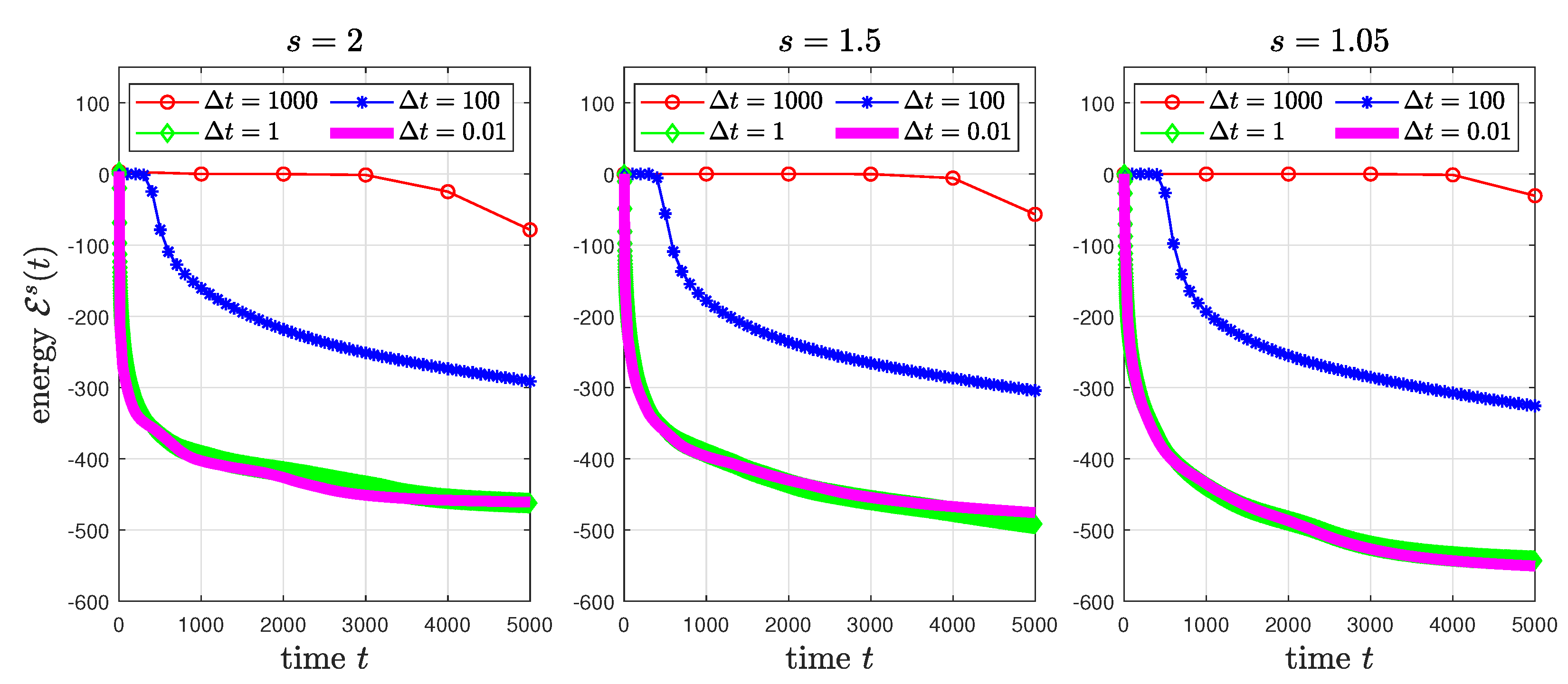
3.1. Accuracy, Efficiency, and Energy Stability Tests

We evolve the solution ϕ ( x , y , t ) of the space-fractional MBE equation from the initial condition [7]
ϕ ( x , y , 0 ) = 0.1 ( sin 3 x sin 2 y + sin 5 x sin 5 y )
on Ω = [ 0 , 2 π ] × [ 0 , 2 π ] . We set δ = 0.1 , h = 2 π / 64 (which provides enough spatial accuracy), and Δ t = 0.01 × 2 9 (which is a sufficiently small time step). For s = 2 , 1.5, and 1.05, Figure 1, Figure 2 and Figure 3 show the evolution of ϕ ( x , y , t ) for 0 < t 30 , respectively. And Figure 4 shows the evolution of energy E s ( t ) and roughness w ( t ) . When s = 2 , the initial modes ( 3 , 2 ) and ( 5 , 5 ) disappear at t = 2.5 . After a buffering time to t = 4 , a new mode ( 1 , 2 ) appears at t = 5.5 . But this unstable mode disappears and only one mode ( 1 , 1 ) is observed in a steady state. This rough–smooth–rough pattern also occurs when s = 1.5 and 1.05. However, it takes a longer buffering time for a new mode to appear as s decreases.
To evaluate the accuracy and efficiency of the proposed method, we perform simulations by varying s = 2 , 1.5 , 1.05 and Δ t = 0.01 · 2 7 , 0.01 · 2 6 , , 0.01 on Intel Core i5-7500 CPU at 3.40 GHz with 8 GB RAM. Figure 5a shows the relative l 2 -errors of ϕ ( x , y , t ) at t = 2.5 and 5.5 for various fractional powers and time steps. Here, the errors are calculated by comparison with the solutions given in Figure 1, Figure 2 and Figure 3. It is observed that the method is second-order accurate in time. And Figure 5b presents the CPU times taken until the last iteration. The results indicate that the CPU time is nearly linear in the number of iterations.
To demonstrate the energy stability and mass conservation of the proposed method, we take much larger time steps. Figure 6 shows the evolution of E s ( t ) and Ω ( ϕ ( x , y , t ) ϕ ( x , y , 0 ) ) d x d y for different fractional powers and time steps. As predicted by Theorem 1, the energy dissipation and mass conservation properties are satisfied even for sufficiently large time steps.

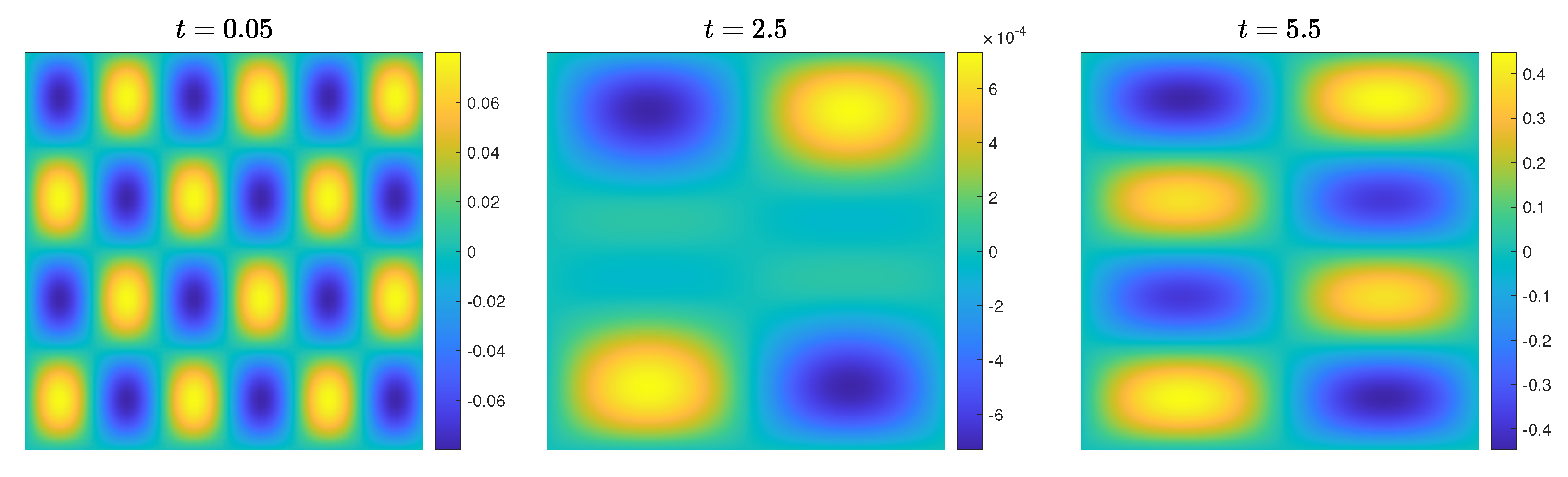
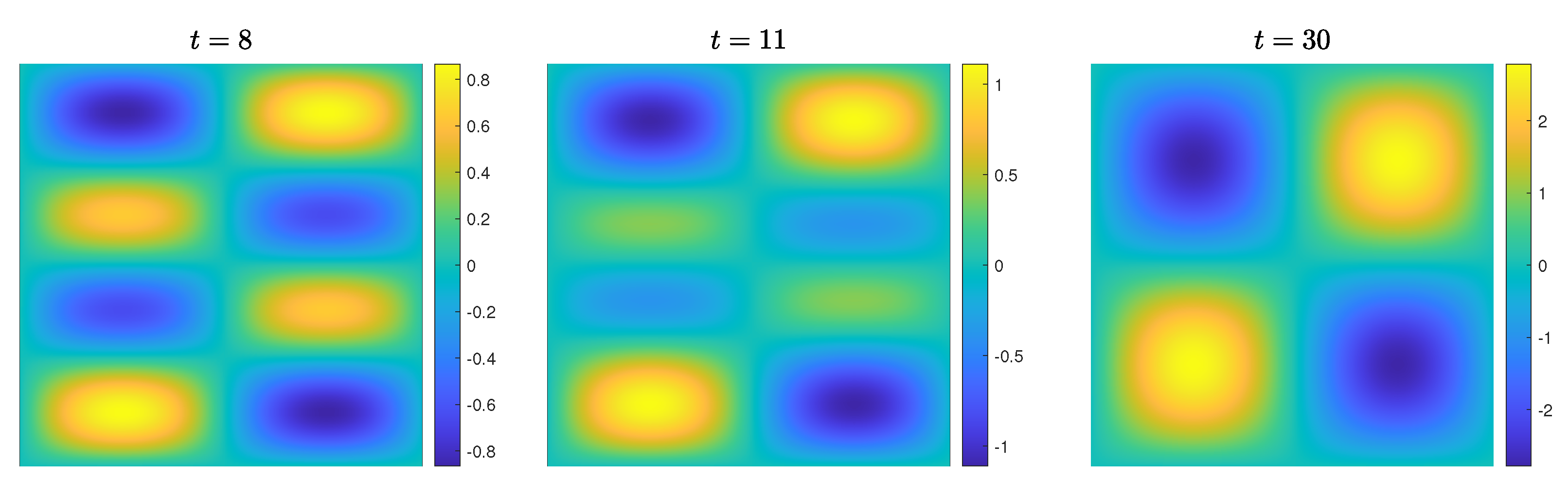
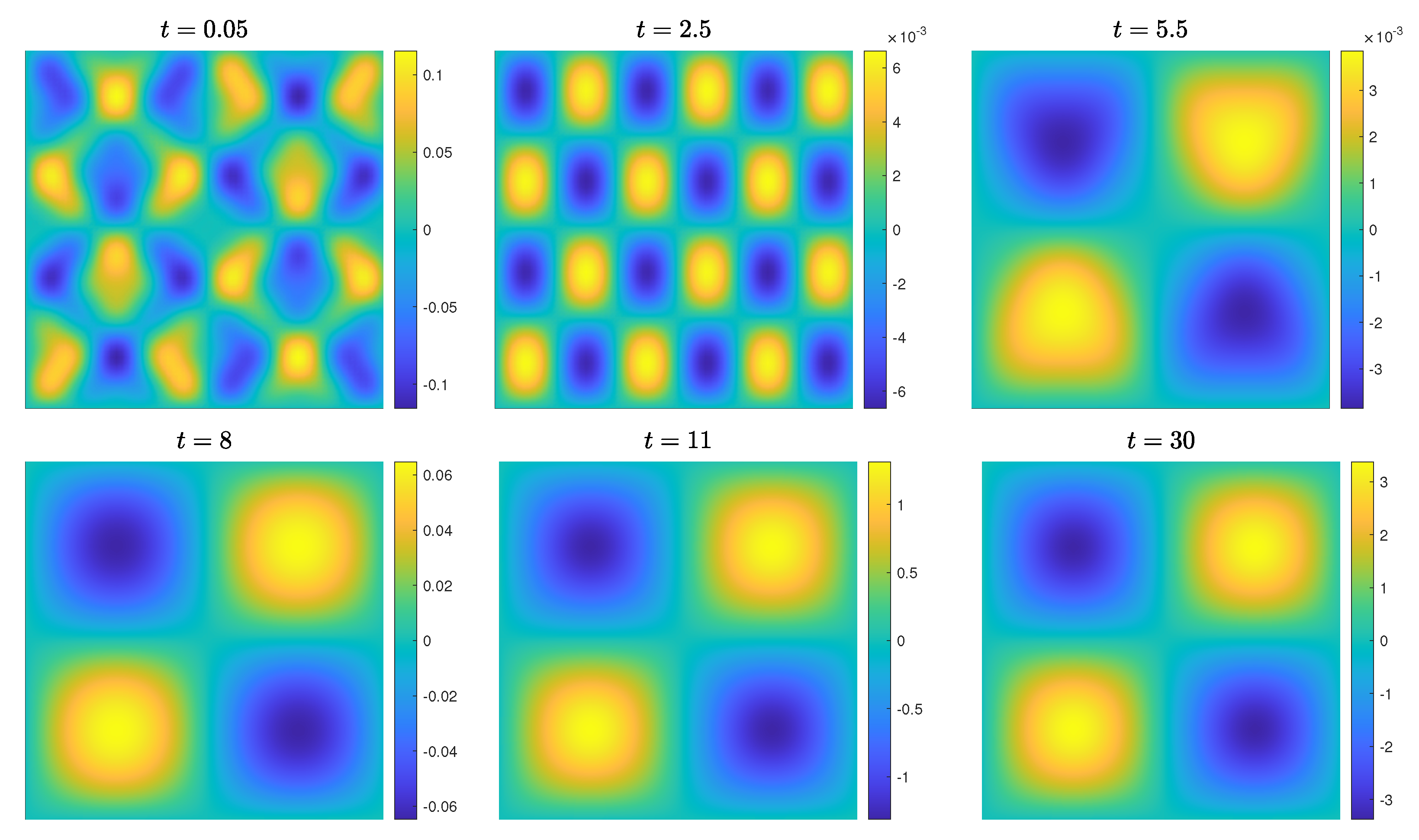
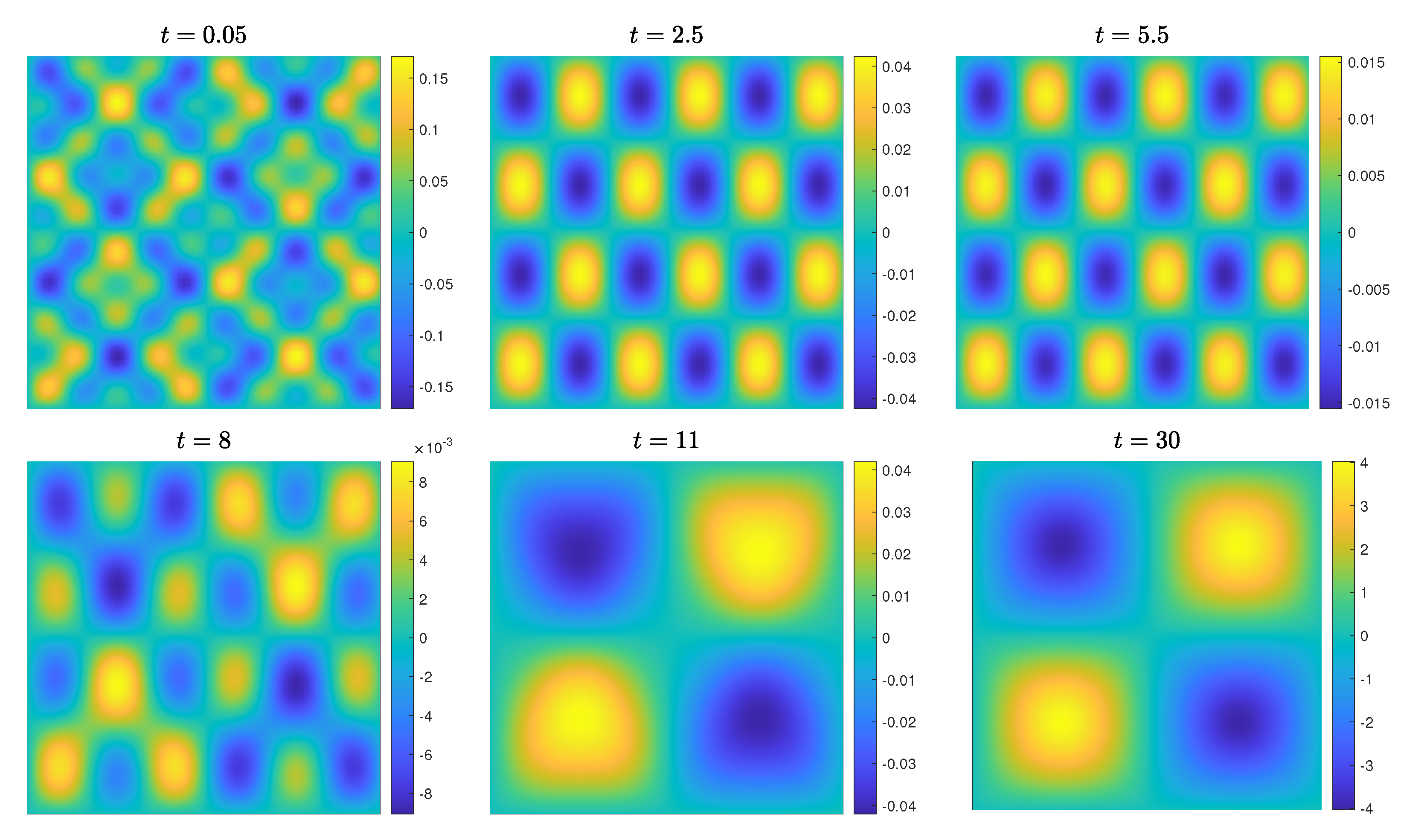
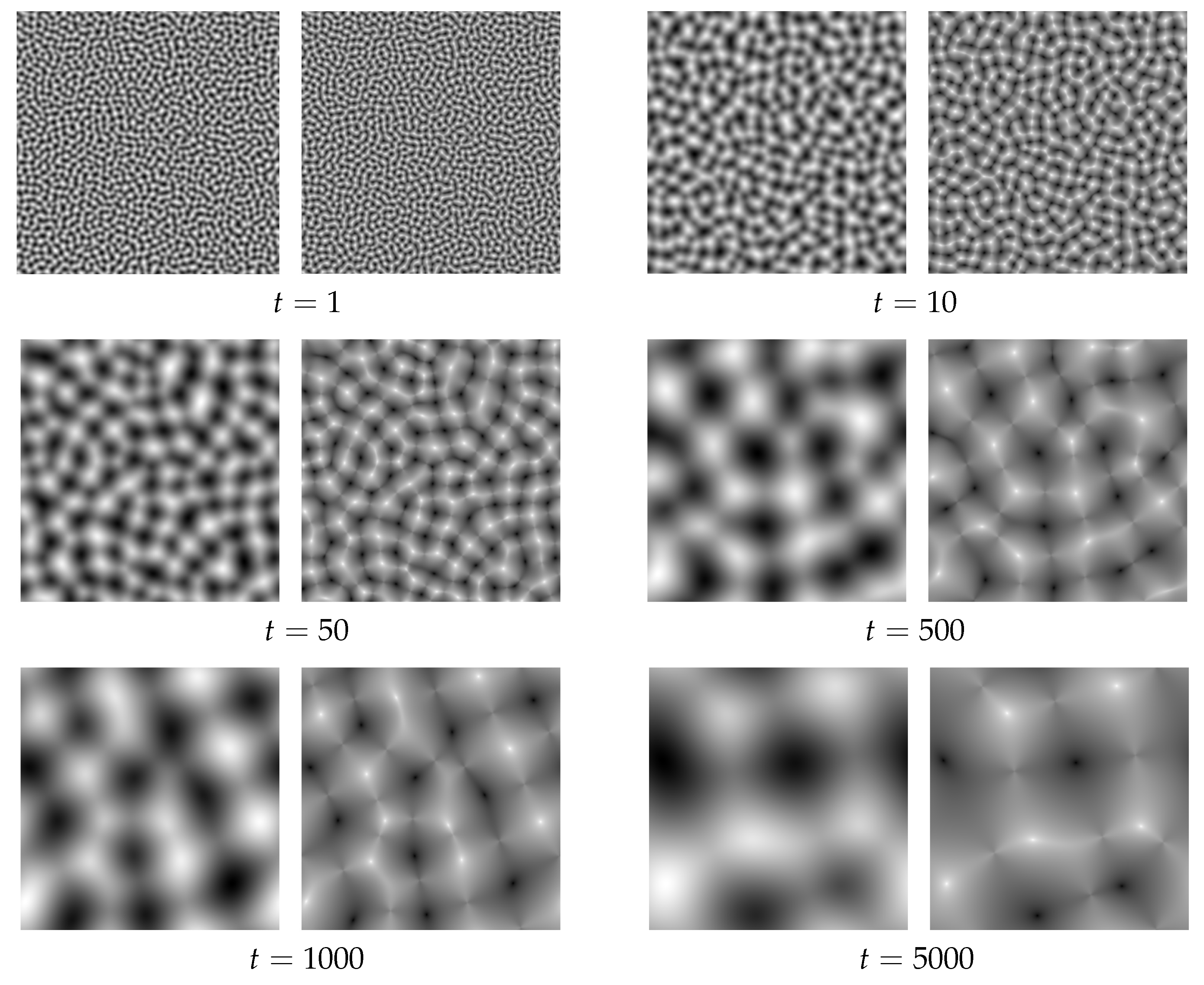
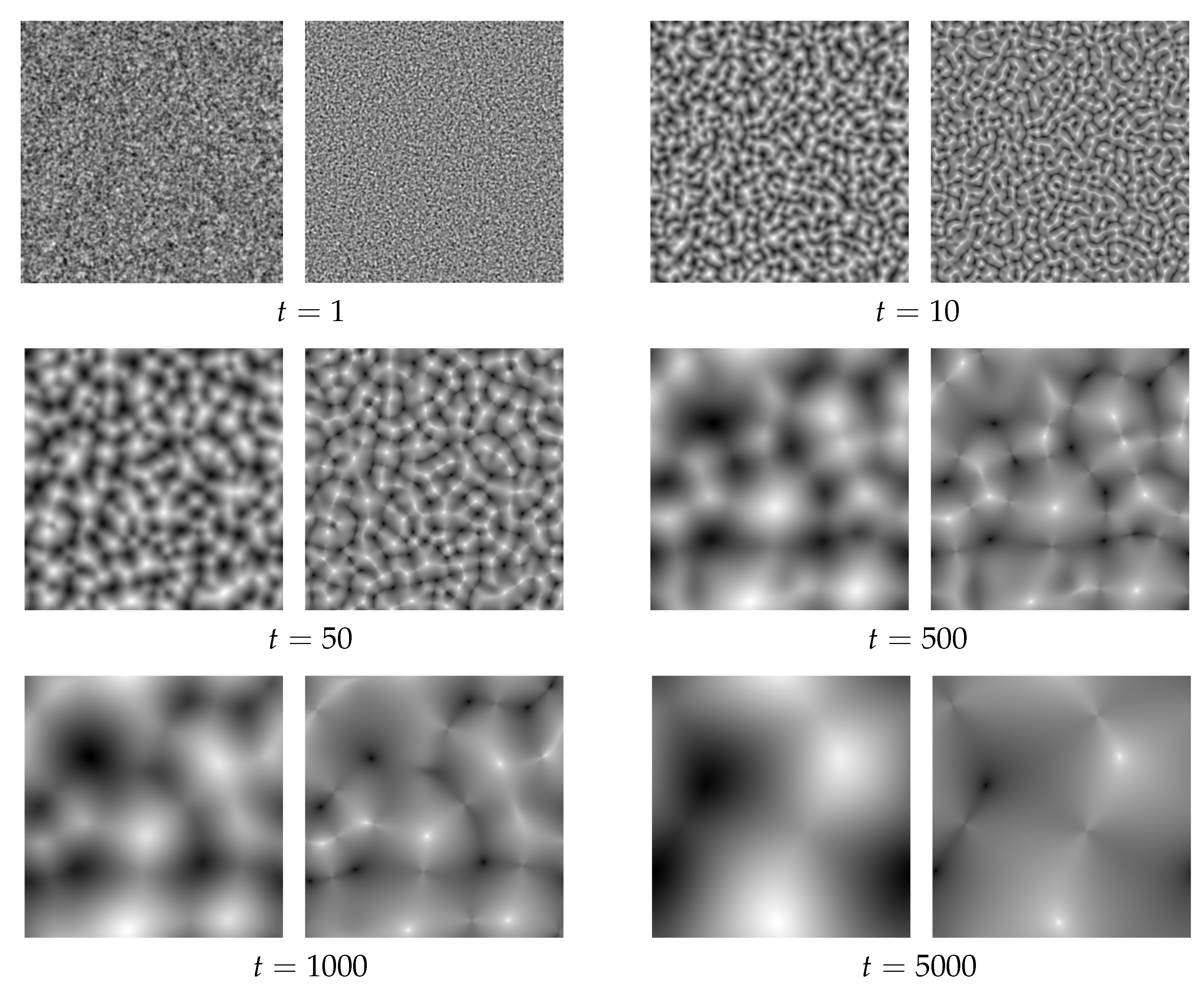
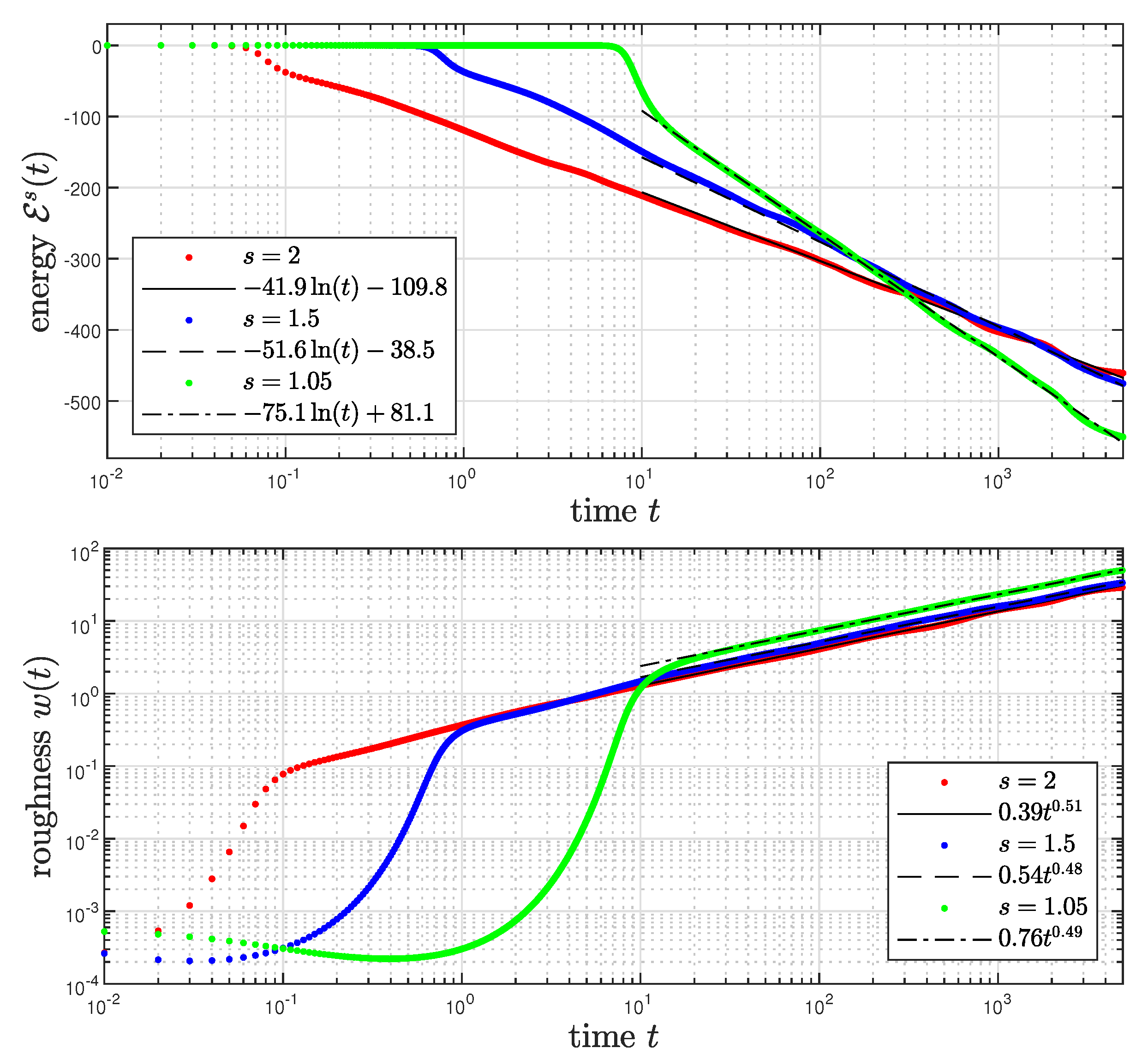
3.2. Coarsening Dynamics

It is known that the classical MBE Equation (2) predicts E ( t ) O ( ln ( t ) ) and w ( t ) O ( t 1 / 2 ) as t [6,7,8,9,10,11,12,13,14,15]. One might wonder whether the fractional power affects the scaling rates. To answer this question numerically, we take an initial condition as ϕ ( x , y , 0 ) = rand ( x , y ) on Ω = [ 0 , 12.8 ] × [ 0 , 12.8 ] , where rand ( x , y ) is a random number between 0.001 and 0.001 at the grid points, and use δ = 0 . 03 2 , h = 12.8 / 512 , and Δ t = 0.01 . For s = 2 , 1.5, and 1.05, Figure 7, Figure 8 and Figure 9 show the evolution of ϕ and its fractional Laplacian ( Δ ) s 2 ϕ for 0 < t 5000 . For all cases, coarsening dynamics with shapes of valleys and hills in the system is obvious. However, the coarsening dynamics goes slower as s decreases at the beginning, but it is much faster after reaching a time point. Figure 10 shows the evolution of E s ( t ) and w ( t ) . The energy decays like ln ( t ) and the roughness grows like t 1 / 2 , with different coefficients dependent upon s. Figure 11 shows the evolution of E s ( t ) for different fractional powers and time steps. The unconditional energy stability of the proposed method is also demonstrated in a long-time simulation.
We also simulate coarsening dynamics in 3D. We take an initial condition as ϕ ( x , y , z , 0 ) = rand ( x , y , z ) on Ω = [ 0 , 3.2 ] × [ 0 , 3.2 ] × [ 0 , 3.2 ] , where rand ( x , y , z ) is a random number between 0.001 and 0.001 at the grid points, and use δ = 0 . 03 2 , h = 3.2 / 128 , and Δ t = 0.01 . Figure 12 shows the evolution of isosurface of ϕ = 0 for various fractional powers. The phenomenon captured in 2D is also observed in 3D.

4. Conclusions

In recent years, the time-fractional MBE model without slope selection has been introduced and solved numerically [32,33,34,35,36,37]. However, it is an open question what a space-fractional generalization of the MBE model without a slope selection is and whether the space-fractional generalization satisfies the energy dissipation and mass conservation properties. This paper was a first attempt to introduce a space-fractional version of the MBE model without slope selection. The numerical idea was not entirely new, but its application to the new energy dissipative system was particularly appropriate since it preserves the original (not modified) energy dissipation law without any assumptions and stabilizers. Our numerical simulations indicated that the energy decays like ln ( t ) and the roughness grows like t 1 / 2 , with different coefficients dependent upon the fractional power.
In future work, we have a plan to carry out rigorous analyses for the well-posedness of the considered problem and for the convergence rate of the proposed method.

Funding

The present research has been conducted by the Research Grant of Kwangwoon University in 2023 and by the National Research Foundation of Korea (NRF) grant funded by the Korea government (MSIT) (No. 2022R1A2C1011708).

Data Availability Statement

Not applicable.

Acknowledgments

The author thanks the reviewers for the constructive and helpful comments on the revision of this article.

Conflicts of Interest

The author declares no conflict of interest.

References

  1. Herman, M.A.; Sitter, H. Molecular Beam Epitaxy: Fundamentals and Current Status; Springer: Berlin/Heidelberg, Germany, 1989. [Google Scholar]
  2. Johnson, M.D.; Orme, C.; Hunt, A.W.; Graff, D.; Sudijono, J.; Sander, L.M.; Orr, B.G. Stable and unstable growth in molecular beam epitaxy. Phys. Rev. Lett. 1994, 72, 116–119. [Google Scholar] [CrossRef] [PubMed]
  3. Ehrlich, G.; Hudda, F.G. Atomic view of surface self-diffusion: Tungsten on tungsten. J. Chem. Phys. 1966, 44, 1039–1049. [Google Scholar] [CrossRef]
  4. Schwoebel, R.L.; Shipsey, E.J. Step motion on crystal surfaces. J. Appl. Phys. 1966, 37, 3682–3686. [Google Scholar] [CrossRef]
  5. Schwoebel, R.L. Step motion on crystal surfaces. II. J. Appl. Phys. 1969, 40, 614–618. [Google Scholar] [CrossRef]
  6. Golubović, L. Interfacial coarsening in epitaxial growth models without slope selection. Phys. Rev. Lett. 1997, 78, 90–93. [Google Scholar] [CrossRef]
  7. Li, B.; Liu, J.-G. Thin film epitaxy with or without slope selection. Eur. J. Appl. Math. 2003, 14, 713–743. [Google Scholar] [CrossRef] [Green Version]
  8. Li, B.; Liu, J.-G. Epitaxial growth without slope selection: Energetics, coarsening, and dynamic scaling. J. Nonlinear Sci. 2004, 14, 429–451. [Google Scholar] [CrossRef] [Green Version]
  9. Chen, W.; Conde, S.; Wang, C.; Wang, X.; Wise, S.M. A linear energy stable scheme for a thin film model without slope selection. J. Sci. Comput. 2012, 52, 546–562. [Google Scholar] [CrossRef]
  10. Yang, X.; Zhao, J.; Wang, Q. Numerical approximations for the molecular beam epitaxial growth model based on the invariant energy quadratization method. J. Comput. Phys. 2017, 333, 104–127. [Google Scholar] [CrossRef] [Green Version]
  11. Li, W.; Chen, W.; Wang, C.; Yan, Y.; He, R. A second order energy stable linear scheme for a thin film model without slope selection. J. Sci. Comput. 2018, 76, 1905–1937. [Google Scholar] [CrossRef]
  12. Ju, L.; Li, X.; Qiao, Z.; Zhang, H. Energy stability and error estimates of exponential time differencing schemes for the epitaxial growth model without slope selection. Math. Comput. 2018, 87, 1859–1885. [Google Scholar] [CrossRef]
  13. Cheng, Q.; Shen, J.; Yang, X. Highly efficient and accurate numerical schemes for the epitaxial thin film growth models by using the SAV approach. J. Sci. Comput. 2019, 78, 1467–1487. [Google Scholar] [CrossRef]
  14. Shin, J.; Lee, H.G. A linear, high-order, and unconditionally energy stable scheme for the epitaxial thin film growth model without slope selection. Appl. Numer. Math. 2021, 163, 30–42. [Google Scholar] [CrossRef]
  15. Kang, Y.; Liao, H.-L.; Wang, J. An energy stable linear BDF2 scheme with variable time-steps for the molecular beam epitaxial model without slope selection. Commun. Nonlinear Sci. Numer. Simul. 2023, 118, 107047. [Google Scholar] [CrossRef]
  16. Barabási, A.-L.; Stanley, H.E. Fractal Concepts in Surface Growth; Cambridge University Press: Cambridge, UK, 1995. [Google Scholar]
  17. Lischke, A.; Pang, G.; Gulian, M.; Song, F.; Glusa, C.; Zheng, X.; Mao, Z.; Cai, W.; Meerschaert, M.M.; Ainsworth, M.; et al. What is the fractional Laplacian? A comparative review with new results. J. Comput. Phys. 2020, 404, 109009. [Google Scholar] [CrossRef]
  18. Liu, F.; Anh, V.; Turner, I. Numerical solution of the space fractional Fokker–Planck equation. J. Comput. Appl. Math. 2004, 166, 209–219. [Google Scholar] [CrossRef] [Green Version]
  19. Meerschaert, M.M.; Tadjeran, C. Finite difference approximations for fractional advection–dispersion flow equations. J. Comput. Appl. Math. 2004, 172, 65–77. [Google Scholar] [CrossRef] [Green Version]
  20. Meerschaert, M.M.; Tadjeran, C. Finite difference approximations for two-sided space-fractional partial differential equations. Appl. Numer. Math. 2006, 56, 80–90. [Google Scholar] [CrossRef]
  21. Ervin, V.J.; Roop, J.P. Variational formulation for the stationary fractional advection dispersion equation. Numer. Meth. Part. Diff. Equ. 2006, 22, 558–576. [Google Scholar] [CrossRef] [Green Version]
  22. Burrage, K.; Hale, N.; Kay, D. An efficient implicit FEM scheme for fractional-in-space reaction-diffusion equations. SIAM J. Sci. Comput. 2012, 34, A2145–A2172. [Google Scholar] [CrossRef] [Green Version]
  23. Wang, F.; Chen, H.; Wang, H. Finite element simulation and efficient algorithm for fractional Cahn–Hilliard equation. J. Comput. Appl. Math. 2019, 356, 248–266. [Google Scholar] [CrossRef]
  24. Zhang, X.; Crawford, J.W.; Deeks, L.K.; Stutter, M.I.; Bengough, A.G.; Young, I.M. A mass balance based numerical method for the fractional advection-dispersion equation: Theory and application. Water Resour. Res. 2005, 41, W07029. [Google Scholar] [CrossRef] [Green Version]
  25. Yang, Q.; Moroney, T.; Burrage, K.; Turner, I.; Liu, F. Novel numerical methods for time-space fractional reaction diffusion equations in two dimensions. ANZIAM J. 2011, 52, C395–C409. [Google Scholar] [CrossRef] [Green Version]
  26. Hejazi, H.; Moroney, T.; Liu, F. Stability and convergence of a finite volume method for the space fractional advection–dispersion equation. J. Comput. Appl. Math. 2014, 255, 684–697. [Google Scholar] [CrossRef] [Green Version]
  27. Weng, Z.; Zhai, S.; Feng, X. A Fourier spectral method for fractional-in-space Cahn–Hilliard equation. Appl. Math. Model. 2017, 42, 462–477. [Google Scholar] [CrossRef]
  28. Bu, L.; Mei, L.; Hou, Y. Stable second-order schemes for the space-fractional Cahn–Hilliard and Allen–Cahn equations. Comput. Math. Appl. 2019, 78, 3485–3500. [Google Scholar] [CrossRef]
  29. Alzahrani, S.M.; Chokri, C. Preconditioned pseudo-spectral gradient flow for computing the steady-state of space fractional Cahn–Allen equations with variable coefficients. Front. Phys. 2022, 10, 844294. [Google Scholar] [CrossRef]
  30. Lee, H.G. A new L2-gradient flow based fractional-in-space modified phase-field crystal equation and its mass conservative and energy stable method. Fractal Fract. 2022, 6, 472. [Google Scholar] [CrossRef]
  31. Li, X.; Han, C.; Wang, Y. Novel patterns in fractional-in-space nonlinear coupled FitzHugh–Nagumo models with Riesz fractional derivative. Fractal Fract. 2022, 6, 136. [Google Scholar] [CrossRef]
  32. Tang, T.; Yu, H.; Zhou, T. On energy dissipation theory and numerical stability for time-fractional phase-field equations. SIAM J. Sci. Comput. 2019, 41, A3757–A3778. [Google Scholar] [CrossRef] [Green Version]
  33. Zhao, J.; Chen, L.; Wang, H. On power law scaling dynamics for time-fractional phase field models during coarsening. Commun. Nonlinear Sci. Numer. Simul. 2019, 70, 257–270. [Google Scholar] [CrossRef] [Green Version]
  34. Ji, B.; Liao, H.-L.; Gong, Y.; Zhang, L. Adaptive second-order Crank–Nicolson time-stepping schemes for time-fractional molecular beam epitaxial growth models. SIAM J. Sci. Comput. 2020, 42, B738–B760. [Google Scholar] [CrossRef]
  35. Hou, D.; Xu, C. Robust and stable schemes for time fractional molecular beam epitaxial growth model using SAV approach. J. Comput. Phys. 2021, 445, 110628. [Google Scholar] [CrossRef]
  36. Zhu, X.; Liao, H.-L. Asymptotically compatible energy law of the Crank–Nicolson type schemes for time-fractional MBE models. Appl. Math. Lett. 2022, 134, 108337. [Google Scholar] [CrossRef]
  37. Wang, J.; Yang, Y.; Ji, B. Two energy stable variable-step L1 schemes for the time-fractional MBE model without slope selection. J. Comput. Appl. Math. 2023, 419, 114702. [Google Scholar] [CrossRef]
  38. Kim, J.; Lee, H.G. Unconditionally energy stable second-order numerical scheme for the Allen–Cahn equation with a high-order polynomial free energy. Adv. Differ. Equ. 2021, 2021, 416. [Google Scholar] [CrossRef]
  39. Lee, H.G. A non-iterative and unconditionally energy stable method the Swift–Hohenberg equation with quadratic–cubic nonlinearity. Appl. Math. Lett. 2022, 123, 107579. [Google Scholar] [CrossRef]
  40. Lee, H.G.; Shin, J.; Lee, J.-Y. A high-order and unconditionally energy stable scheme for the conservative Allen–Cahn equation with a nonlocal Lagrange multiplier. J. Sci. Comput. 2022, 90, 51. [Google Scholar] [CrossRef]
  41. Lee, H.G.; Shin, J.; Lee, J.-Y. Energy quadratization Runge–Kutta scheme for the conservative Allen–Cahn equation with a nonlocal Lagrange multiplier. Appl. Math. Lett. 2022, 132, 108161. [Google Scholar] [CrossRef]
  42. Lee, H.G. Stability condition of the second-order SSP-IMEX-RK method for the Cahn–Hilliard equation. Mathematics 2020, 8, 11. [Google Scholar] [CrossRef] [Green Version]
Figure 1. Evolution of ϕ ( x , y , t ) with s = 2 and δ = 0.1 .
Fractalfract 07 00558 g001aFractalfract 07 00558 g001b
Figure 2. Evolution of ϕ ( x , y , t ) with s = 1.5 and δ = 0.1 .
Fractalfract 07 00558 g002
Figure 3. Evolution of ϕ ( x , y , t ) with s = 1.05 and δ = 0.1 .
Fractalfract 07 00558 g003
Figure 4. Evolution of E s ( t ) (top) and w ( t ) (bottom) with δ = 0.1 .
Fractalfract 07 00558 g004
Figure 5. (a) Relative l 2 -errors of ϕ ( x , y , t ) at t = 2.5 and 5.5 and (b) CPU times taken until the last iteration for various fractional powers and time steps.
Fractalfract 07 00558 g005
Figure 6. Evolution of (a) E s ( t ) and (b) Ω ( ϕ ( x , y , t ) ϕ ( x , y , 0 ) ) d x d y for different fractional powers and time steps.
Fractalfract 07 00558 g006
Figure 7. Evolution of ϕ (left) and its fractional Laplacian ( Δ ) s 2 ϕ (right) with s = 2 and δ = 0 . 03 2 .
Fractalfract 07 00558 g007
Figure 8. Evolution of ϕ (left) and its fractional Laplacian ( Δ ) s 2 ϕ (right) with s = 1.5 and δ = 0 . 03 2 .
Fractalfract 07 00558 g008
Figure 9. Evolution of ϕ (left) and its fractional Laplacian ( Δ ) s 2 ϕ (right) with s = 1.05 and δ = 0 . 03 2 .
Fractalfract 07 00558 g009
Figure 10. Evolution of E s ( t ) (top) and w ( t ) (bottom) with δ = 0 . 03 2 . The dots represent the results obtained by the simulation, while the solid, dashed, and dash-dotted lines are obtained by least squares fitting of the results.
Fractalfract 07 00558 g010
Figure 11. Evolution of E s ( t ) for different fractional powers and time steps.
Fractalfract 07 00558 g011
Figure 12. Evolution of isosurface of ϕ = 0 with (a) s = 2 , (b) 1.5, and (c) 1.05. Times are t = 1 , 5, 10, and 100 (from left to right).
Fractalfract 07 00558 g012
Disclaimer/Publisher’s Note: The statements, opinions and data contained in all publications are solely those of the individual author(s) and contributor(s) and not of MDPI and/or the editor(s). MDPI and/or the editor(s) disclaim responsibility for any injury to people or property resulting from any ideas, methods, instructions or products referred to in the content.

