Similarity Reductions, Power Series Solutions, and Conservation Laws of the Time-Fractional Mikhailov–Novikov–Wang System

Abstract

The current study presents a comprehensive Lie symmetry analysis for the time-fractional Mikhailov–Novikov–Wang (MNW) system with the Riemann–Liouville fractional derivative. The corresponding simplified equations with the Erdélyi–Kober fractional derivative are constructed by group invariant solutions. Furthermore, we obtain explicit solutions with the help of the power series method and show the dynamical behavior via evolutional figures. Finally, by means of Ibragimov’s new conservation theorem, the conservation laws are derived for the system.

1. Introduction

Over the last few decades, many researchers have focused on analyzing the propagation of nonlinear waves on the ocean surface found in various areas, including ocean engineering, plasma, hydrodynamics, and tsunami waves. In 1871, Boussinesq [1] presented a model that explained the propagation of long waves in shallow water. This model has significant applications in the numerical simulation of nonlinear string vibration, plasma acoustic waves, coastal engineering, and shallow water waves [2]. In 2006, Mikhailov, Novikov, and Wang [3] proposed a productively extended Boussinesq equation known as the Mikhailov–Novikov–Wang equation

$$u_{tt}-u_{xxxt}-8u_x{u}_{xt}-4u_{xx}{u}_t+2u_x{u}_{xxxx}+4u_{xx}{u}_{xxx}+24u_x^2{u}_{xx}=0.$$

(1)

This is an integrable equation with dynamical behavior, and studying the solutions of this model can help to understand many interesting nonlinear scientific phenomena [4]. Raza and others [5] used the singular manifold method, spread method, and generalized projective Riccati equation method to acquire hyperbolic and trigonometric solutions of the equation. Ray S et al. [6] employed the simplified Hirota method to examine the twisted multiple soliton solutions and provided a graphical representation of the findings. Additionally, Ray S [7] also utilized the Lie symmetry method to obtain similarity reductions, conservation laws, and explicit exact solutions. Similarly, Demiray et al. [8] used the GERFM method to solve the MNW equation and obtained trigonometric, hyperbolic, and dark soliton solutions.

In the literature [3], Mikhailov and others introduced the MNW equation and revealed a fully integrable fifth-order nonlinear partial differential system called the MNW system

$$\left\{\begin{array}{c}\begin{array}{c}{u}_t=u_{xxxxx}-20u{u}_{xxx}-50u_x{u}_{xx}+80u^2{u}_x+v_x,\hfill \\ v_t=-6v{u}_{xxx}-2u_{xx}{v}_x+96vu{u}_x+16v_x{u}^2,\hfill \end{array}\end{array}\right.$$

(2)

where the velocity function $u(x,t)$ and the height function $v(x,t)$ are differentiable functions. Sergyeyev [9] presented a zero curvature representation of the MNW system in their paper and constructed multiple solitons and finite gap solutions using inverse scattering transformations. Sierra [10] obtained the traveling wave solutions of the MNW system via the extended tanh method. Similarly, ref. [11] applied the same methodology to obtain solitary waves and periodic and soliton solutions of the system. Shan and others [12] used the Lie algebra approach to demonstrate that the equations are integrable in the Lax sense and possess Hamiltonian structures.

To date, research on the MNW system has only been considered integer orders. We will study the system in time-fractional order to enable a more comprehensive study of the MNW system

$$\left\{\begin{array}{c}\begin{array}{c}{D}_t^{\alpha }u=a_1{u}_{xxxxx}+a_{2}u{u}_{xxx}+a_3{u}_x{u}_{xx}+a_4{u}^2{u}_x+a_5{v}_x,\hfill \\ D_t^{\alpha }v=b_{1}v{u}_{xxx}+b_2{u}_{xx}{v}_x+b_{3}vu{u}_x+b_4{v}_x{u}^2,\hfill \end{array}\end{array}\right.$$

(3)

where $0<\alpha ⩽1$, $D_t^{\alpha }$ denotes the Riemann–Liouville derivative operator, and $a_i$, $b_j$, $i=1\cdots 5$, $j=1\cdots 4$ are constants. The time-fractional MNW system is a new system that scholars have not studied before. When we take $\alpha =1$, the system (3) degenerates into the MNW system, a Boussinesq-type integrable system that describes nonlinear wave phenomena. The time-fractional MNW system is an extension of the MNW system in time, and it can be used to simulate the dynamic behavior of water wave propagation in oceanography and atmospheric science. Therefore, it is vital to investigate its properties and explicit solutions.

The fractional partial differential equation (FPDE) has garnered considerable attention due to its broad usage in scientific and engineering fields [13,14,15]. It represents natural phenomena more accurately than the integer partial differential equation. Therefore, finding effective methods to study the FPDE is of great significance [16]. To date, numerical and analytical methods exist for solving the FPDE, including the finite difference method [17,18], the homotopy analysis method [19], the sub-equation method [20,21], the invariant subspace method [22,23,24], the Lie symmetry analysis method [25,26,27,28,29], and so on. Lie symmetry analysis, in particular, offers a powerful technique for solving partial differential equations and can yield vital symmetry properties such as invariant solutions and conservation laws [30]. Implementing group invariant solutions can facilitate the discovery of additional invariant subspaces about the relevant differential operators while reducing the original equations’ complexity. Meanwhile, conservation laws play a critical role in examining differential equations’ properties and verifying the solutions’ precision and stability. In 2007, Gazizov et al. [31,32] extended Lie symmetry analysis to FPDEs, then some researchers applied the Lie group method to study the FPDE and obtained many vital solutions.

This study aims to use the Lie symmetry analysis method to solve the time-fractional MNW system and present the conservation laws of the system by Ibragimov’s new conservation theorem.

The remaining sections of this paper are structured as follows: Section 2 presents the definition and property of the Riemann–Liouville fractional derivative. In the next section, we introduce the application of classical Lie group theory to the time-fractional partial differential system. The focus of Section 4 is to apply Lie symmetry theory to our fractional MNW system to obtain Lie symmetry generating elements and the reduced system. Next, Section 5 uses the power series method to solve the time-fractional ordinary differential equations and analyze the solution’s convergence. In Section 6, we establish the non-local conservation laws separately for each of the obtained Lie symmetries according to Ibragimov’s new conservation theorem. Section 7 discusses the dynamical behavior of the newly discovered power series solutions. Finally, the concluding remarks of this paper are presented in the last section.

2. Definition and Properties of the Riemann–Liouville Fractional Derivative

It is well known that there are various definitions of fractional derivatives, such as Riemann–Liouville type, Caputo type, Weyl type, etc. In our research, we adopt the Riemann–Liouville fractional derivative:

$${}_a{D}_t^{\alpha }f(t,x)=D_t^n{}_a{I}_t^{n-\alpha }f(t,x)=\left\{\begin{array}{c}\begin{array}{c}\frac{1}{\mathsf{\Gamma }(n-\alpha )}\frac{{\partial }^n}{\partial t^n}{\int }_a^t\frac{f(\tau ,x)}{{(t-\tau )}^{\alpha +1-n}}d\tau ,n-1<\alpha <n,n\in N,\hfill \\ D_t^{n}f(t,x),\alpha =n\in N,\hfill \end{array}\end{array}\right.$$

(4)

where $t>a$, and we denote the operator ${}_o{D}_t^{\alpha }$ as $D_t^{\alpha }$ throughout this paper.

The properties of the fractional derivative are

$$D^{\alpha }{t}^{\beta }=\frac{\mathsf{\Gamma }(\beta +1)t^{\beta -\alpha }}{\mathsf{\Gamma }(\beta -\alpha +1)},\beta >\alpha -1.$$

(5)

3. Lie Symmetry Analysis for the Time-Fractional Partial Differential System

Applying Lie symmetry group theory to the fractional partial differential system is essential for comprehensively comprehending our system’s mathematical and physical meaning. Let us provide a concise overview of fundamental concepts and derive the formula for the $\alpha$-th extended infinitesimal of the Riemann–Liouville time-fractional derivative, which distinctly differs from the integer order states.

Consider a time-fractional partial differential system with independent variables of x and t as follows

$$\left\{\begin{array}{c}\begin{array}{c}{D}_t^{\alpha }u=F\left(x,t,u,u_t,u_x,u_{xx},u_{xxx},u_{xxxxx},v,v_t,v_x\right),\hfill \\ D_t^{\alpha }v=G\left(x,t,u,u_t,u_x,u_{xx},u_{xxx},v,v_t,v_x\right).\hfill \end{array}\end{array}\right.$$

(6)

Assume the system (6) is invariant under the one-parameter $\left(\epsilon \right)$ Lie infinitesimal transformation group

$$\begin{array}{cc}\hfill x^{*}\hfill & \hfill =x+\epsilon \xi (x,t,u,v)+O\left({\epsilon }^2\right),\hfill \\ \hfill t^{*}\hfill & \hfill =t+\epsilon \tau (x,t,u,v)+O\left({\epsilon }^2\right),\hfill \\ \hfill u^{*}\hfill & \hfill =u+\epsilon \eta (x,t,u,v)+O\left({\epsilon }^2\right),\hfill \\ \hfill v^{*}\hfill & \hfill =v+\epsilon \varphi (x,t,u,v)+O\left({\epsilon }^2\right),\hfill \\ \hfill \frac{{\partial }^{\alpha }{u}^{*}}{\partial t^{*\alpha }}\hfill & \hfill =\frac{{\partial }^{\alpha }u}{\partial t^{\alpha }}+\epsilon {\eta }_t^{\alpha }(x,t,u,v)+O\left({\epsilon }^2\right),\hfill \\ \hfill \frac{{\partial }^{\alpha }{v}^{*}}{\partial t^{*\alpha }}\hfill & \hfill =\frac{{\partial }^{\alpha }v}{\partial t^{\alpha }}+\epsilon {\varphi }_t^{\alpha }(x,t,u,v)+O\left({\epsilon }^2\right),\hfill \\ \hfill \frac{\partial u^{*}}{\partial x^{*}}\hfill & \hfill =\frac{\partial u}{\partial x}+\epsilon {\eta }^x(x,t,u,v)+O\left({\epsilon }^2\right),\hfill \\ \hfill \frac{\partial v^{*}}{\partial x^{*}}\hfill & \hfill =\frac{\partial v}{\partial x}+\epsilon {\varphi }^x(x,t,u,v)+O\left({\epsilon }^2\right),\hfill \\ \hfill \frac{{\partial }^2{u}^{*}}{\partial x^{*2}}\hfill & \hfill =\frac{{\partial }^{2}u}{\partial x^2}+\epsilon {\eta }^{xx}(x,t,u,v)+O\left({\epsilon }^2\right),\hfill \\ \hfill \frac{{\partial }^3{u}^{*}}{\partial x^{*3}}\hfill & \hfill =\frac{{\partial }^{3}u}{\partial x^3}+\epsilon {\eta }^{xxx}(x,t,u,v)+O\left({\epsilon }^2\right),\hfill \\ \hfill \frac{{\partial }^5{u}^{*}}{\partial x^{*5}}\hfill & \hfill =\frac{{\partial }^{5}u}{\partial x^5}+\epsilon {\eta }^{xxxxx}(x,t,u,v)+O\left({\epsilon }^2\right),\hfill \end{array}$$

(7)

where $\epsilon \ll 1$ is a group parameter and $\xi$, $\tau$, $\eta$, and $\varphi$ are infinitesimals. Now, we give several extended infinitesimals

$$\begin{array}{c}{\eta }^x=D_x\left(\eta \right)-u_x{D}_x\left(\xi \right)-u_t{D}_x\left(\tau \right),\\ {\varphi }^x=D_x\left(\varphi \right)-v_x{D}_x\left(\xi \right)-v_t{D}_x\left(\tau \right),\\ {\eta }^{xx}=D_x\left({\eta }^x\right)-u_{xx}{D}_x\left(\xi \right)-u_{xt}{D}_x\left(\tau \right),\\ {\eta }^{xxx}=D_x\left({\eta }^{xx}\right)-u_{xxx}{D}_x\left(\xi \right)-u_{xxt}{D}_x\left(\tau \right),\\ {\eta }^{xxxxx}=D_x\left({\eta }^{xxxx}\right)-u_{xxxxx}{D}_x\left(\xi \right)-u_{xxxxt}{D}_x\left(\tau \right),\end{array}$$

(8)

where the total derivatives of x and t are denoted as $D_x$ and $D_t$ and defined as

$$D_{x^k}=\frac{\partial }{\partial x^k}+u_k\frac{\partial }{\partial u}+v_k\frac{\partial }{\partial v}+u_{kj}\frac{\partial }{\partial u_j}+v_{kj}\frac{\partial }{\partial u_j}+···,j=1,2,$$

where $x^k$ can be considered for both independent variables x and t as $x^1=x$, $x^2=t$.

The infinite generator V associated with the above group transformations is as follows

$$V=\xi \left(x,t,u,v\right)\frac{\partial }{\partial x}+\tau \left(x,t,u,v\right)\frac{\partial }{\partial t}+\eta \left(x,t,u,v\right)\frac{\partial }{\partial u}+\varphi \left(x,t,u,v\right)\frac{\partial }{\partial v}.$$

(9)

It is necessary to construct the invariance conditions of the system (6) under the point transformations of Equation (7)

$$\left\{\begin{array}{c}{\left.p{r}^{(\alpha ,5)}V\left({\Delta }_1\right)\right|}_{{\Delta }_1=0}=0,\hfill \\ {\left.p{r}^{(\alpha ,3)}V\left({\Delta }_2\right)\right|}_{{\Delta }_2=0}=0,\hfill \end{array}\right.$$

(10)

where

$$\left\{\begin{array}{c}{\Delta }_1=D_t^{\alpha }u-F\left(x,t,u,u_t,u_x,u_{xx},u_{xxx},u_{xxxxx},v,v_t,v_x\right),\hfill \\ {\Delta }_2=D_t^{\alpha }v-G\left(x,t,u,u_t,u_x,u_{xx},u_{xxx},v,v_t,v_x\right).\hfill \end{array}\right.$$

As the lower limit of the integral in system (6) remains fixed, it maintains invariance under the transformations outlined in Equation (7). Thus, the corresponding invariance condition [33] becomes

$${\left.\tau (x,t,u,v)\right|}_{t=0}=0.$$

(11)

The ${\eta }_t^{\alpha }$ and ${\varphi }_t^{\alpha }$ are the $\alpha$-th extended infinitesimal related to the Riemann–Liouville time-fractional derivative

$$\left\{\begin{array}{c}{\eta }_t^{\alpha }=D_t^{\alpha }\left(\eta \right)+\xi D_t^{\alpha }\left(u_x\right)-D_t^{\alpha }\left(\xi u_x\right)+D_t^{\alpha }\left(D_t\left(\tau \right)u\right)-D_t^{\alpha +1}\left(\tau u\right)+\tau D_t^{\alpha +1}\left(u\right),\hfill \\ {\varphi }_t^{\alpha }=D_t^{\alpha }\left(\varphi \right)+\xi D_t^{\alpha }\left(v_x\right)-D_t^{\alpha }\left(\xi v_x\right)+D_t^{\alpha }\left(D_t\left(\tau \right)v\right)-D_t^{\alpha +1}\left(\tau v\right)+\tau D_t^{\alpha +1}\left(v\right),\hfill \end{array}\right.$$

(12)

where the character $D_t^{\alpha }$ represents the total time-fractional derivative operator.

To simplify Equation (12), we need the generalized Leibniz formula in the fractional sense

$$D_t^{\alpha }\left[f\left(t\right)g\left(t\right)\right]=\sum _{j=0}^{\infty }\left(\begin{array}{c}\alpha \\ j\end{array}\right)D_t^{\alpha -j}f\left(t\right)D_t^{j}g\left(t\right),\alpha >0,$$

(13)

where $\left(\begin{array}{c}\alpha \hfill \\ j\hfill \end{array}\right)=\frac{{(-1)}^{j-1}\alpha \mathsf{\Gamma }(j-\alpha )}{\mathsf{\Gamma }(1-\alpha )\mathsf{\Gamma }(j+1)}$.

Substituting Equation (13) into the system (12), the following expression is obtained

$$\left\{\begin{array}{c}\begin{array}{cc}\hfill {\eta }_t^{\alpha }& =D_t^{\alpha }\left(\eta \right)-\alpha D_t\left(\tau \right)\frac{{\partial }^{\alpha }u}{\partial t^{\alpha }}\hfill \\ \hfill & -\sum _{m=1}^{\infty }\left(\begin{array}{c}\alpha \\ m\end{array}\right)D_t^m\left(\xi \right)D_t^{\alpha -m}{u}_x-\sum _{m=1}^{\infty }\left(\begin{array}{c}\alpha \\ m+1\end{array}\right)D_t^{m+1}\left(\tau \right)D_t^{\alpha -m}\left(u\right),\hfill \end{array}\hfill \\ \begin{array}{cc}\hfill {\varphi }_t^{\alpha }& =D_t^{\alpha }\left(\varphi \right)-\alpha D_t\left(\tau \right)\frac{{\partial }^{\alpha }v}{\partial t^{\alpha }}\hfill \\ \hfill & -\sum _{m=1}^{\infty }\left(\begin{array}{c}\alpha \hfill \\ m\hfill \end{array}\right)D_t^m\left(\xi \right)D_t^{\alpha -m}{v}_x-\sum _{m=1}^{\infty }\left(\begin{array}{c}\alpha \\ m+1\end{array}\right)D_t^{m+1}\left(\tau \right)D_t^{\alpha -m}\left(v\right).\hfill \end{array}\hfill \end{array}\right.$$

(14)

On the other hand, we review the generalized chain rule for composite functions in this form

$$\frac{d^{m}g\left[f\left(t\right)\right]}{d{t}^m}=\sum _{j=0}^m\sum _{r=0}^j\left(\begin{array}{c}j\hfill \\ r\hfill \end{array}\right)\frac{1}{j!}{[-f\left(t\right)]}^r\frac{d^m}{d{t}^m}\left[f{\left(t\right)}^{j-r}\right]\frac{d^{j}g\left(f\right)}{d{f}^j}.$$

(15)

Applying the chain rule (15) and the generalized Leibniz formula (13), let $f\left(t\right)=1$. Then, the expression for $D_t^{\alpha }\left(\eta \right)$ and $D_t^{\alpha }\left(\varphi \right)$ in Equation (14) becomes

$$\left\{\begin{array}{c}{\displaystyle D_t^{\alpha }\left(\eta \right)=\frac{{\partial }^{\alpha }\eta }{\partial t^{\alpha }}+{\eta }_u\frac{{\partial }^{\alpha }u}{\partial t^{\alpha }}-u\frac{{\partial }^{\alpha }{\eta }_u}{\partial t^{\alpha }}+\sum _{m=1}^{\infty }\left(\begin{array}{c}\alpha \hfill \\ m\hfill \end{array}\right)\frac{{\partial }^m{\eta }_u}{\partial t^m}{D}_t^{\alpha -m}\left(u\right)+\delta ,}\hfill \\ {\displaystyle D_t^{\alpha }\left(\varphi \right)=\frac{{\partial }^{\alpha }\varphi }{\partial t^{\alpha }}+{\varphi }_v\frac{{\partial }^{\alpha }v}{\partial t^{\alpha }}-v\frac{{\partial }^{\alpha }{\varphi }_v}{\partial t^{\alpha }}+\sum _{m=1}^{\infty }\left(\begin{array}{c}\alpha \hfill \\ m\hfill \end{array}\right)\frac{{\partial }^m{\varphi }_v}{\partial t^m}{D}_t^{\alpha -m}\left(v\right)+\omega ,}\hfill \end{array}\right.$$

(16)

where

$$\left\{\begin{array}{c}{\displaystyle \delta =\sum _{m=2}^{\infty }\sum _{n=2}^m\sum _{j=2}^n\sum _{r=0}^{j-1}\left(\begin{array}{c}\alpha \hfill \\ m\hfill \end{array}\right)\left(\begin{array}{c}m\hfill \\ n\hfill \end{array}\right)\left(\begin{array}{c}j\hfill \\ r\hfill \end{array}\right)\frac{1}{j!}\frac{t^{m-\alpha }}{\mathsf{\Gamma }(m+1-\alpha )}{(-u)}^r\frac{{\partial }^n}{\partial t^n}\left(u^{j-r}\right)\frac{{\partial }^{m-n+j}\eta }{\partial t^{m-n}\partial u^j},}\hfill \\ {\displaystyle \omega =\sum _{m=2}^{\infty }\sum _{n=2}^m\sum _{j=2}^n\sum _{r=0}^{j-1}\left(\begin{array}{c}\alpha \hfill \\ m\hfill \end{array}\right)\left(\begin{array}{c}m\hfill \\ n\hfill \end{array}\right)\left(\begin{array}{c}j\hfill \\ r\hfill \end{array}\right)\frac{1}{j!}\frac{t^{m-\alpha }}{\mathsf{\Gamma }(m+1-\alpha )}{(-v)}^r\frac{{\partial }^n}{\partial t^n}\left(v^{j-r}\right)\frac{{\partial }^{m-n+j}\varphi }{\partial t^{m-n}\partial v^j}.}\hfill \end{array}\right.$$

Thus, the explicit form of Equation (14) becomes

$$\left\{\begin{array}{cc}{\eta }_t^{\alpha }\hfill & =\frac{{\partial }^{\alpha }\eta }{\partial t^{\alpha }}+\left({\eta }_u-\alpha D_t\left(\tau \right)\right)\frac{{\partial }^{\alpha }u}{\partial t^{\alpha }}-u\frac{{\partial }^{\alpha }{\eta }_u}{\partial t^{\alpha }}+\delta \hfill \\ \hfill & +\sum _{m=1}^{\infty }\left[\left(\begin{array}{c}\alpha \\ m\end{array}\right)\frac{{\partial }^{\alpha }{\eta }_u}{\partial t^{\alpha }}-\left(\begin{array}{c}\alpha \\ m+1\end{array}\right)D_t^{m+1}\left(\tau \right)\right]D_t^{\alpha -m}\left(u\right)-\sum _{m=1}^{\infty }\left(\begin{array}{c}\alpha \\ m\end{array}\right)D_t^m\left(\xi \right)D_t^{\alpha -m}{u}_x,\hfill \\ {\varphi }_t^{\alpha }\hfill & =\frac{{\partial }^{\alpha }\varphi }{\partial t^{\alpha }}+\left({\varphi }_v-\alpha D_t\left(\tau \right)\right)\frac{{\partial }^{\alpha }v}{\partial t^{\alpha }}-v\frac{{\partial }^{\alpha }{\varphi }_v}{\partial t^{\alpha }}+\omega \hfill \\ \hfill & +\sum _{m=1}^{\infty }\left[\left(\begin{array}{c}\alpha \\ m\end{array}\right)\frac{{\partial }^{\alpha }{\varphi }_v}{\partial t^{\alpha }}-\left(\begin{array}{c}\alpha \\ m+1\end{array}\right)D_t^{m+1}\left(\tau \right)\right]D_t^{\alpha -m}\left(v\right)-\sum _{m=1}^{\infty }\left(\begin{array}{c}\alpha \\ m\end{array}\right)D_t^m\left(\xi \right)D_t^{\alpha -m}{v}_x.\hfill \end{array}\right.$$

(17)

4. Lie Symmetry Analysis and Reduction

In the preceding section, we provided an overview of the preparatory work for utilizing the Lie symmetry method when dealing with the time-fractional partial differential system. In this section, we will apply the above Lie theory to present group invariant solutions and reduced systems for the time-fractional MNW system.

Calculating

$$\left\{\begin{array}{c}{\left.p{r}^{(\alpha ,5)}V\left({\Delta }_1\right)\right|}_{{\Delta }_1=0}=0,\hfill \\ {\left.p{r}^{(\alpha ,3)}V\left({\Delta }_2\right)\right|}_{{\Delta }_2=0}=0,\hfill \end{array}\right.$$

(18)

we obtain the following linearization invariance conditions

$$\left\{\begin{array}{cc}{\eta }_t^{\alpha }\hfill & =a_1{\eta }^{xxxxx}+\eta \left(a_2{u}_{xxx}+2a_{4}u{u}_x\right)+{\eta }^x\left(a_3{u}_{xx}+a_4{u}^2\right)+a_3{\eta }^{xx}{u}_x+a_2{\eta }^{xxx}u+a_5{\varphi }^x,\hfill \\ {\varphi }_t^{\alpha }\hfill & =\varphi \left(b_1{u}_{xxx}+b_{3}u{u}_x\right)+{\varphi }^x\left(b_2{u}_{xx}+b_4{u}^2\right)+\eta \left(b_{3}v{u}_x+2b_{4}u{v}_x\right)\hfill \\ \hfill & +b_3{\eta }^{x}vu+b_2{\eta }^{xx}{v}_x+b_1{\eta }^{xxx}v.\hfill \end{array}\right.$$

(19)

Substituting Equations (8) and (17) into Equation (19) and setting the coefficients of the different derivatives of u and v to zero, we obtain an over-determined system satisfied by $\xi$, $\tau$, $\eta$, and $\varphi$.

By using the Maple package program [34] to solve the overdetermined system uniformly, we get

$$\xi =c_1\alpha x+c_2,\tau =5c_{1}t,\eta =-2c_1\alpha u,\varphi =-6c_1\alpha v,$$

where $c_1,c_2$ are arbitrary constants. Thus, we obtain the two-dimensional Lie algebra spanned by

$$V_1=\alpha x\frac{\partial }{\partial x}+5t\frac{\partial }{\partial t}-2\alpha u\frac{\partial }{\partial u}-6\alpha v\frac{\partial }{\partial v},V_2=\frac{\partial }{\partial x}$$

(20)

with $[V_1,V_2]=-\alpha V_2$.

• Case 1:

The Lagrange system corresponding to symmetry generator $V_2$ is as follows

$$\frac{dx}{1}=\frac{dt}{0}=\frac{du}{0}=\frac{dv}{0},$$

(21)

solving the above system yields the corresponding invariants

$$u=f\left(t\right),v=g\left(t\right).$$

(22)

Substituting Equation (22) into the original system (3), we get

$$\left\{\begin{array}{c}{D}_t^{\alpha }f\left(t\right)=0,\\ D_t^{\alpha }g\left(t\right)=0.\end{array}\right.$$

(23)

By solving the fractional ordinary differential system (23), we obtain a set of solutions for the time-fractional MNW system as

$$u=C_1{t}^{\alpha -1},v=C_2{t}^{\alpha -1},$$

(24)

where $C_1$ and $C_2$ are arbitrary constants.

• Case 2:

Now, let us focus on the symmetry $V_1$. The corresponding Lagrange system is

$$\frac{dx}{\alpha x}=\frac{dt}{5t}=\frac{du}{-2\alpha u}=\frac{dv}{-6\alpha v}.$$

(25)

Solving the Lagrange system (25), we obtain several similarity variables $x{t}^{\frac{-\alpha }{5}}$, $u{t}^{\frac{2\alpha }{5}}$, and $v{t}^{\frac{6\alpha }{5}}$. Thus, we get the invariant solutions of system (3) as follows

$$u=t^{-\frac{2\alpha }{5}}f\left(\xi \right),v=t^{-\frac{6\alpha }{5}}g\left(\xi \right),$$

(26)

where $\xi =x{t}^{-\frac{\alpha }{5}}$.

Additionally, we utilize the invariants above to derive a reduced fractional ordinary differential system and prove this case in the following theorem.

Theorem 1. 

The similarity transformations $u=t^{-\frac{2\alpha }{5}}f\left(\xi \right),v=t^{-\frac{6\alpha }{5}}g\left(\xi \right)$ with the similarity variable $\xi =x{t}^{-\frac{\alpha }{5}}$ reduce the time-fractional MNW system (3) to the ordinary differential system of fractional order

$$\left\{\begin{array}{c}\begin{array}{c}\left(P_{\frac{5}{\alpha }}^{1-\frac{7\alpha }{5},\alpha }f\right)\left(\xi \right)=a_1{f}^{″″\prime }\left(\xi \right)+a_{2}f\left(\xi \right)f^{″\prime }\left(\xi \right)+a_3{f}^{\prime }\left(\xi \right)f^{″}\left(\xi \right)+a_4{f}^2\left(\xi \right)f^{\prime }\left(\xi \right)+a_5{g}^{\prime }\left(\xi \right),\hfill \\ \left(P_{\frac{5}{\alpha }}^{1-\frac{11\alpha }{5},\alpha }g\right)\left(\xi \right)=b_{1}g{f}^{″\prime }\left(\xi \right)+b_2{f}^{″}\left(\xi \right)g^{\prime }\left(\xi \right)+b_{3}g\left(\xi \right)f\left(\xi \right)f^{\prime }\left(\xi \right)+b_4{g}^{\prime }\left(\xi \right)f^2\left(\xi \right),\hfill \end{array}\end{array}\right.$$

(27)

where $P_{\beta }^{\tau ,\alpha }$is the Erdélyi–Kober fractional differential operator defined by

$$\begin{array}{c}\left(P_{\beta }^{\tau ,\alpha }f\right)\left(\xi \right)=\prod _{j=0}^{n-1}\left(\tau +j-\frac{1}{\beta }\xi \frac{d}{d\xi }\right)\left(K_{\beta }^{\tau +\alpha ,n-\alpha }f\right)\left(\xi \right),\xi >0,\alpha >0,\beta >0,\\ n=\left\{\begin{array}{c}\begin{array}{cc}\hfill & \left[\alpha \right]+1,k\notin N,\hfill \\ \hfill & \alpha ,k\in N,\hfill \end{array}\end{array}\right.\end{array}$$

(28)

and with the Erdélyi–Kober fractional integral operator defined as

$$\left(K_{\beta }^{\tau ,\alpha }f\right)\left(\xi \right)=\left\{\begin{array}{c}\begin{array}{c}\frac{1}{\mathsf{\Gamma }\left(\alpha \right)}{\int }_1^{\infty }\left[{(u-1)}^{\alpha -1}{u}^{-(\tau +\alpha )}f\left(\xi u^{\frac{1}{\beta }}\right)\right]du,\alpha >0,\hfill \\ f\left(\xi \right),\alpha =0.\hfill \end{array}\end{array}\right.$$

(29)

Proof of Theorem 1. 

For $0<\alpha <1$, according to the Riemann–Liouville fractional derivative, the fractional result of u concerning t ($u=t^{-\frac{2\alpha }{5}}f\left(\xi \right)$, $\xi =x{t}^{-\frac{\alpha }{5}}$) is

$$\frac{{\partial }^{\alpha }u}{\partial t^{\alpha }}=\frac{{\partial }^{\alpha }\left(t^{-\frac{2\alpha }{5}}f\left(\xi \right)\right)}{\partial t^{\alpha }}=\frac{1}{\mathsf{\Gamma }(1-\alpha )}\frac{\partial }{\partial t}{\int }_0^t{(t-s)}^{-\alpha }{s}^{-\frac{2}{5}\alpha }f\left(x{s}^{-\frac{\alpha }{5}}\right)ds.$$

Assume $r=\frac{t}{s}$, in this case, $ds=-t{r}^{-2}dr$, then apply the Erdélyi–Kober fractional integration operator. The above equation becomes

$$\begin{array}{cc}\frac{{\partial }^{\alpha }u}{\partial t^{\alpha }}\hfill & =\frac{\partial }{\partial t}\left[\frac{1}{\mathsf{\Gamma }(1-\alpha )}{\int }_1^{\infty }{t}^{1-\frac{7\alpha }{5}}{(r-1)}^{-\alpha }{r}^{\frac{7\alpha }{5}-2}f\left(\xi r^{\frac{\alpha }{5}}\right)dr\right]\hfill \\ & =\frac{\partial }{\partial t}\left[t^{1-\frac{7\alpha }{5}}\left(K_{\frac{5}{\alpha }}^{1-\frac{2\alpha }{5},1-\alpha }f\right)\left(\xi \right)\right].\hfill \end{array}$$

Since $\xi =x{t}^{-\frac{\alpha }{5}}$ and $\phi \in C^{{}^{\prime }}(0,\infty )$, the following relation holds

$$t\frac{\partial }{\partial t}\phi \left(\xi \right)=t{\phi }^{\prime }\left(\xi \right)\left(-\frac{\alpha }{5}\right)x{t}^{-\frac{\alpha }{5}-1}=-\frac{\alpha }{5}\xi {\phi }^{\prime }\left(\xi \right).$$

Hence, we arrive at

$$\begin{array}{cc}\frac{{\partial }^{\alpha }u}{\partial t^{\alpha }}\hfill & =\frac{\partial }{\partial t}\left[t^{1-\frac{7\alpha }{5}}\left(K_{\frac{5}{\alpha }}^{1-\frac{2\alpha }{5},1-\alpha }f\right)\left(\xi \right)\right]\hfill \\ & =\left(1-\frac{7\alpha }{5}\right)t^{-\frac{7\alpha }{5}}\left(K_{\frac{5}{\alpha }}^{1-\frac{2\alpha }{5},1-\alpha }f\right)\left(\xi \right)-\frac{\alpha }{5}{t}^{-\frac{7\alpha }{5}}\xi \frac{\partial }{\partial \xi }\left(K_{\frac{5}{\alpha }}^{1-\frac{2\alpha }{5},1-\alpha }f\right)\left(\xi \right)\hfill \\ & =t^{-\frac{7\alpha }{5}}\left[\left(1-\frac{7\alpha }{5}-\frac{\alpha }{5}\xi \frac{\partial }{\partial \xi }\right)\left(K_{\frac{5}{\alpha }}^{1-\frac{2\alpha }{5},1-\alpha }f\right)\left(\xi \right)\right]\hfill \\ & =t^{-\frac{7\alpha }{5}}\left(P_{\frac{5}{\alpha }}^{1-\frac{7\alpha }{5},\alpha }f\right)\left(\xi \right).\hfill \end{array}$$

Similarly, we obtain the Riemann–Liouville derivative of $v(t,x)$ as follows

$$\frac{{\partial }^{\alpha }v}{\partial t^{\alpha }}=t^{-\frac{11}{5}\alpha }\left(P_{\frac{5}{\alpha }}^{1-\frac{11\alpha }{5},\alpha }g\right)\left(\xi \right).$$

Meanwhile,

$$\begin{array}{cc}& a_1{u}_{xxxxx}+a_{2}u{u}_{xxx}+a_3{u}_x{u}_{xx}+a_4{u}^2{u}_x+a_5{v}_x\hfill \\ & =a_1{t}^{-\frac{7}{5}\alpha }{f}^{″″\prime }+a_2{t}^{-\frac{7}{5}\alpha }f{f}^{″\prime }+a_3{t}^{-\frac{7}{5}\alpha }{f}^{\prime }{f}^{″}+a_4{t}^{-\frac{7}{5}\alpha }{f}^2{f}^{\prime }+a_5{t}^{-\frac{7}{5}\alpha }{g}^{\prime },\hfill \\ & b_{1}v{u}_{xxx}+b_2{u}_{xx}{v}_x+b_{3}vu{u}_x+b_4{v}_x{u}^2\hfill \\ & =b_1{t}^{-\frac{11\alpha }{5}}g{f}^{″\prime }+b_2{t}^{-\frac{11\alpha }{5}}{f}^{″}{g}^{\prime }+b_3{t}^{-\frac{11\alpha }{5}}gf{f}^{\prime }+b_4{t}^{-\frac{11\alpha }{5}}{g}^{\prime }{f}^2.\hfill \end{array}$$

In summary, the reduced fractional ordinary differential system is

$$\left\{\begin{array}{c}\begin{array}{c}\left(P_{\frac{5}{\alpha }}^{1-\frac{7\alpha }{5},\alpha }f\right)\left(\xi \right)=a_1{f}^{″″\prime }\left(\xi \right)+a_{2}f\left(\xi \right)f^{″\prime }\left(\xi \right)+a_3{f}^{\prime }\left(\xi \right)f^{″}\left(\xi \right)+a_4{f}^2\left(\xi \right)f^{\prime }\left(\xi \right)+a_5{g}^{\prime }\left(\xi \right),\hfill \\ \left(P_{\frac{5}{\alpha }}^{1-\frac{11\alpha }{5},\alpha }g\right)\left(\xi \right)=b_{1}g{f}^{″\prime }\left(\xi \right)+b_2{f}^{″}\left(\xi \right)g^{\prime }\left(\xi \right)+b_{3}g\left(\xi \right)f\left(\xi \right)f^{\prime }\left(\xi \right)+b_4{g}^{\prime }\left(\xi \right)f^2\left(\xi \right).\hfill \end{array}\end{array}\right.$$

(30)

Thus, the proof of Equation (27) is complete.

5. Power Series Solutions and Convergence Analysis

This section uses the power series method to deduce the solutions of reduced equations [28,35]. It is assumed that the power series solutions are in the following

$$f\left(\xi \right)=\sum _{k=0}^{\infty }{c}_k{\xi }^k,g\left(\xi \right)=\sum _{k=0}^{\infty }{d}_k{\xi }^k,$$

(31)

where $c_k$ and $d_k$ will be determined later, so

$$g^{\prime }\left(\xi \right)=\sum _{k=0}^{\infty }(k+1)d_{k+1}{\xi }^k,f^{\prime }\left(\xi \right)=\sum _{k=0}^{\infty }(k+1)c_{k+1}{\xi }^k,$$

(32)

$$f^{″}\left(\xi \right)=\sum _{k=0}^{\infty }(k+1)(k+2)c_{k+2}{\xi }^k,f^{″\prime }\left(\xi \right)=\sum _{k=0}^{\infty }(k+1)(k+2)(k+3)c_{k+3}{\xi }^k,$$

(33)

$$f^{\prime ″″}\left(\xi \right)=\sum _{k=0}^{\infty }(k+1)(k+2)(k+3)(k+4)(k+5)c_{k+5}{\xi }^k.$$

(34)

Consider the definition of Equation (29), we get

$$\begin{array}{cc}\left(K_{\frac{5}{\alpha }}^{1-\frac{6\alpha }{5},1-\alpha }g\right)\left(\xi \right)\hfill & =\frac{1}{\mathsf{\Gamma }(1-\alpha )}{\int }_1^{\infty }{(s-1)}^{-\alpha }{s}^{-\left(2-\frac{11}{5}\alpha \right.)}g\left(\xi s^{\frac{\alpha }{5}}\right)ds\hfill \\ & =\frac{1}{\mathsf{\Gamma }(1-\alpha )}{\int }_1^{\infty }{(s-1)}^{-\alpha }{s}^{-\left(2-\frac{11}{5}\alpha \right)}\sum _{k=0}^{\infty }{d}_k{\xi }^k{s}^{\frac{\alpha k}{5}}ds\hfill \\ & =\sum _{k=0}^{\infty }{d}_k{\xi }^k\frac{1}{\mathsf{\Gamma }(1-\alpha )}{\int }_1^{\infty }{(s-1)}^{-\alpha }{s}^{-\left(2-\frac{11}{5}\alpha -\frac{\alpha k}{5}\right)}ds.\hfill \end{array}$$

Since $B(p,q)={\int }_0^1{x}^{p-1}{(1-x)}^{q-1}dx$, and assume $t=\frac{1}{x}$, we have

$$B(p,q)={\int }_0^1{x}^{p-1}{(1-x)}^{q-1}dx={\int }_1^{\infty }{(t-1)}^{q-1}{t}^{-(p+q)}dt.$$

Thus,

$$\left(K_{\frac{5}{\alpha }}^{1-\frac{6\alpha }{5},1-\alpha }g\right)\left(\xi \right)=\sum _{k=0}^{\infty }{d}_k{\xi }^k\frac{B\left(1-\frac{6\alpha }{5}-\frac{k\alpha }{5},1-\alpha \right)}{\mathsf{\Gamma }(1-\alpha )}=\sum _{k=0}^{\infty }{d}_k\frac{\mathsf{\Gamma }\left(1-\frac{6\alpha }{5}-\frac{k\alpha }{5}\right)}{\mathsf{\Gamma }\left(2-\frac{11\alpha }{5}-\frac{k\alpha }{5}\right)}{\xi }^k,$$

and since $n=\left[\alpha \right]+1=1$, we get

$$\begin{array}{cc}\left(P_{\frac{5}{\alpha }}^{1-\frac{11\alpha }{5},\alpha }g\right)\left(\xi \right)\hfill & =\prod _{j=0}^{n-1}\left(1-\frac{11\alpha }{5}+j-\frac{\alpha }{5}\xi \frac{d}{d\xi }\right)\left(K_{\frac{5}{\alpha }}^{1-\frac{6\alpha }{5},1-\alpha }g\right)\left(\xi \right)\hfill \\ \hfill & =\left(1-\frac{11\alpha }{5}-\frac{\alpha }{5}\xi \frac{d}{d\xi }\right)\sum _{k=0}^{\infty }\frac{\mathsf{\Gamma }\left(1-\frac{6\alpha }{5}-\frac{k\alpha }{5}\right)}{\mathsf{\Gamma }\left(2-\frac{11\alpha }{5}-\frac{k\alpha }{5}\right)}{d}_k{\xi }^k\hfill \\ \hfill & =\sum _{k=0}^{\infty }\frac{\mathsf{\Gamma }\left(1-\frac{6\alpha }{5}-\frac{k\alpha }{5}\right)}{\mathsf{\Gamma }\left(1-\frac{11\alpha }{5}-\frac{k\alpha }{5}\right)}{d}_k{\xi }^k.\hfill \end{array}$$

(35)

Similarly,

$$\left(P_{\frac{5}{\alpha }}^{1-\frac{7\alpha }{5},\alpha }f\right)\left(\xi \right)=\sum _{k=0}^{\infty }\frac{\mathsf{\Gamma }\left(1-\frac{2\alpha }{5}-\frac{k\alpha }{5}\right)}{\mathsf{\Gamma }\left(1-\frac{7\alpha }{5}-\frac{k\alpha }{5}\right)}{c}_k{\xi }^k.$$

(36)

Substituting Equations (31)–(36) into system (27), we get

$$\begin{array}{cc}\sum _{k=0}^{\infty }\hfill & \frac{\mathsf{\Gamma }\left(1-\frac{6\alpha }{5}-\frac{k\alpha }{5}\right)}{\mathsf{\Gamma }\left(1-\frac{11\alpha }{5}-\frac{k\alpha }{5}\right)}{d}_k{\xi }^k=b_1\sum _{k=0}^{\infty }\sum _{p=0}^k(k+1-p)(k+2-p)(k+3-p)c_{k+3-p}{d}_p{\xi }^k\hfill \\ \hfill & +b_2\sum _{k=0}^{\infty }\sum _{p=0}^k(k+1-p)(k+2-p)(p+1)c_{k+2-p}{d}_{p+1}{\xi }^k+b_3\sum _{k=0}^{\infty }\sum _{p=0}^k\sum _{i=0}^p(k+1-p)\hfill \\ \hfill & \times c_{k+1-p}{c}_{p-i}{d}_i{\xi }^k+b_4\sum _{k=0}^{\infty }\sum _{p=0}^k\sum _{i=0}^p(i+1)c_{k-p}{c}_{p-i}{d}_{i+1}{\xi }^k,\hfill \end{array}$$

(37)

$$\begin{array}{cc}\sum _{k=0}^{\infty }\hfill & \frac{\mathsf{\Gamma }\left(1-\frac{2\alpha }{5}-\frac{k\alpha }{5}\right)}{\mathsf{\Gamma }\left(1-\frac{7\alpha }{5}-\frac{k\alpha }{5}\right)}{c}_k{\xi }^k=a_1\sum _{k=0}^{\infty }(k+5)(k+4)(k+3)(k+2)(k+1)c_{k+5}{\xi }^k\hfill \\ \hfill & +a_2\sum _{k=0}^{\infty }\sum _{p=0}^k(k+1-p)(k+2-p)(k+3-p)c_{k+3-p}{c}_p{\xi }^k+a_5\sum _{k=0}^{\infty }(k+1)d_{k+1}{\xi }^k\hfill \\ \hfill & +a_3\sum _{k=0}^{\infty }\sum _{p=0}^k(k+1-p)(k+2-p)(p+1)c_{k+2-p}{c}_{p+1}{\xi }^k+a_4\sum _{k=0}^{\infty }\sum _{p=0}^k\sum _{i=0}^p(k+1-p)\hfill \\ \hfill & \times c_{k+1-p}{c}_{p-i}{c}_i{\xi }^k.\hfill \end{array}$$

(38)

Comparing the coefficients for $k=0$ in Equations (37) and (38), we get

$$\left\{\begin{array}{c}\begin{array}{c}{c}_5=\frac{-1}{120a_1}\left(6c_0{c}_3{a}_2+2c_1{c}_2{a}_3+c_0^2{c}_1{a}_4+d_1{a}_5-\frac{\mathsf{\Gamma }\left(1-\frac{2\alpha }{5}\right)c_0}{\mathsf{\Gamma }\left(1-\frac{7\alpha }{5}\right)}\right),\hfill \\ d_1=\frac{-1}{2b_2{c}_2+b_4{c}_0{}^2}\left(6b_1{c}_3{d}_0+b_3{c}_1{c}_0{d}_0-\frac{\mathsf{\Gamma }\left(1-\frac{6\alpha }{5}\right)d_0}{\mathsf{\Gamma }\left(1-\frac{11\alpha }{5}\right)}\right),\hfill \end{array}\end{array}\right.$$

(39)

where $c_0,c_1,c_2,c_3,d_0$ are arbitrary constants. For $k\ge 1$, we obtain

$$\begin{array}{cc}{c}_{k+5}\hfill & =\frac{1}{(k+5)(k+4)(k+3)(k+2)(k+1)a_1}[\frac{\mathsf{\Gamma }(1-\frac{2\alpha }{5}-\frac{k\alpha }{5})}{\mathsf{\Gamma }(1-\frac{7\alpha }{5}-\frac{k\alpha }{5})}{c}_k-a_2\sum _{p=0}^k(k+1-p)\hfill \\ \hfill & \times (k+2-p)(k+3-p)c_{k+3-p}{c}_p-a_3\sum _{p=0}^k(k+1-p)(k+2-p)(p+1)c_{k+2-p}\hfill \\ \hfill & \times c_{p+1}-a_4\sum _{p=0}^k\sum _{i=0}^p(k+1-p)c_{k+1-p}{c}_{p-i}{c}_i-a_5(k+1)d_{k+1}],\hfill \end{array}$$

(40)

$$\begin{array}{cc}{d}_{k+1}\hfill & =\frac{1}{(k+1)(2b_2{c}_2+b_4{c}_0^2)}[\frac{\mathsf{\Gamma }(1-\frac{6\alpha }{5}-\frac{k\alpha }{5})}{\mathsf{\Gamma }(1-\frac{11\alpha }{5}-\frac{k\alpha }{5})}{d}_k-b_1\sum _{p=0}^k(k+1-p)\hfill \\ \hfill & \times (k+2-p)(k+3-p)c_{k+3-p}{d}_p-b_3\sum _{p=0}^k\sum _{i=0}^p(k+1-p)c_{k+1-p}{c}_{p-i}{d}_i\hfill \\ \hfill & -b_2\sum _{p=0}^{k-1}(k+1-p)(k+2-p)(p+1)c_{k+2-p}{d}_{p+1}-b_4\sum _{p=0}^{k-1}\sum _{i=0}^p(i+1)c_{k-p}\hfill \\ \hfill & \times c_{p-i}{d}_{i+1}-b_4\sum _{i=0}^{k-1}(i+1)c_0{c}_{k-i}{d}_{i+1}].\hfill \end{array}$$

(41)

Therefore, the power series solutions of system (3) are

$$\begin{array}{cc}u(x,t)\hfill & =t^{\frac{-2\alpha }{5}}f\left(\xi \right)=c_0{t}^{\frac{-2\alpha }{5}}+c_{1}x{t}^{\frac{-3\alpha }{5}}+c_2{x}^2{t}^{\frac{-4\alpha }{5}}+c_3{x}^3{t}^{-\alpha }+c_4{x}^4{t}^{\frac{-6\alpha }{5}}\hfill \\ \hfill & -\frac{1}{120a_1}\left(6c_0{c}_3{a}_2+2c_1{c}_2{a}_3+c_0^2{c}_1{a}_4+d_1{a}_5-\frac{\mathsf{\Gamma }\left(1-\frac{2\alpha }{5}\right)c_0}{\mathsf{\Gamma }\left(1-\frac{7\alpha }{5}\right)}\right)x^5{t}^{\frac{-7\alpha }{5}}\hfill \\ \hfill & +\sum _{k=1}^{\infty }\left\{\sigma \right[\frac{\mathsf{\Gamma }(1-\frac{2\alpha }{5}-\frac{k\alpha }{5})}{\mathsf{\Gamma }(1-\frac{7\alpha }{5}-\frac{k\alpha }{5})}{c}_k-a_2\sum _{p=0}^k(k+1-p)(k+2-p)(k+3-p)\hfill \\ \hfill & \times c_{k+3-p}{c}_p-a_3\sum _{p=0}^k(k+1-p)(k+2-p)(p+1)c_{k+2-p}{c}_{p+1}\hfill \\ \hfill & -a_4\sum _{p=0}^k\sum _{i=0}^p(k+1-p)c_{k+1-p}{c}_{p-i}{c}_i-a_5(k+1)d_{k+1}\left]\right\}{x}^{k+5}{t}^{\frac{-\alpha (k+7)}{5}},\hfill \end{array}$$

(42)

$$\begin{array}{cc}v(x,t)\hfill & =t^{\frac{-6\alpha }{5}}g\left(\xi \right)=d_0{t}^{\frac{-6\alpha }{5}}+\frac{-1}{2b_2{c}_2+b_4{c}_0^2}\left(6b_1{c}_3{d}_0+b_3{c}_1{c}_0{d}_0-\frac{\mathsf{\Gamma }(1-\frac{6\alpha }{5})d_0}{\mathsf{\Gamma }(1-\frac{11\alpha }{5})}\right)x{t}^{\frac{-7\alpha }{5}}\hfill \\ \hfill & +\sum _{k=1}^{\infty }\left\{\frac{1}{(k+1)\rho }\right[\frac{\mathsf{\Gamma }\left(1-\frac{6\alpha }{5}-\frac{k\alpha }{5}\right)}{\mathsf{\Gamma }\left(1-\frac{11\alpha }{5}-\frac{k\alpha }{5}\right)}{d}_k-b_1\sum _{p=0}^k(k+1-p)(k+2-p)\hfill \\ \hfill & \times (k+3-p)c_{k+3-p}{d}_p-b_3\sum _{p=0}^k\sum _{i=0}^p(k+1-p)c_{k+1-p}{c}_{p-i}{d}_i-b_2\sum _{p=0}^{k-1}(k+1-p)\hfill \\ \hfill & \times (k+2-p)(p+1)c_{k+2-p}{d}_{p+1}-b_4\sum _{p=0}^{k-1}\sum _{i=0}^p(i+1)c_{k-p}{c}_{p-i}{d}_{i+1}\hfill \\ \hfill & -b_4\sum _{i=0}^{k-1}(i+1)c_0{c}_{k-i}{d}_{i+1}\left]\right\}{x}^{k+1}{t}^{\frac{-\alpha (k+7)}{5}},\hfill \end{array}$$

(43)

where

$$\sigma =\frac{1}{(k+5)(k+4)(k+3)(k+2)(k+1)a_1},\rho =(2b_2{c}_2+b_4{c}_0^2).$$

In the following, we present a convergence analysis of the power series solutions. According to Equations (40) and (41), since $\frac{\left|\mathsf{\Gamma }\left(1-\frac{2\alpha }{5}-\frac{k\alpha }{5}\right)\right|}{\left|\mathsf{\Gamma }\left(1-\frac{7\alpha }{5}-\frac{k\alpha }{5}\right)\right|}\le 1$, $\frac{\left|\mathsf{\Gamma }\left(1-\frac{6\alpha }{5}-\frac{k\alpha }{5}\right)\right|}{\left|\mathsf{\Gamma }\left(1-\frac{11\alpha }{5}-\frac{k\alpha }{5}\right)\right|}\le 1$, we have

$$\begin{array}{cc}\left|c_{k+5}\right|\hfill & \le M\left[\left|c_k\right|+\sum _{p=0}^k(k+1-p)(k+2-p)(k+3-p)\left|c_{k+3-p}\right|\left|c_p\right|\right.\hfill \\ \hfill & +\sum _{p=0}^k(k+1-p)(k+2-p)(p+1)\left|c_{k+2-p}\right|\left|c_{p+1}\right|\hfill \\ \hfill & \left.+\sum _{p=0}^k\sum _{i=0}^p(k+1-p)\left|c_{k+1-p}\right|\left|c_{p-i}\right|\left|c_i\right|+(k+1)\left|d_{k+1}\right|\right],\hfill \end{array}$$

(44)

$$\begin{array}{cc}\left|d_{k+1}\right|\hfill & \le N\left[\left|d_k\right|+\sum _{p=0}^k(k+1-p)(k+2-p)(k+3-p)\left|c_{k+3-p}\right|\left|d_p\right|\right.\hfill \\ \hfill & +\sum _{p=0}^k\sum _{i=0}^p(k+1-p)\left|c_{k+1-p}\right|\left|c_{p-i}\right|\left|d_i\right|+\sum _{p=0}^{k-1}(k+1-p)(k+2-p)(p+1)\hfill \\ \hfill & \times |c_{k+2-p}|\left|d_{p+1}\right|\left.+\sum _{p=0}^{k-1}\sum _{i=0}^p(i+1)\left|c_{k-p}\right|\left|c_{p-i}\right|\left|d_{i+1}\right|+\sum _{i=0}^{k-1}(i+1)\left|c_{k-i}\right|\left|d_{i+1}\right|\right],\hfill \end{array}$$

(45)

where

$$M=max\left\{\left|\frac{1}{a_1}\right|,\left|\frac{a_2}{a_1}\right|,\left|\frac{a_3}{a_1}\right|,\left|\frac{a_4}{a_1}\right|\right\},N=max\left\{\left|\frac{1}{\rho }\right|,\left|\frac{b_3}{\rho }\right|,\left|\frac{b_2}{\rho }\right|,\left|\frac{b_4{c}_0}{\rho }\right|\right\}.$$

Then, we describe the different forms of the power series as

$$Q\left(\theta \right)=\sum _{k=0}^{\infty }{q}_k{\theta }^k,R\left(\theta \right)=\sum _{k=0}^{\infty }{r}_k{\theta }^k,$$

where $q_0=\left|c_0\right|$, $q_1=\left|c_1\right|$, $q_2=\left|c_2\right|$, $q_3=\left|c_3\right|$, $q_4=\left|c_4\right|$, $r_0=\left|d_0\right|$, and

$$\begin{array}{cc}{q}_{k+5}\hfill & =M\sum _{k=0}^{\infty }\left[q_k+\sum _{p=0}^k(k+1-p)(k+2-p)(k+3-p)q_{k+3-p}{q}_p\right.\hfill \\ & +\sum _{p=0}^k(k+1-p)(k+2-p)(p+1)q_{k+2-p}{q}_{p+1}+\sum _{p=0}^k\sum _{i=0}^p(k+1-p)\hfill \\ & \times q_{k+1-p}{q}_{p-i}{q}_i+(k+1)r_{k+1}],\hfill \\ r_{k+1}\hfill & =N\sum _{k=0}^{\infty }\left[r_k+\sum _{p=0}^k(k+1-p)(k+2-p)(k+3-p)q_{k+3-p}{r}_p\right.\hfill \\ & +\sum _{p=0}^k\sum _{i=0}^p(k+1-p)q_{k+1-p}{q}_{p-i}{r}_i+\sum _{p=0}^{k-1}(k+1-p)(k+2-p)(p+1)\hfill \\ & \times q_{k+2-p}{r}_{p+1}\left.+\sum _{p=0}^{k-1}\sum _{i=0}^p(i+1)q_{k-p}{q}_{p-i}{r}_{i+1}+\sum _{i=0}^{k-1}(i+1)q_{k-i}{r}_{i+1}\right].\hfill \end{array}$$

Therefore, it is evident that $|c_n|\le q_n$ and $|d_n|\le r_n$ for $n=0,1,2,\dots$, $Q\left(\theta \right)$ and $R\left(\theta \right)$ are majority series for Equation (31). Next, we prove that the series $Q\left(\theta \right)$ and $R\left(\theta \right)$ have a positive radius of convergence. We have

$$\begin{array}{cc}Q\left(\theta \right)\hfill & =q_0+q_1\theta +q_2{\theta }^2+q_3{\theta }^3+q_4{\theta }^4+\sum _{k=0}^{\infty }{q}_{k+5}{\theta }^{k+5}\hfill \\ \hfill & =q_0+q_1\theta +q_2{\theta }^2+q_3{\theta }^3+q_4{\theta }^4+M\sum _{k=0}^{\infty }\left[q_k+\sum _{p=0}^k(k+1-p)(k+2-p)\right.\hfill \\ \hfill & \times (k+3-p)q_{k+3-p}{q}_p+\sum _{p=0}^k(k+1-p)(k+2-p)(p+1)q_{k+2-p}{q}_{p+1}\hfill \\ & \left.+\sum _{p=0}^k\sum _{i=0}^p(k+1-p)q_{k+1-p}{q}_{p-i}{q}_i+(k+1)r_{k+1}\right]{\theta }^{k+5}\hfill \\ \hfill & =q_0+q_1\theta +q_2{\theta }^2+q_3{\theta }^3+q_4{\theta }^4+M\left(Q+Q^{{}^{\prime \prime \prime }}Q+Q^{{}^{\prime \prime }}{Q}^{{}^{\prime }}+Q^{{}^{\prime }}{Q}^2+R^{{}^{\prime }}\right){\theta }^5,\hfill \end{array}$$

(46)

$$\begin{array}{cc}R\left(\theta \right)\hfill & =r_0+\sum _{k=0}^{\infty }{r}_{k+1}{\theta }^{k+1}=r_0+N^{}\sum _{k=0}^{\infty }\left[r_k+\sum _{p=0}^k(k+1-p)(k+2-p)\right.(k+3-p)\hfill \\ \hfill & \times q_{k+3-p}{r}_p+\sum _{p=0}^k\sum _{i=0}^p(k+1-p)q_{k+1-p}{q}_{p-i}{r}_i+\sum _{p=0}^{k-1}(k+1-p)(k+2-p)\hfill \\ \hfill & \times (p+1)q_{k+2-p}{r}_{p+1}+\left.\sum _{p=0}^{k-1}\sum _{i=0}^p(i+1)q_{k-p}{q}_{p-i}{r}_{i+1}+\sum _{i=0}^{k-1}(i+1)q_{k-i}{r}_{i+1}\right]{\theta }^{k+1}\hfill \\ \hfill & =r_0+N\theta (R+Q^{{}^{\prime \prime \prime }}R+Q^{{}^{\prime }}QR+Q^{{}^{\prime \prime }}{R}^{{}^{\prime }}-(2q_2+q_0)R^{{}^{\prime }}+(1-q_0)Q{R}^{{}^{\prime }}+Q^2{R}^{{}^{\prime }}).\hfill \end{array}$$

(47)

Consider the system with the independent variables $\theta$, Q, and R

$$\begin{array}{cc}F(\theta ,Q,R)\hfill & =Q-q_0-q_1\theta -q_2{\theta }^2-q_3{\theta }^3-q_4{\theta }^4\hfill \\ & -M\left(Q+Q^{″\prime }Q+Q^{″}{Q}^{\prime }+Q^{\prime }{Q}^2+R^{\prime }\right){\theta }^5,\hfill \\ G(\theta ,Q,R)\hfill & =R-r_0\hfill \\ & -N\theta \left(R+Q^{″\prime }R+Q^{\prime }QR+Q^{″}{R}^{\prime }-\left(2q_2+q_0\right)R^{\prime }+\left(1-q_0\right)Q{R}^{\prime }+Q^2{R}^{\prime }\right).\hfill \end{array}$$

The functions $F(\theta ,Q,R)$ and $G(\theta ,Q,R)$ are analytic in the neighborhood of a point $\left(0,q_0,r_0\right)$. Since $F\left(0,q_0,r_0\right)=0,G\left(0,q_0,r_0\right)=0$, the Jacobi determinant is

$$J=\frac{\partial (F,G)}{\partial (Q,R)}\ne 0.$$

(48)

Then, using the implicit function theorem, we find that the series $Q=Q\left(\theta \right)$ and $R=R\left(\theta \right)$ are convergent in a neighborhood of positive radius $\left(0,q_0,r_0\right)$. So, the series $f\left(\xi \right)$ and $g\left(\xi \right)$ are convergent in a neighborhood of $\left(0,q_0,r_0\right)$, and the exact solutions acquired through a Lie symmetry analysis exhibit strong convergence.

6. Conservation Laws of the Time-Fractional MNW System

In this section, we construct several conservation laws for system (3) using the generalization of the Noether operator and Ibragimov’s new conservation theorem [36,37]. The time-fractional MNW system is represented as follows

$$\left\{\begin{array}{c}\begin{array}{c}{F}_1=D_t^{\alpha }u-a_1{u}_{xxxxx}-a_{2}u{u}_{xxx}-a_3{u}_x{u}_{xx}-a_4{u}^2{u}_x-a_5{v}_x=0,\hfill \\ F_2=D_t^{\alpha }v-b_{1}v{u}_{xxx}-b_2{u}_{xx}{v}_x-b_{3}vu{u}_x-b_4{v}_x{u}^2=0.\hfill \end{array}\end{array}\right.$$

(49)

Since many equations do not have Lagrange functions, the universality of Noether’s theorem cannot be guaranteed. Consequently, Ibragimov resolved this issue by introducing a formal Lagrangian and the adjoint equations for the differential equation. According to this approach, the formal Lagrangian for the system is established as

$$\begin{array}{cc}\mathcal{L}\hfill & =p(t,x)F_1+q(t,x)F_2\hfill \\ \hfill & =p(t,x)\left(D_t^{\alpha }u-a_1{u}_{xxxxx}-a_{2}u{u}_{xxx}-a_3{u}_x{u}_{xx}-a_4{u}^2{u}_x-a_{5}v{}_x\right)\hfill \\ \hfill & +q(t,x)\left(D_t^{\alpha }v-b_{1}v{u}_{xxx}-b_2{u}_{xx}{v}_x-b_{3}vu{u}_x-b_4{v}_x{u}^2\right),\hfill \end{array}$$

(50)

where $p(t,x)$ and $q(t,x)$ are new adjoint variables. The Euler–Lagrange operators are presented as follows

$$\frac{\delta }{\delta u}=\frac{\partial }{\partial u}+{\left(D_t^{\alpha }\right)}^{*}\frac{\partial }{\partial D_t^{\alpha }u}+\sum _{s=1}^{\infty }{(-1)}^s{D}_{i_1}\cdots D_{i_s}\frac{\partial }{\partial u_{i_1\cdots i_s}},$$

(51)

$$\frac{\delta }{\delta v}=\frac{\partial }{\partial v}+{\left(D_t^{\alpha }\right)}^{*}\frac{\partial }{\partial D_t^{\alpha }v}+\sum _{s=1}^{\infty }{(-1)}^s{D}_{i_1}\cdots D_{i_s}\frac{\partial }{\partial v_{i_1\cdots i_s}},$$

(52)

where ${\left(D_t^{\alpha }\right)}^{*}$ is the adjoint operator of $D_t^{\alpha }$. It is defined as ${\left(D_t^{\alpha }\right)}^{*}={}_t{I}_T^{r-\alpha }{D}_t^r$ and the right Riemann–Liouville integral operator ${}_t{I}_T^{r-\alpha }$ is defined as

$${}_t{I}_T^{r-\alpha }f\left(t\right)=\frac{{(-1)}^r}{\mathsf{\Gamma }(r-\alpha )}{\int }_t^T\frac{f\left(\tau \right)}{{(\tau -t)}^{\alpha +1-r}}d\tau ,$$

where $r-1<\alpha <r$ and $r\in N$.

The adjoint equations to (49) are given by

$$\left\{\begin{array}{cc}{F}_1^{*}=\frac{\delta \mathcal{L}}{\delta u}\hfill & ={\left(D_t^{\alpha }\right)}^{*}p-b_{3}v{u}_{x}q-2b_4{v}_{x}uq+a_4{u}^2{p}_x-a_3{u}_{xx}{p}_x-a_3{u}_x{p}_{xx}-b_2{v}_{xxx}q\hfill \\ \hfill & -2b_2{v}_{xx}{q}_x-b_2{v}_x{q}_{xxx}+3a_2{u}_{xx}{p}_x+3a_2{u}_x{p}_{xx}+a_{2}u{p}_{xxx}\hfill \\ \hfill & +b_1{v}_{xxx}q+3b_1{v}_{xx}{q}_x+3b_1{v}_x{q}_{xx}+b_{1}v{q}_{xxx}+a_1{p}_{xxxxx}=0,\hfill \\ F_2^{*}=\frac{\delta \mathcal{L}}{\delta v}\hfill & ={\left(D_t^{\alpha }\right)}^{*}q+\left(b_2-b_1\right)u_{xxx}q+\left(2b_4-b_3\right)u{u}_{x}q+a_5{p}_x+b_2{u}_{xx}{q}_x+b_4{u}^2{q}_x=0.\hfill \end{array}\right.$$

(53)

Next, we use the adjoint equations and Ibragimov’s new conservation theorem to construct conservation laws for the fractional MNW system (49). Based on the classical definition of the conservation laws, a vector $C=\left(C^t,C^x\right)$ is a conservation vector for the governing equation if it satisfies the conservation equation ${[D_t{C}^t+D_x{C}^x]}_{F_1,F_2=0}=0$. The conservation vector’s components are obtained using Noether’s theorem.

Therefore, we have

$$prV+D_t\tau ·\mathcal{I}+D_x\xi ·\mathcal{I}=W^u·\frac{\delta }{\delta u}+W^v·\frac{\delta }{\delta v}+D_t{\mathcal{N}}^t+D_x{\mathcal{N}}^x,$$

(54)

where $prV$ is mentioned in Equation (10), $\mathcal{I}$ is the identity operator, and $W^u=\eta -\tau u_t-\xi u_x$, $W^v=\varphi -\tau v_t-\xi v_x$ are the characteristics of the group generator V. We get the Noether operators as follows

$$\begin{array}{cc}{\mathcal{N}}^t\hfill & =\tau \mathcal{I}+\sum _{k=0}^{n-1}{(-1)}^k{}_0{D}_t^{\alpha -1-k}\left(W^u\right)D_t^k\frac{\partial }{\partial \left({}_0{D}_t^{\alpha }u\right)}-{(-1)}^{n}J\left(W^u,D_t^n\frac{\partial }{\partial \left({}_0{D}_t^{\alpha }u\right)}\right)\hfill \\ \hfill & +\sum _{k=0}^{n-1}{(-1)}^k{}_0{D}_t^{\alpha -1-k}\left(W^v\right)D_t^k\frac{\partial }{\partial \left({}_0{D}_t^{\alpha }v\right)}-{(-1)}^{n}J\left(W^v,D_t^n\frac{\partial }{\partial \left({}_0{D}_t^{\alpha }v\right)}\right),\hfill \end{array}$$

(55)

$$\begin{array}{cc}{\mathcal{N}}^x\hfill & =\xi \mathcal{I}+W^u\left(\frac{\partial }{\partial u_x}-D_x\frac{\partial }{\partial u_{xx}}+D_x^2\frac{\partial }{\partial u_{xxx}}-D_x^3\frac{\partial }{\partial u_{xxxx}}+D_x^4\frac{\partial }{\partial u_{xxxxx}}\right)\hfill \\ \hfill & +W^v\left(\frac{\partial }{\partial v_x}-D_x\frac{\partial }{\partial v_{xx}}\right)+D_x\left(W^u\right)\left(\frac{\partial }{\partial u_{xx}}-D_x\frac{\partial }{\partial u_{xxx}}+D_x^2\frac{\partial }{\partial u_{xxxx}}-D_x^3\frac{\partial }{\partial u_{xxxxx}}\right)\hfill \\ \hfill & +D_x\left(W^v\right)\left(\frac{\partial }{\partial v_{xx}}-D_x\frac{\partial }{\partial v_{xxx}}\right)+D_x^2\left(W^u\right)\left(\frac{\partial }{\partial u_{xxx}}-D_x\frac{\partial }{\partial u_{xxxx}}+D_x^2\frac{\partial }{\partial u_{xxxxx}}\right)\hfill \\ \hfill & +D_x^3\left(W^u\right)\left(\frac{\partial }{\partial u_{xxxx}}-D_x\frac{\partial }{\partial u_{xxxxx}}\right)+D_x^4\left(W^u\right)\left(\frac{\partial }{\partial u_{xxxxx}}\right),\hfill \end{array}$$

(56)

where $n=\left[\alpha \right]+1$ and J is given by

$$J(f,g)=\frac{1}{\mathsf{\Gamma }(n-\alpha )}{\int }_0^t{\int }_t^T\frac{f(\tau ,x)g(\theta ,x)}{{(\theta -\tau )}^{\alpha +1-n}}d\theta d\tau .$$

(57)

The components of the conserved vector are defined by

$$C^t={\mathcal{N}}^t\mathcal{L},C^x={\mathcal{N}}^x\mathcal{L}.$$

Case 1: $V_1=\alpha x\frac{\partial }{\partial x}+5t\frac{\partial }{\partial t}-2\alpha u\frac{\partial }{\partial u}-6\alpha v\frac{\partial }{\partial v}$

Thus, the characteristics of $V_1$ are

$$W^u=-2\alpha u-5t{u}_t-\alpha x{u}_x,W^v=-6\alpha v-5t{v}_t-\alpha x{v}_x.$$

(58)

Therefore, when $0<\alpha <1$, we derive the corresponding conserved vectors, respectively, as follows

$$\begin{array}{cc}{C}^t\hfill & =p{}_0{D}_t^{\alpha -1}\left(W^u\right)+J\left(W^u,p_t\right)+q{}_0{D}_t^{\alpha -1}\left(W^v\right)+J\left(W^v,q_t\right)\hfill \\ \hfill & =-p{}_0{D}_t^{\alpha -1}\left(2\alpha u+5t{u}_t+\alpha x{u}_x\right)+J\left[(-2\alpha u-5t{u}_t-\alpha x{u}_x),p_t\right]\hfill \\ \hfill & -q{}_0{D}_t^{\alpha -1}\left(6\alpha v+5t{v}_t+\alpha x{v}_x\right)+J\left[(-6\alpha v-5t{v}_t-\alpha x{v}_x),q_t\right],\hfill \end{array}$$

(59)

$$\begin{array}{cc}{C}^x\hfill & =W^u[-a_4{u}^{2}p+(a_3-2a_2)u_x{p}_x+(b_2-b_1)v_{xx}q+(b_2-2b_1)v_x{q}_x\hfill \\ \hfill & -a_2{u}_{xx}p-a_{2}u{p}_{xx}-b_{1}v{q}_{xx}-a_1{p}_{xxxx}]+W^v[-a_{5}p-b_2{u}_{xx}q-b_4{u}^{2}q]\hfill \\ \hfill & +D_x\left(W^u\right)[(a_2-a_3)u_{x}p+(b_1-b_2)v_{x}q+a_{2}u{p}_x+b_{1}v{q}_x+a_1{p}_{xxx}]\hfill \\ \hfill & +{D_x}^2\left(W^u\right)[-a_{2}up-b_{1}vq-a_1{p}_{xx}]+{D_x}^3\left(W^u\right)\left[a_1{p}_x\right]+{D_x}^4\left(W^u\right)[-a_{1}p]\hfill \\ \hfill & =\alpha x{a}_1{p}_{\mathit{xxxx}}{u}_x-2\alpha u{a}_3{p}_x{u}_x+2\alpha uv{b}_1{q}_{\mathit{xx}}+5pt{u}^2{a}_4{u}_t+\alpha u{a}_2{p}_x{u}_x-\alpha x{a}_1{p}_{\mathit{xxx}}{u}_{\mathit{xx}}\hfill \\ \hfill & +\alpha px{a}_5{v}_x-\alpha x{a}_1{p}_x{u}_{\mathit{xxxx}}+\alpha x{a}_1{p}_{\mathit{xx}}{u}_{\mathit{xxx}}+6\alpha q{u}^2{b}_4+5qt{u}^2{b}_4{v}_t+6\alpha qv{b}_2{u}_{\mathit{xx}}\hfill \\ \hfill & +5qt{b}_2{u}_{\mathit{xx}}{v}_t+6\alpha pu{a}_2{u}_{\mathit{xx}}+4\alpha qv{b}_1{u}_{\mathit{xx}}+5ptu{a}_2{u}_{\mathit{xxt}}+5qtv{b}_1{u}_{\mathit{xxt}}-5qt{b}_1{u}_{\mathit{xt}}{v}_x\hfill \\ \hfill & +\alpha px{a}_1{u}_{\mathit{xxxxx}}+5pt{a}_3{u}_x{u}_{\mathit{xt}}-3\alpha v{b}_1{q}_x{u}_x+5tv{b}_1{q}_{\mathit{xx}}{u}_t+5tu{a}_2{p}_{\mathit{xx}}{u}_t+5pt{a}_2{u}_t{u}_{\mathit{xx}}\hfill \\ \hfill & -5tv{b}_1{q}_x{u}_{\mathit{xt}}-5tu{a}_2{p}_x{u}_{\mathit{xt}}+5qt{b}_2{u}_{\mathit{xt}}{v}_x-\alpha ux{a}_2{p}_x{u}_{\mathit{xx}}-\alpha vx{b}_1{q}_x{u}_{\mathit{xx}}+\alpha px{a}_3{u}_x{u}_{\mathit{xx}}\hfill \\ \hfill & +\alpha q{u}^{2}x{b}_4{v}_x+2\alpha qx{b}_2{u}_{\mathit{xx}}{v}_x+\alpha pux{a}_2{u}_{\mathit{xxx}}+\alpha qvx{b}_1{u}_{\mathit{xxx}}-\alpha qx{b}_1{u}_{\mathit{xx}}{v}_x+2\alpha u{a}_1{p}_{\mathit{xxxx}}\hfill \\ \hfill & +5t{a}_1{p}_{\mathit{xxxx}}{u}_t+3\alpha q{b}_2{u}_x{v}_x+2\alpha u^2{a}_2{p}_{\mathit{xx}}-5pt{a}_2{u}_x{u}_{\mathit{xt}}+\alpha vx{b}_1{q}_{\mathit{xx}}{u}_x+\alpha ux{a}_2{p}_{\mathit{xx}}{u}_x\hfill \\ \hfill & +\alpha p{u}^{2}x{a}_4{u}_x-3\alpha q{b}_1{u}_x{v}_x+6\alpha p{a}_1{u}_{\mathit{xxxx}}+5pt{a}_1{u}_{\mathit{xxxxt}}+6\alpha pv{a}_5+5pt{a}_5{v}_t\hfill \\ \hfill & -5\alpha a_1{p}_x{u}_{\mathit{xxx}}-5t{a}_1{p}_x{u}_{\mathit{xxxt}}+4\alpha a_1{p}_{\mathit{xx}}{u}_{\mathit{xx}}+5t{a}_1{p}_{\mathit{xx}}{u}_{\mathit{xxt}}+2\alpha p{u}^3{a}_4-3\alpha a_1{p}_{\mathit{xxx}}{u}_x\hfill \\ \hfill & -5t{a}_1{p}_{\mathit{xxx}}{u}_{\mathit{xt}}+2\left(2b_1-b_2\right)\alpha u{q}_x{v}_x+2\left(b_1-b_2\right)\alpha uq{v}_{xx}+5\left(2b_1-b_2\right)t{q}_x{u}_t{v}_x\hfill \\ \hfill & +5\left(2a_2-a_3\right)t{p}_x{u}_t{u}_x+5\left(b_1-b_2\right)tq{u}_t{v}_{xx}+\left(2b_1-b_2\right)\alpha x{q}_x{u}_x{v}_x\hfill \\ \hfill & +\left(b_1-b_2\right)\alpha qx{u}_x{v}_{xx}+\left(2a_2-a_3\right)\alpha x{p}_x{u}_x^2+3\left(a_3-a_2\right)\alpha p{u}_x^2.\hfill \end{array}$$

(60)

Case 2: $V_2=\frac{\partial }{\partial x}.$

The characteristics of $V_2$ are

$$W^u=-u_x,W^v=-v_x.$$

Thus, when $0<\alpha <1$, we obtain the corresponding conserved vectors as follows

$$\begin{array}{cc}{C}^t\hfill & =p{}_0{D}_t^{\alpha -1}\left(W^u\right)+J\left(W^u,p_t\right)+q{}_0{D}_t^{\alpha -1}\left(W^v\right)+J\left(W^v,q_t\right)\hfill \\ \hfill & =-p{}_0{D}_t^{\alpha -1}\left(u_x\right)+J\left(-u_x,p_t\right)-q{}_0{D}_t^{\alpha -1}\left(v_x\right)+J\left(-v_x,q_t\right),\hfill \end{array}$$

(61)

$$\begin{array}{cc}{C}^x\hfill & =W^u[-a_4{u}^{2}p+(a_3-2a_2)u_x{p}_x+(b_2-b_1)v_{xx}q+(b_2-2b_1)v_x{q}_x\hfill \\ \hfill & -a_2{u}_{xx}p-a_{2}u{p}_{xx}-b_{1}v{q}_{xx}-a_1{p}_{xxxx}]+W^v[-a_{5}p-b_2{u}_{xx}q-b_4{u}^{2}q]\hfill \\ \hfill & +D_x\left(W^u\right)[(a_2-a_3)u_{x}p+(b_1-b_2)v_{x}q+a_{2}u{p}_x+b_{1}v{q}_x+a_1{p}_{xxx}]\hfill \\ \hfill & +{D_x}^2\left(W^u\right)[-a_{2}up-b_{1}vq-a_1{p}_{xx}]+{D_x}^3\left(W^u\right)\left[a_1{p}_x\right]+{D_x}^4\left(W^u\right)[-a_{1}p]\hfill \\ \hfill & =u_x{a}_4{u}^{2}p+b_{4}q{v}_x{u}^2+pu{a}_2{u}_{\mathit{xxx}}+p{a}_3{u}_x{u}_{\mathit{xx}}+qv{b}_1{u}_{\mathit{xxx}}-u{a}_2{p}_x{u}_{\mathit{xx}}\hfill \\ \hfill & +u{a}_2{p}_{\mathit{xx}}{u}_x-b_1{q}_x{u}_{\mathit{xx}}v+v{b}_1{q}_{\mathit{xx}}{u}_x+u_{\mathit{xxxxx}}{a}_{1}p+p{a}_5{v}_x-u_{\mathit{xxxx}}{a}_1{p}_x\hfill \\ \hfill & +a_1{p}_{\mathit{xx}}{u}_{\mathit{xxx}}-a_1{p}_{\mathit{xxx}}{u}_{\mathit{xx}}+a_1{p}_{\mathit{xxxx}}{u}_x+\left(b_2-b_1\right)q{u}_x{v}_{xx}+\left(2b_2-b_1\right)q{u}_{xx}{v}_x\hfill \\ \hfill & +\left(2a_2-a_3\right)p_x{u}_x^2+\left(2b_1-b_2\right)q_x{u}_x{v}_x.\hfill \end{array}$$

(62)

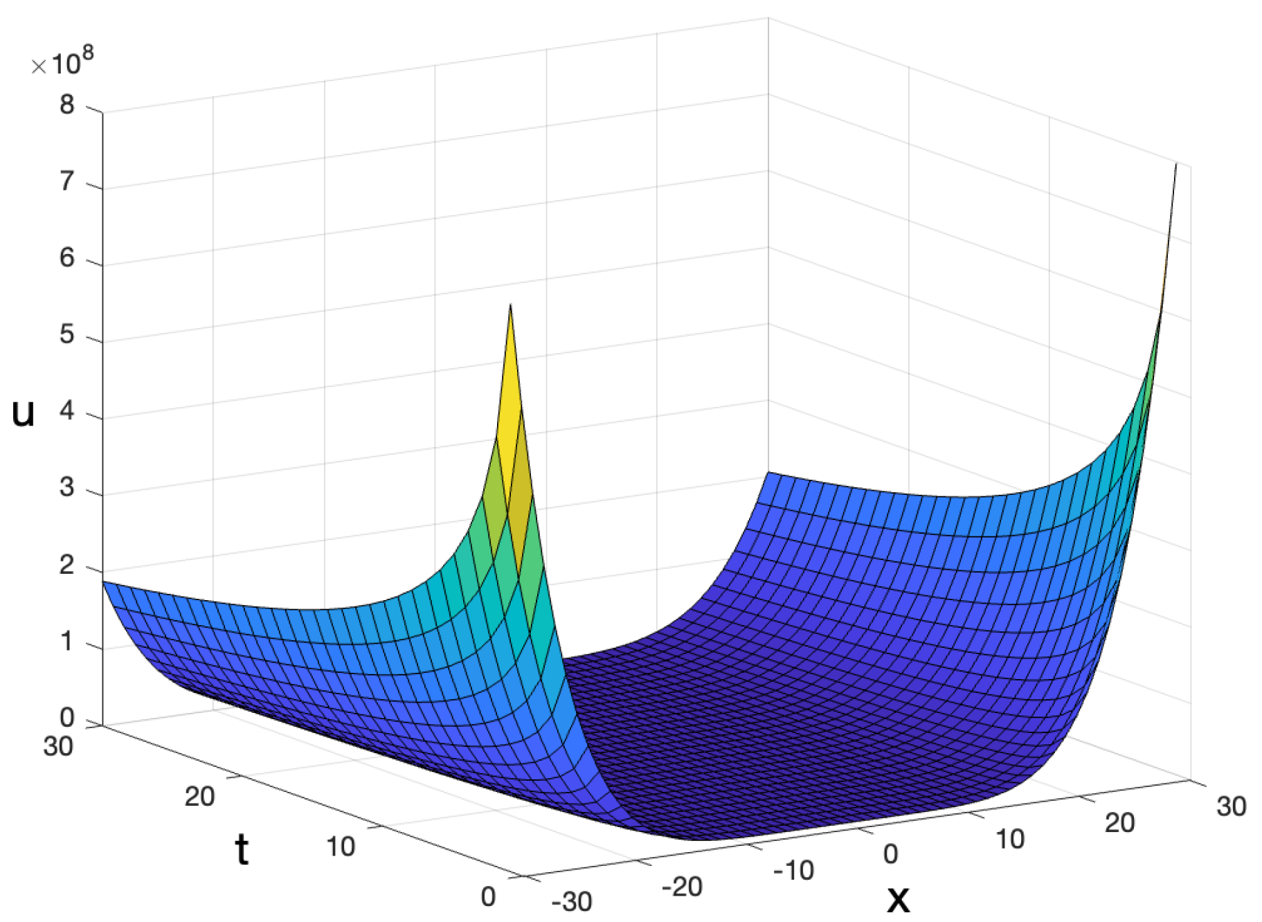
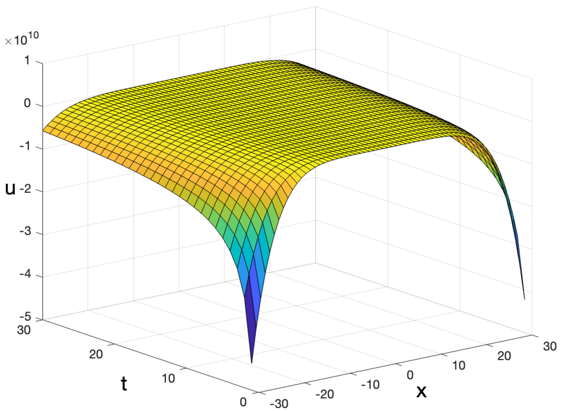
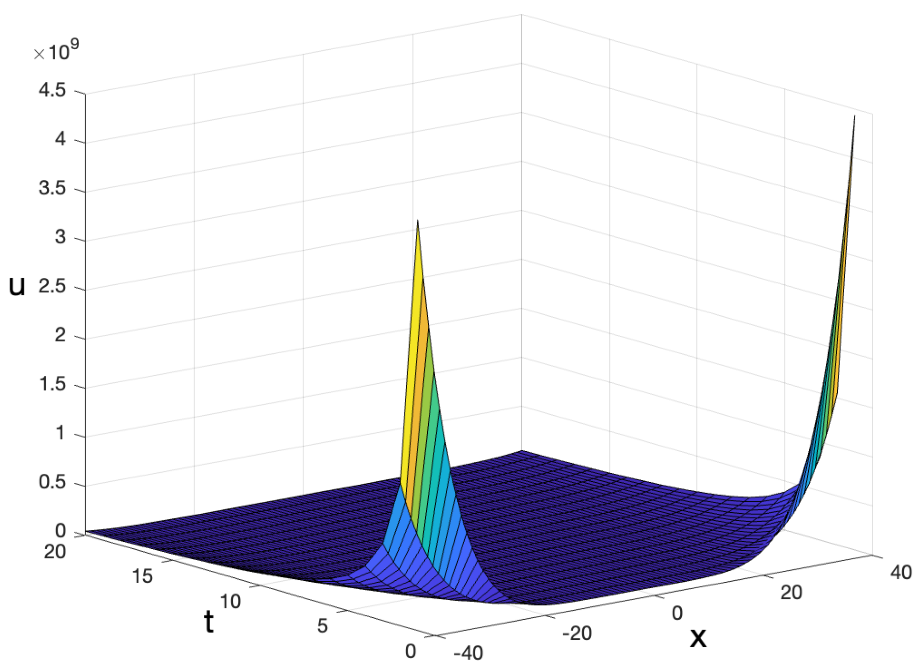
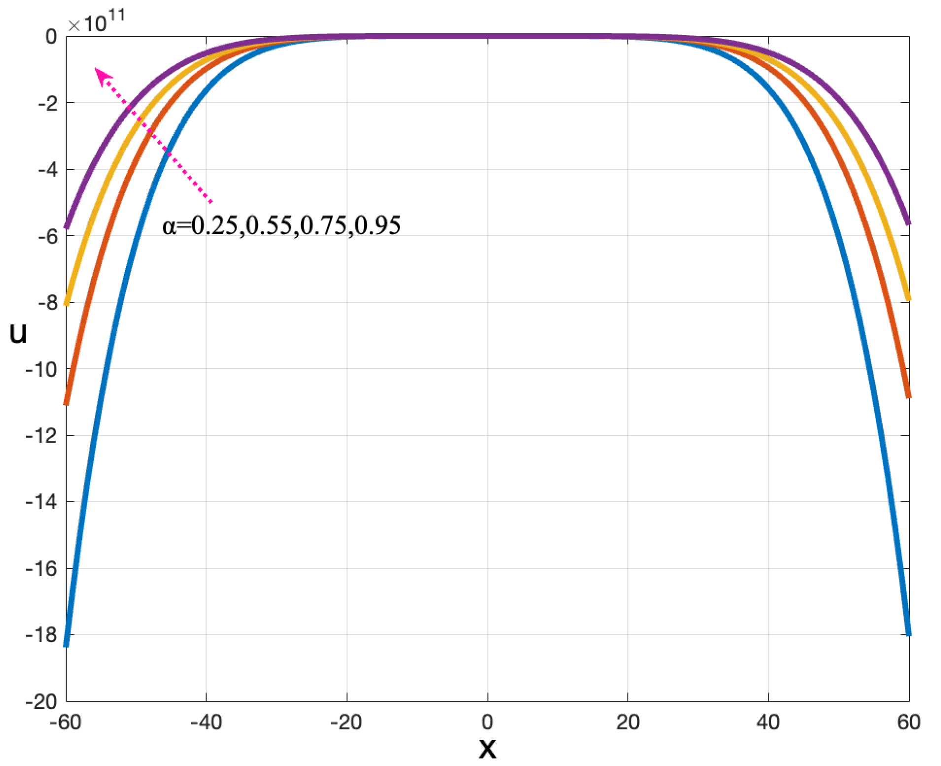
7. Graphical Illustrations of the Power Series Solutions

The following segment discusses the plots of newly discovered power series solutions generated through Matlab. The graphs of solutions are helpful in studying exact solution types with many free independent parameters. Selecting these parameters correctly enables us to observe the structure of solutions accurately and provide a more comprehensive explanation of the dynamical behavior for the time-fractional MNW system.

The power series solutions of the time-fractional MNW system are the following

$$u(t,x)=t^{\frac{-2\alpha }{5}}f\left(\xi \right)=\sum _{k=0}^{\infty }{c}_k{x}^k{t}^{-\frac{(k+2)\alpha }{5}},v(t,x)=t^{\frac{-6\alpha }{5}}g\left(\xi \right)=\sum _{k=0}^{\infty }{d}_k{x}^k{t}^{-\frac{(k+6)\alpha }{5}},$$

(63)

where $c_k$ and $d_k$ are defined by Equations (39)–(41) with arbitrary initial conditions $c_0=f\left(0\right)$, $d_0=f\left(0\right)$, $c_1=f^{\prime }\left(0\right)$, $c_2=\frac{1}{2}{f}^{″}\left(0\right)$, $c_3=\frac{1}{3!}{f}^{″\prime }\left(0\right)$, and $c_4=\frac{1}{4!}{f}^{″″}\left(0\right)$.

In the following, we use different parameter values to represent our obtained power series solutions. For a given initial condition $c_0,d_0,c_1,c_2,c_3,c_4=1$, these figures show that the fractional order difference affects the velocity $u(t,x)$ and height $v(t,x)$ variation of the free wave surface.

Figure 1 and Figure 2 show the three-dimensional images of u and v at $\alpha$ = 0.25. We observe the morphology of the free waves for the positive power series solution u and the negative power series solution v. These plots were obtained by choosing the parameters $b_1=-6$, $b_2=-2$, $b_3=96$, $b_4=160$, $a_1=1$, $a_2=-20$, $a_3=-50$, $a_4=80$, $a_5=1$, and $\alpha =0.25$.

Figure 3 and Figure 4 show the three-dimensional images of u and v at $\alpha$ = 0.95. They remain constant in the positive and negative directions. These plots are obtained by choosing parameters of $b_1=-6$, $b_2=-2$, $b_3=96$, $b_4=160$, $a_1=1$, $a_2=-20$, $a_3=-50$, $a_4=80$, $a_5=1$, and $\alpha =0.95$.

Figure 5 and Figure 6 show the two-dimensional images of u and v when $\alpha$ is taken at 0.25, 0.55, 0.75, and 0.95 for $t=2$. These images clearly show the variation of u and v for different values of $\alpha$, confirming that the wave around the cusp tends to flatten as $\alpha$ increases.

To summarize, through the observation of the three-dimensional and two-dimensional images of the wave speed $u(x,t)$ and height $v(x,t)$, it is observed that as $\alpha$ increases, the direction of the cusp and the amplitude remain unchanged and the overall solution gradually converges. This enables us to gain a better understanding of the developmental history of the obtained solution and validate the necessity of extending the integer-order equation to the time-fractional-order equation. In other words, the time-fractional MNW system is a more appropriate representation of the continuous trends observed in real-life scenarios than the classical system.

8. Conclusions

In this work, employing a Lie symmetry analysis, we established Lie symmetries for the time-fractional MNW system within the interval $0<\alpha ⩽1$ and reduced the system described in system (3) to a fractional ordinary differential system. Furthermore, we obtained power series solutions for the simplified system and verified that the exact solutions acquired through the Lie symmetry analysis exhibit a strong convergence. We generated three-dimensional and two-dimensional graphs of the respective analytical solutions to understand the physical characteristics of the power series solutions and the influence of the fractional order $\alpha$ on said solutions. These graphs illustrate the dynamical evolution at different values of $\alpha$. Another significant achievement is presenting the conservation laws for each of the Lie symmetries of the model through Ibragimov’s new conservation law theorem.

References

1. Clarkson, P.A.; Dowie, E. Rational solutions of the Boussinesq equation and applications to rogue waves. Trans. Math. Its Appl. 2017, 1, tnx003. [Google Scholar] [CrossRef] [Green Version]
2. Akbar, M.A.; Akinyemi, L.; Yao, S.W.; Jhangeer, A.; Rezazadeh, H.; Khater, M.M.; Ahmad, H.; Inc, M. Soliton solutions to the Boussinesq equation through sine-Gordon method and Kudryashov method. Results Phys. 2021, 25, 104228. [Google Scholar] [CrossRef]
3. Mikhailov, A.V.; Novikov, V.S.; Wang, J.P. On classification of integrable nonevolutionary equations. Stud. Appl. Math. 2007, 118, 419–457. [Google Scholar] [CrossRef] [Green Version]
4. Akbulut, A.; Kaplan, M.; Kaabar, M.K. New exact solutions of the Mikhailov-Novikov-Wang equation via three novel techniques. J. Ocean Eng. Sci. 2021, 8, 103–110. [Google Scholar] [CrossRef]
5. Raza, N.; Seadawy, A.R.; Arshed, S.; Rafiq, M.H. A variety of soliton solutions for the Mikhailov-Novikov-Wang dynamical equation via three analytical methods. J. Geom. Phys. 2022, 176, 104515. [Google Scholar] [CrossRef]
6. Ray, S.S.; Singh, S. New various multisoliton kink-type solutions of the (1+ 1)-dimensional Mikhailov–Novikov–Wang equation. Math. Methods Appl. Sci. 2021, 44, 14690–14702. [Google Scholar]
7. Ray, S.S. Painlevé analysis, group invariant analysis, similarity reduction, exact solutions, and conservation laws of Mikhailov–Novikov–Wang equation. Int. J. Geom. Methods Mod. Phys. 2021, 18, 2150094. [Google Scholar] [CrossRef]
8. Demiray, S.T.; Bayrakci, U. A study on the solutions of (1+ 1)-dimensional mikhailov-novikov-wang equation. Math. Model. Numer. Simul. Appl. 2022, 2, 1–8. [Google Scholar] [CrossRef]
9. Sergyeyev, A. Zero curvature representation for a new fifth-order integrable system. arXiv 2006, arXiv:nlin/0604064. [Google Scholar] [CrossRef] [Green Version]
10. Sierra, C.A.G. A new travelling wave solution of the Mikhail-Novikov-Wang system usint the extended tanh method. Bol. Mat. 2007, 14, 38–43. [Google Scholar]
11. Carreno, J.C.L.; Suáres, R.M. Acerca de algunas soluciones de ciertas ecuaciones de onda. Bol. Mat. 2012, 19, 107–118. [Google Scholar]
12. Shan, X.; Zhu, J. The Mikhauilov-Novikov-Wang hierarchy and its Hamiltonian structures. Acta Phys. Pol.-Ser. B Elem. Part. Phys. 2012, 43, 1953. [Google Scholar] [CrossRef]
13. Singh, J.; Kumar, D.; Kılıçman, A. Numerical solutions of nonlinear fractional partial differential equations arising in spatial diffusion of biological populations. Abstr. Appl. Anal. 2014, 2014, 535793. [Google Scholar] [CrossRef] [Green Version]
14. Liaskos, K.B.; Pantelous, A.A.; Kougioumtzoglou, I.A.; Meimaris, A.T.; Pirrotta, A. Implicit analytic solutions for a nonlinear fractional partial differential beam equation. Commun. Nonlinear Sci. Numer. Simul. 2020, 85, 105219. [Google Scholar] [CrossRef]
15. Liu, H.Z.; Wang, Z.G.; Xin, X.P.; Liu, X.Q. Symmetries, symmetry reductions and exact solutions to the generalized nonlinear fractional wave equations. Commun. Theor. Phys. 2018, 70, 014. [Google Scholar] [CrossRef]
16. Hashemi, M.S.; Baleanu, D. Lie Symmetry Analysis of Fractional Differential Equations; CRC Press: Boca Raton, FL, USA, 2020. [Google Scholar]
17. Zhang, Y. A finite difference method for fractional partial differential equation. Appl. Math. Comput. 2009, 215, 524–529. [Google Scholar] [CrossRef]
18. Li, C.; Zeng, F. Finite difference methods for fractional differential equations. Int. J. Bifurc. Chaos 2012, 22, 1230014. [Google Scholar] [CrossRef]
19. Odibat, Z. On the optimal selection of the linear operator and the initial approximation in the application of the homotopy analysis method to nonlinear fractional differential equations. Appl. Numer. Math. 2019, 137, 203–212. [Google Scholar] [CrossRef]
20. Karaagac, B. New exact solutions for some fractional order differential equations via improved sub-equation method. Discret. Contin. Dyn. Syst. 2019, 12, 447–454. [Google Scholar] [CrossRef] [Green Version]
21. Kadkhoda, N.; Jafari, H. Application of fractional sub-equation method to the space-time fractional differential equations. Int. J. Adv. Appl. Math. Mech. 2017, 4, 1–6. [Google Scholar]
22. Cheng, X.; Wang, L.; Hou, J. Solving time fractional Keller–Segel type diffusion equations with symmetry analysis, power series method, invariant subspace method and q-homotopy analysis method. Chin. J. Phys. 2022, 77, 1639–1653. [Google Scholar] [CrossRef]
23. Maheswari, C.U.; Bakshi, S.K. Invariant subspace method for time-fractional nonlinear evolution equations of the third order. Pramana 2022, 96, 173. [Google Scholar] [CrossRef]
24. Prakash, P.; Thomas, R.; Bakkyaraj, T. Invariant subspaces and exact solutions: (1 + 1) and (2 + 1)-dimensional generalized time-fractional thin-film equations. Comput. Appl. Math. 2023, 42, 97. [Google Scholar] [CrossRef]
25. Arqub, O.A.; Hayat, T.; Alhodaly, M. Analysis of lie symmetry, explicit series solutions, and conservation laws for the nonlinear time-fractional phi-four equation in two-dimensional space. Int. J. Appl. Comput. Math. 2022, 8, 145. [Google Scholar] [CrossRef]
26. Al-Deiakeh, R.; Arqub, O.A.; Al-Smadi, M.; Momani, S. Lie symmetry analysis, explicit solutions, and conservation laws of the time-fractional Fisher equation in two-dimensional space. J. Ocean Eng. Sci. 2022, 7, 345–352. [Google Scholar] [CrossRef]
27. Yu, J.; Feng, Y.; Wang, X. Lie symmetry analysis and exact solutions of time fractional Black–Scholes equation. Int. J. Financ. Eng. 2022, 9, 2250023. [Google Scholar] [CrossRef]
28. Zhang, Z.Y.; Zhu, H.M.; Zheng, J. Lie symmetry analysis, power series solutions and conservation laws of the time-fractional breaking soliton equation. Waves Random Complex Media 2022, 32, 3032–3052. [Google Scholar] [CrossRef]
29. Tian, S.F. Lie symmetry analysis, conservation laws and solitary wave solutions to a fourth-order nonlinear generalized Boussinesq water wave equation. Appl. Math. Lett. 2020, 100, 106056. [Google Scholar] [CrossRef]
30. Olver, P.J. Applications of Lie Groups to Differential Equations; Springer Science & Business Media: Berlin/Heidelberg, Germany, 1993; Volume 107. [Google Scholar]
31. Gazizov, R.; Kasatkin, A.; Lukashchuk, S.Y. Continuous transformation groups of fractional differential equations. Vestn. Usatu 2007, 9, 21. [Google Scholar]
32. Gazizov, R.; Kasatkin, A.; Lukashchuk, S.Y. Symmetry properties of fractional diffusion equations. Phys. Scr. 2009, 2009, 014016. [Google Scholar] [CrossRef]
33. Zhang, Z.Y. Symmetry determination and nonlinearization of a nonlinear time-fractional partial differential equation. Proc. R. Soc. A 2020, 476, 20190564. [Google Scholar] [CrossRef] [Green Version]
34. Jefferson, G.; Carminati, J. FracSym: Automated symbolic computation of Lie symmetries of fractional differential equations. Comput. Phys. Commun. 2014, 185, 430–441. [Google Scholar] [CrossRef]
35. Angstmann, C.N.; Henry, B.I. Generalized fractional power series solutions for fractional differential equations. Appl. Math. Lett. 2020, 102, 106107. [Google Scholar] [CrossRef]
36. Ibragimov, N.H. Nonlinear self-adjointness and conservation laws. J. Phys. A Math. Theor. 2011, 44, 432002. [Google Scholar] [CrossRef]
37. Ibragimov, N.H. A new conservation theorem. J. Math. Anal. Appl. 2007, 333, 311–328. [Google Scholar] [CrossRef] [Green Version]
Figure 1. Three-dimensional graphs of u ( x , t ) for α = 0.25 .
Fractalfract 07 00457 g001
Figure 2. Three-dimensional graphs of v ( x , t ) for α = 0.25 .
Fractalfract 07 00457 g002
Figure 3. Three-dimensional graphs of u ( x , t ) for α = 0.95 .
Fractalfract 07 00457 g003
Figure 4. Three-dimensional graphs of v ( x , t ) for α = 0.95 .
Fractalfract 07 00457 g004
Figure 5. Two-dimensional graphs of u ( x , t ) for t = 2 .
Fractalfract 07 00457 g005
Figure 6. Two-dimensional graphs of v ( x , t ) for t = 2 .
Fractalfract 07 00457 g006
Disclaimer/Publisher’s Note: The statements, opinions and data contained in all publications are solely those of the individual author(s) and contributor(s) and not of MDPI and/or the editor(s). MDPI and/or the editor(s) disclaim responsibility for any injury to people or property resulting from any ideas, methods, instructions or products referred to in the content.