
A Fractional-Order Total Variation Regularization-Based Method for Recovering Geiger-Mode Avalanche Photodiode Light Detection and Ranging Depth Images

 , , and
Abstract
:1. Introduction
2. FOTV Regularization Recovery Model
2.1. TV Regularization Recovery Model
2.2. TV-Regularization Recovery Model
2.3. FOTV-Regularization Recovery Model
2.4. Solution of the FOTV-Regularization Recovery Model
| Algorithm 1: Split Bregman Algorithm for Solving Recovery Models for Anisotropic FOTV Regularization |
| Initialization: While End while |
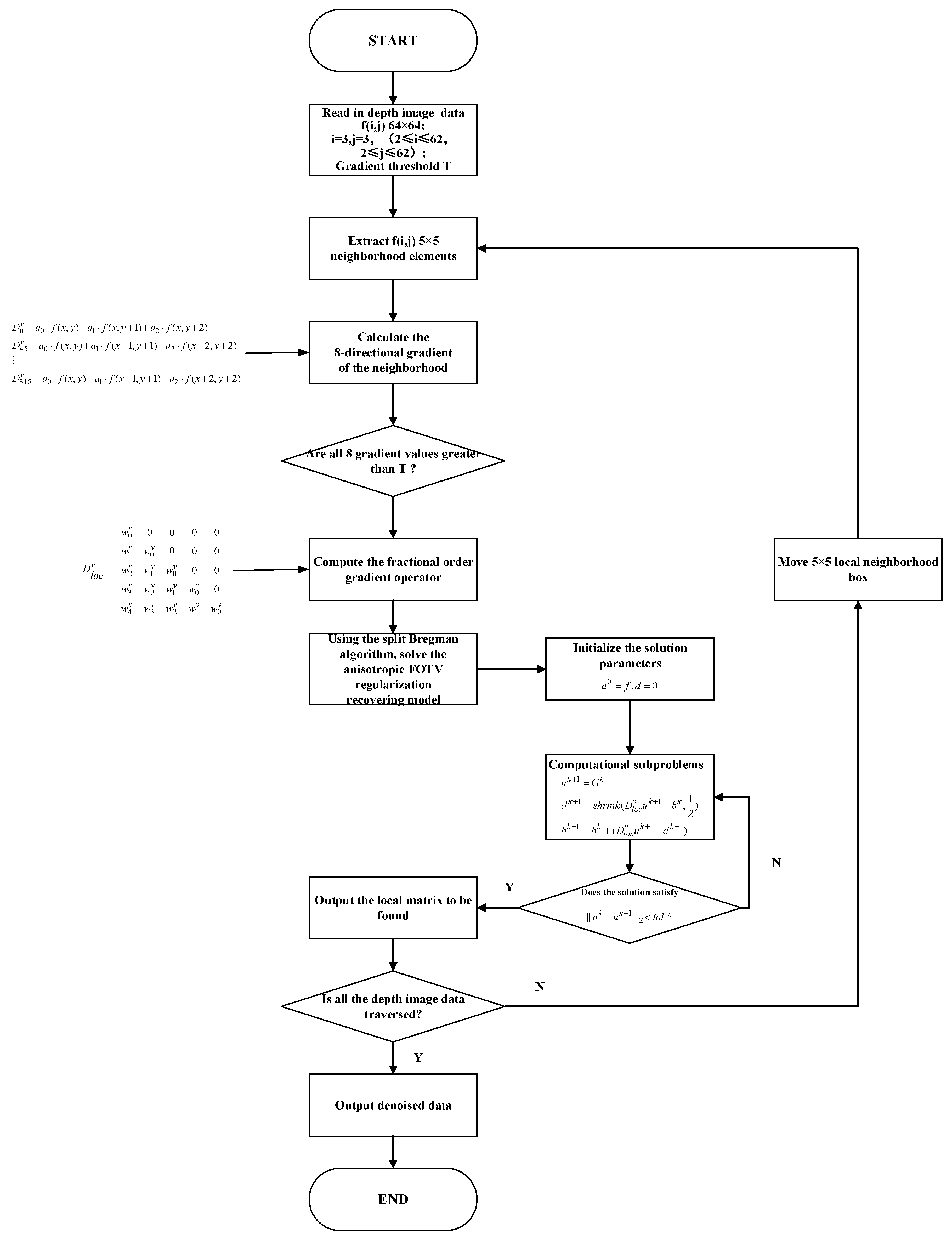
3. GM-APD Depth Image FOTV Restoration Algorithm
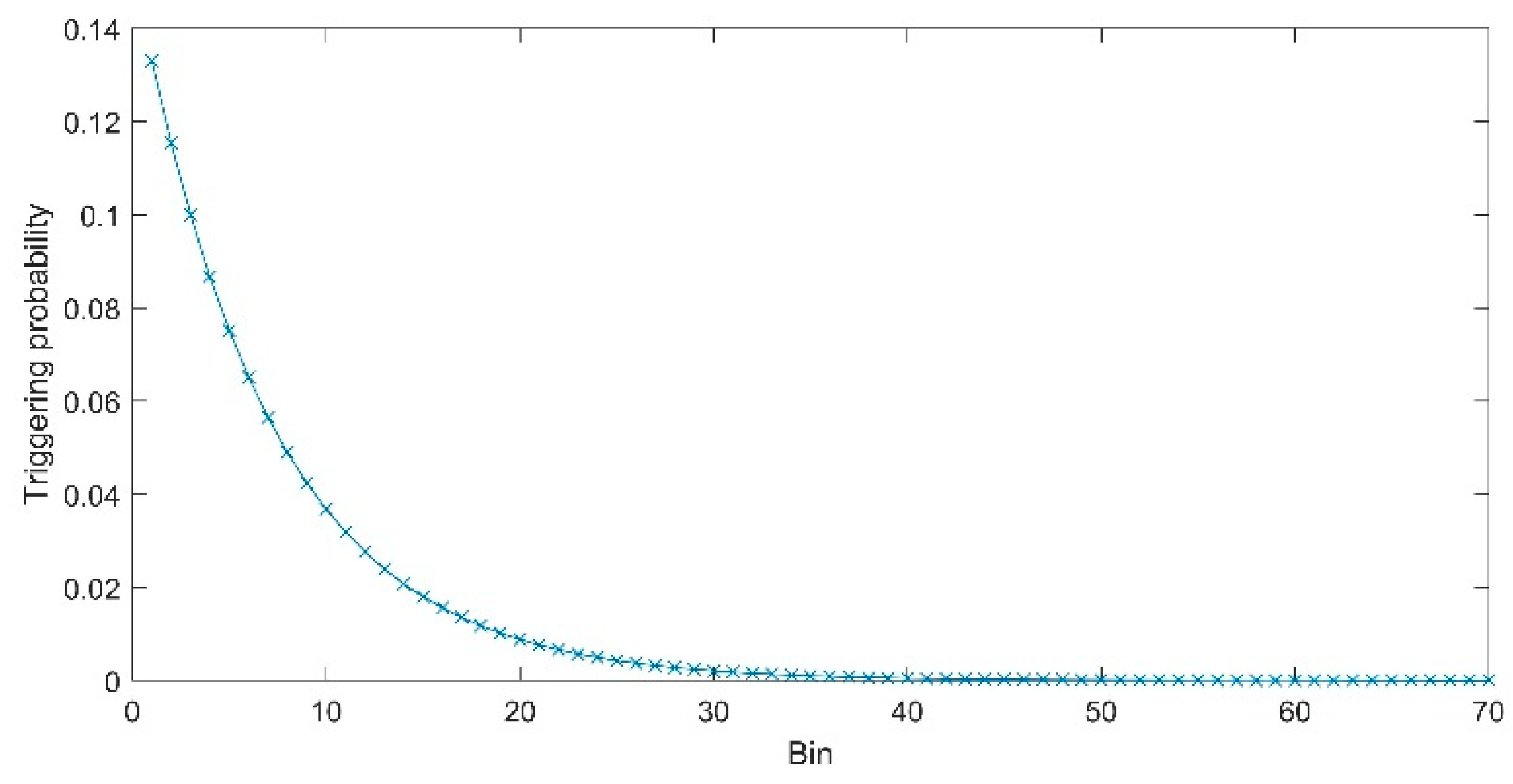
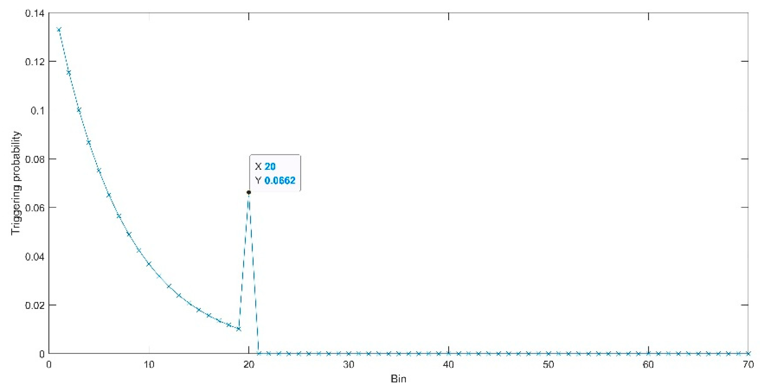
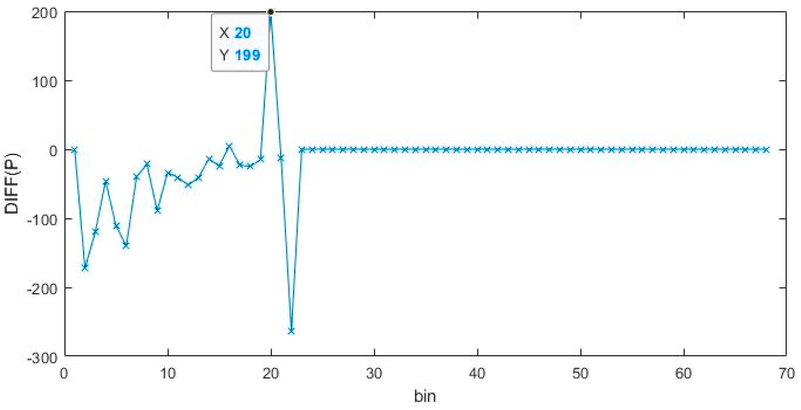
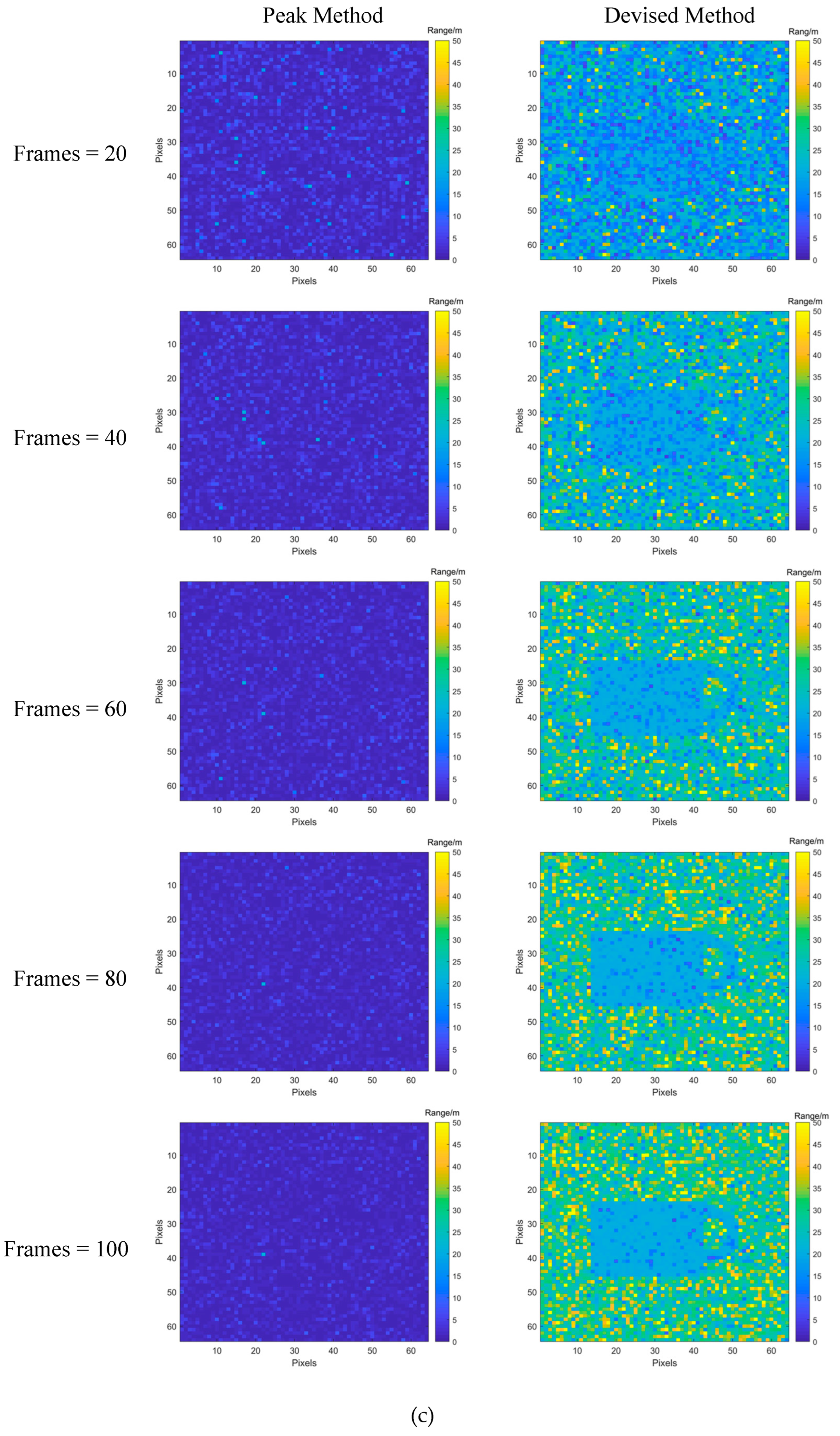
3.1. Depth-Image Extraction from Low SBR and Few-Frame Data Using a Spatial-Domain Differential Peak-Picking Method
3.2. FOTV-Regularization Recovery Algorithm
4. Simulation and Experimental Verification
4.1. Evaluation Metrics
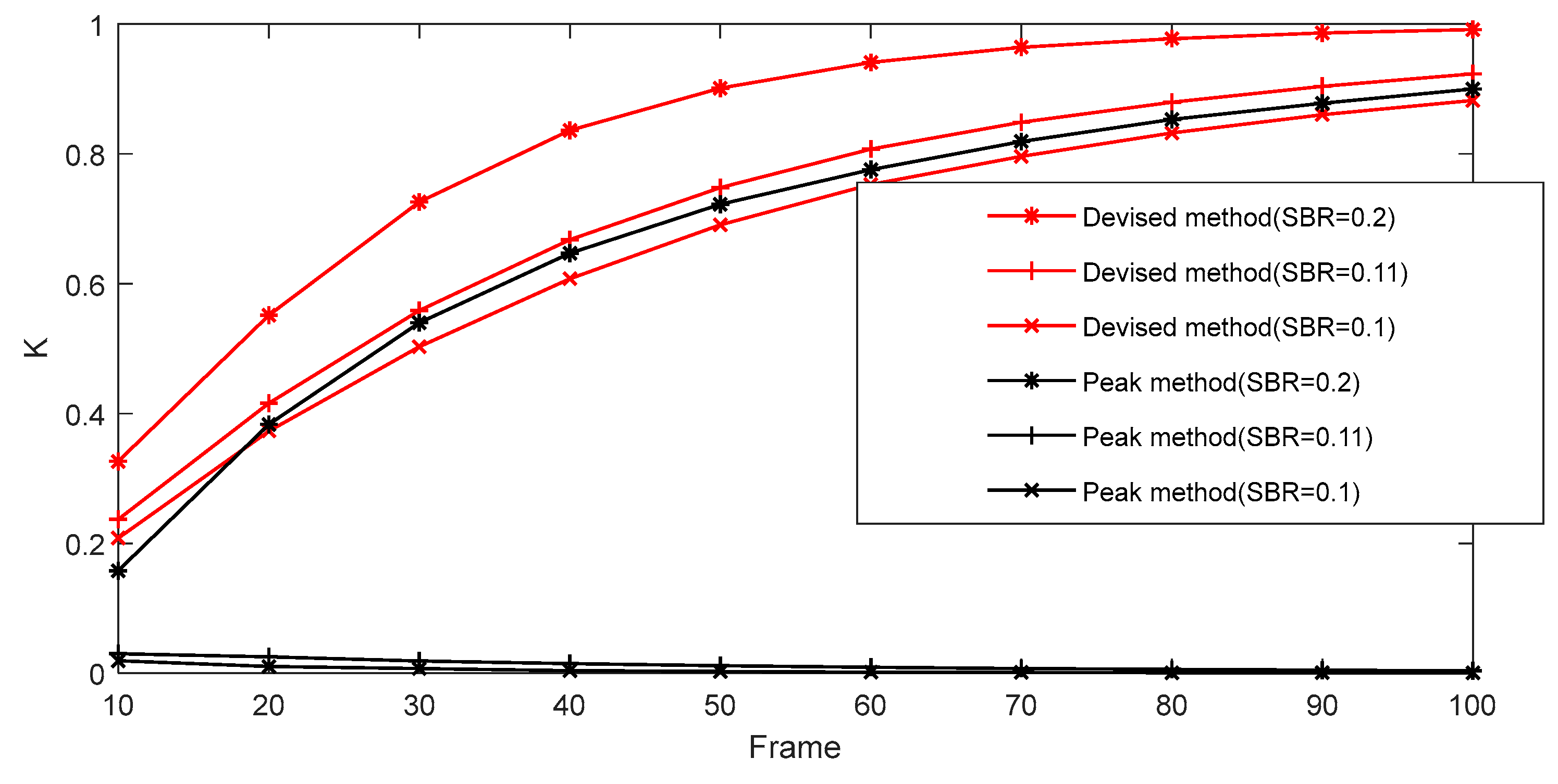
4.1.1. K
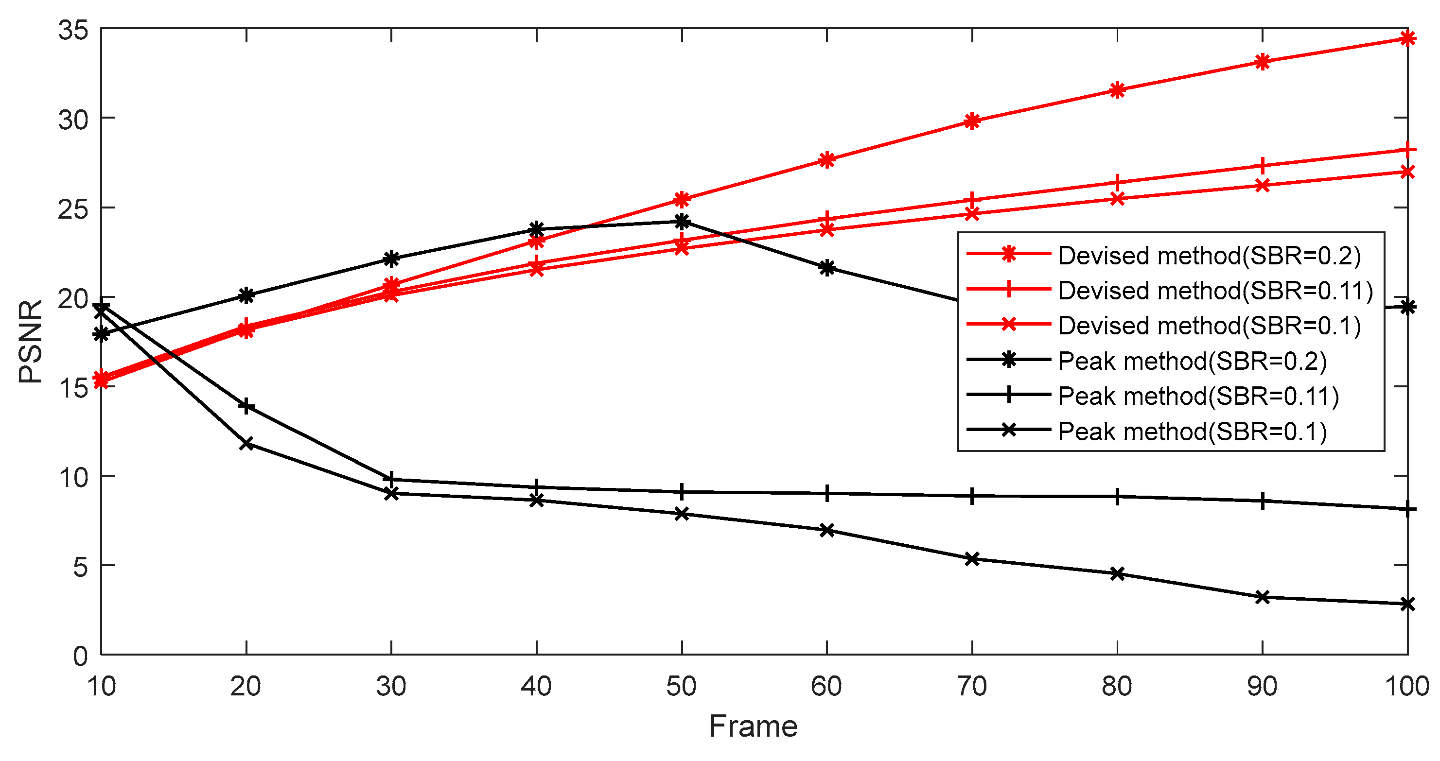
4.1.2. PSNR
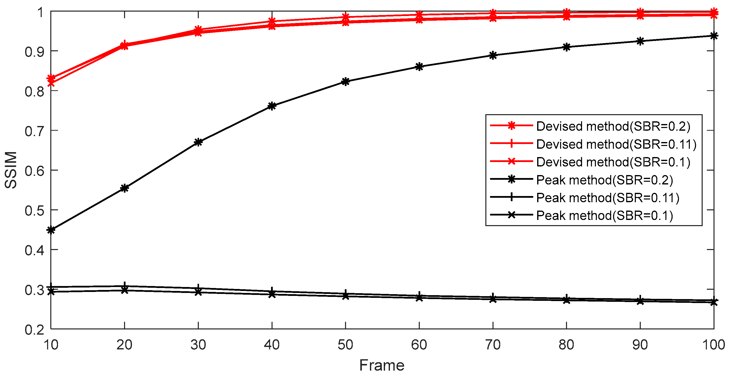
4.1.3. SSIM
4.2. Simulation Analysis
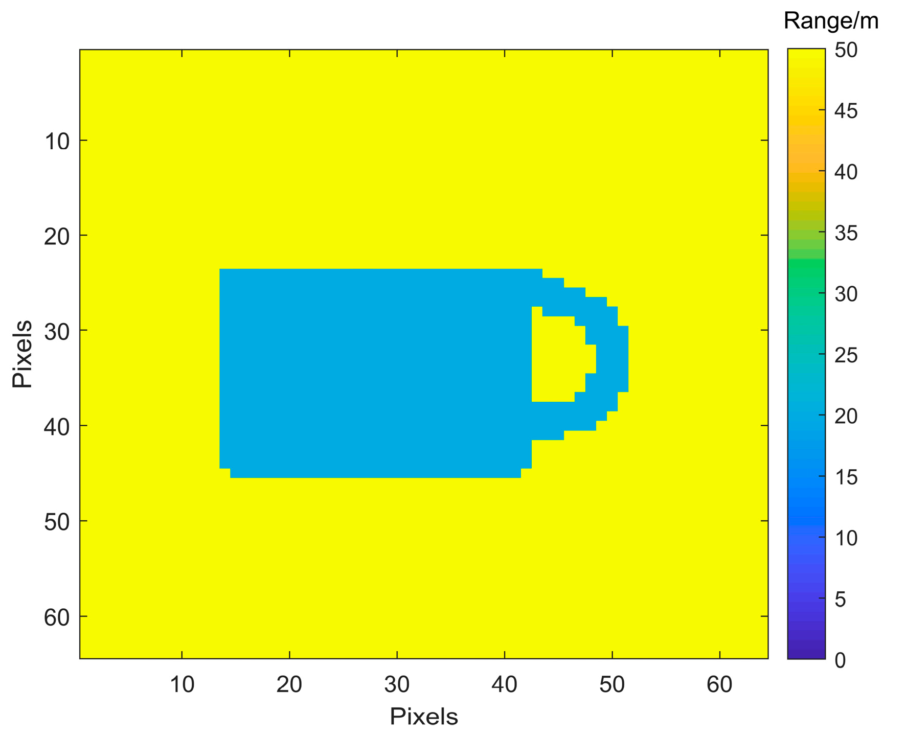
4.2.1. Depth Image Extraction
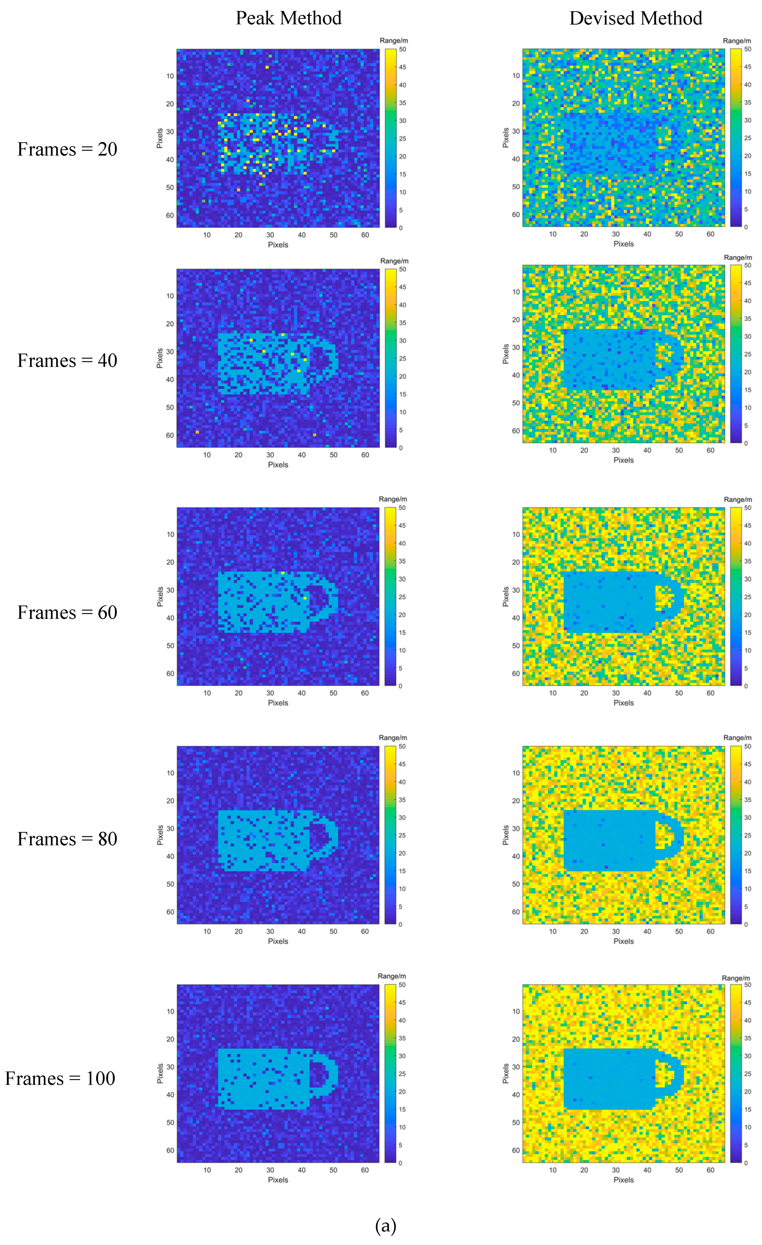
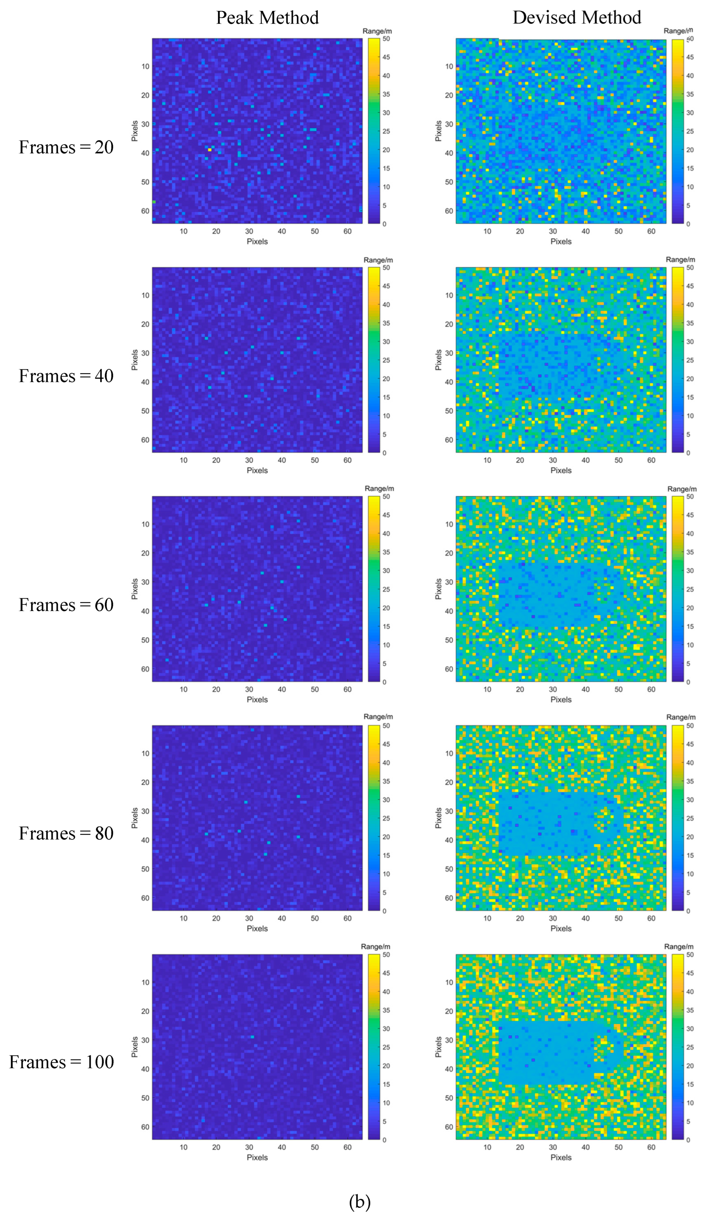
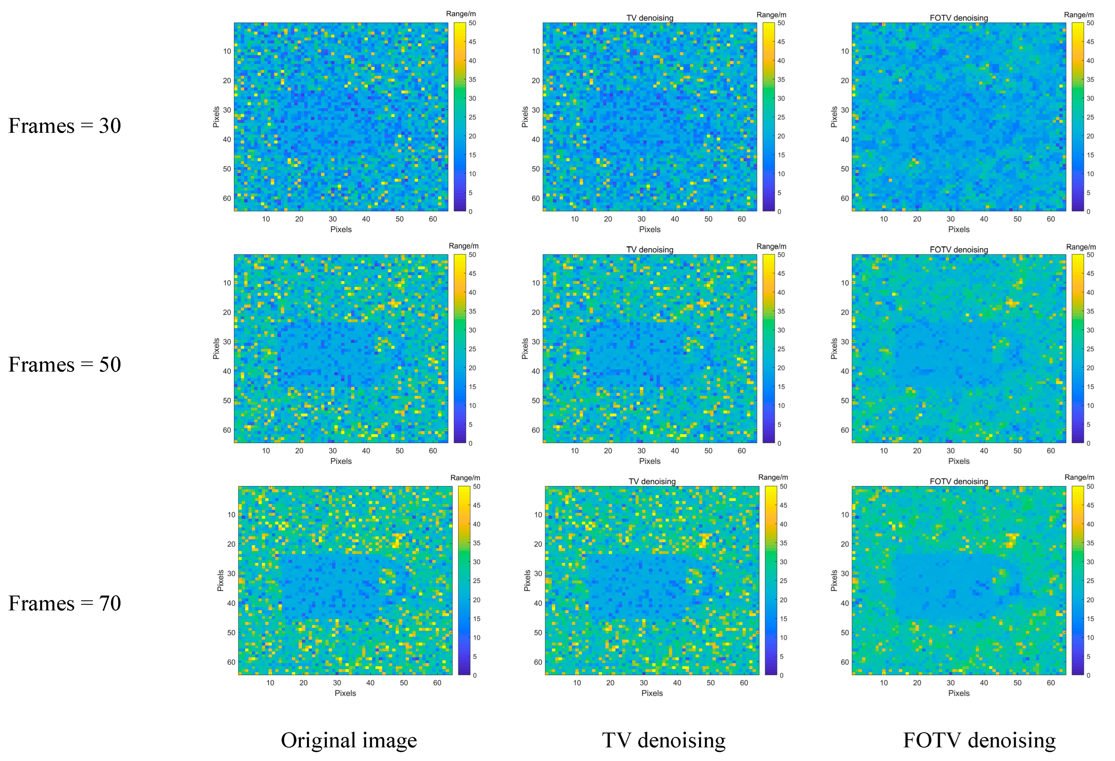
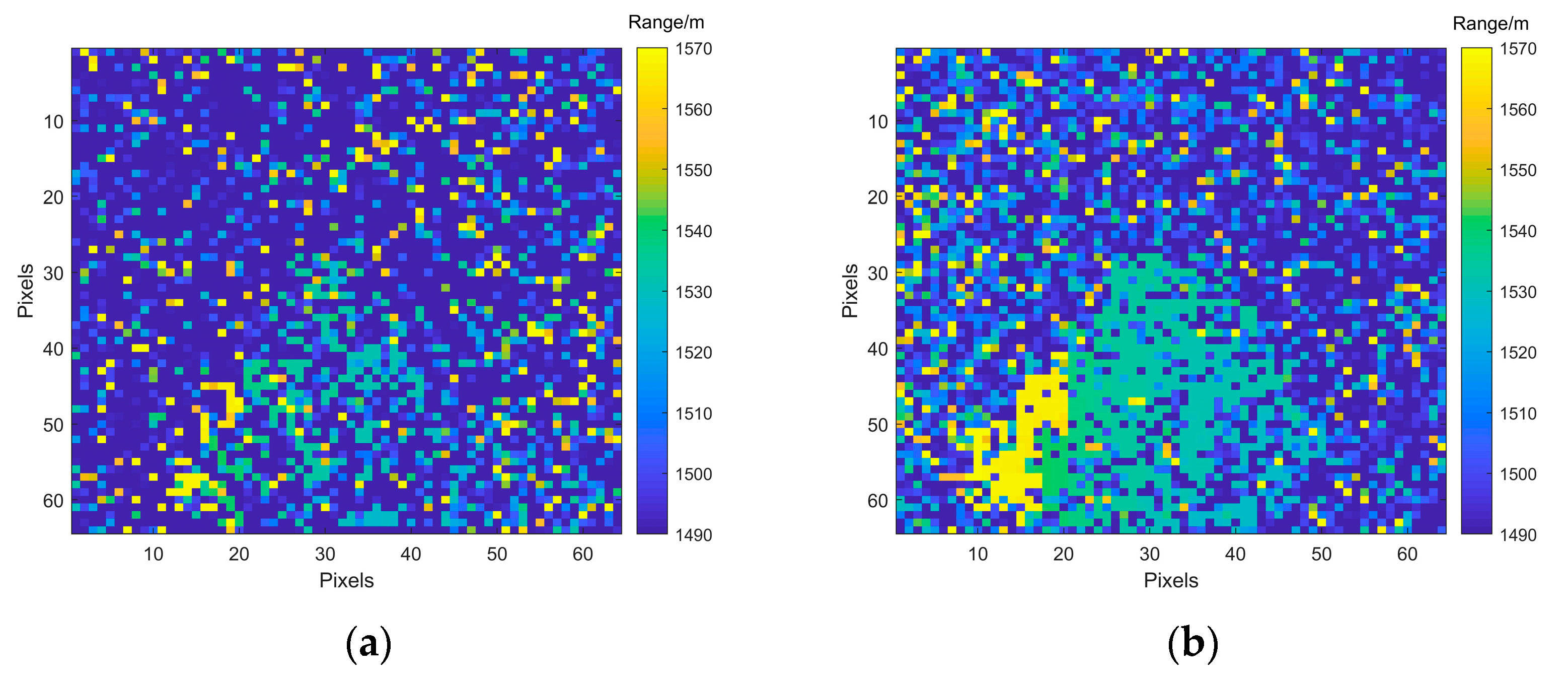
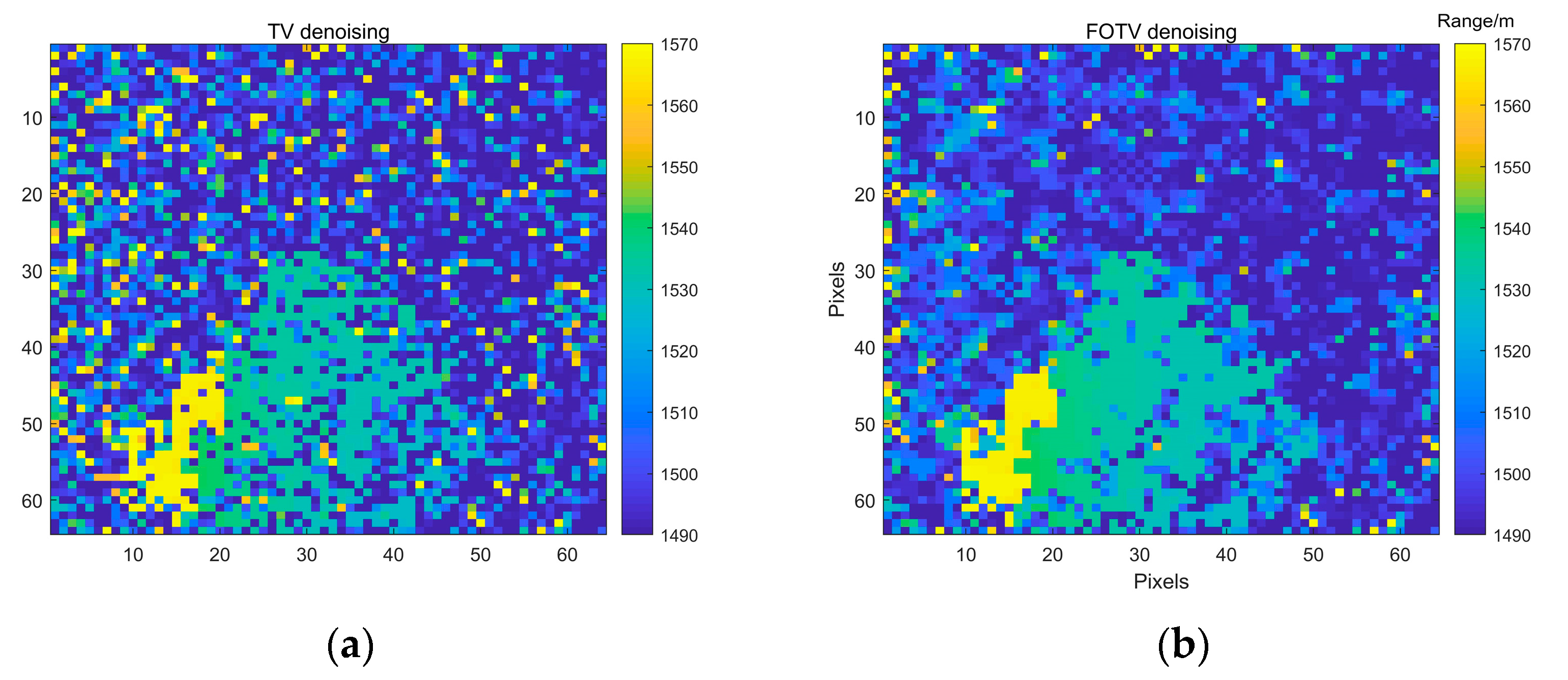
4.2.2. Depth-Image Recovery Using the FOTV Method
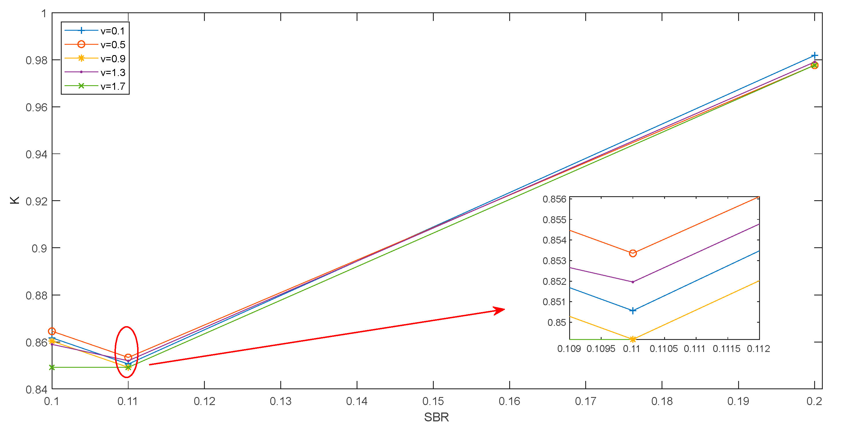
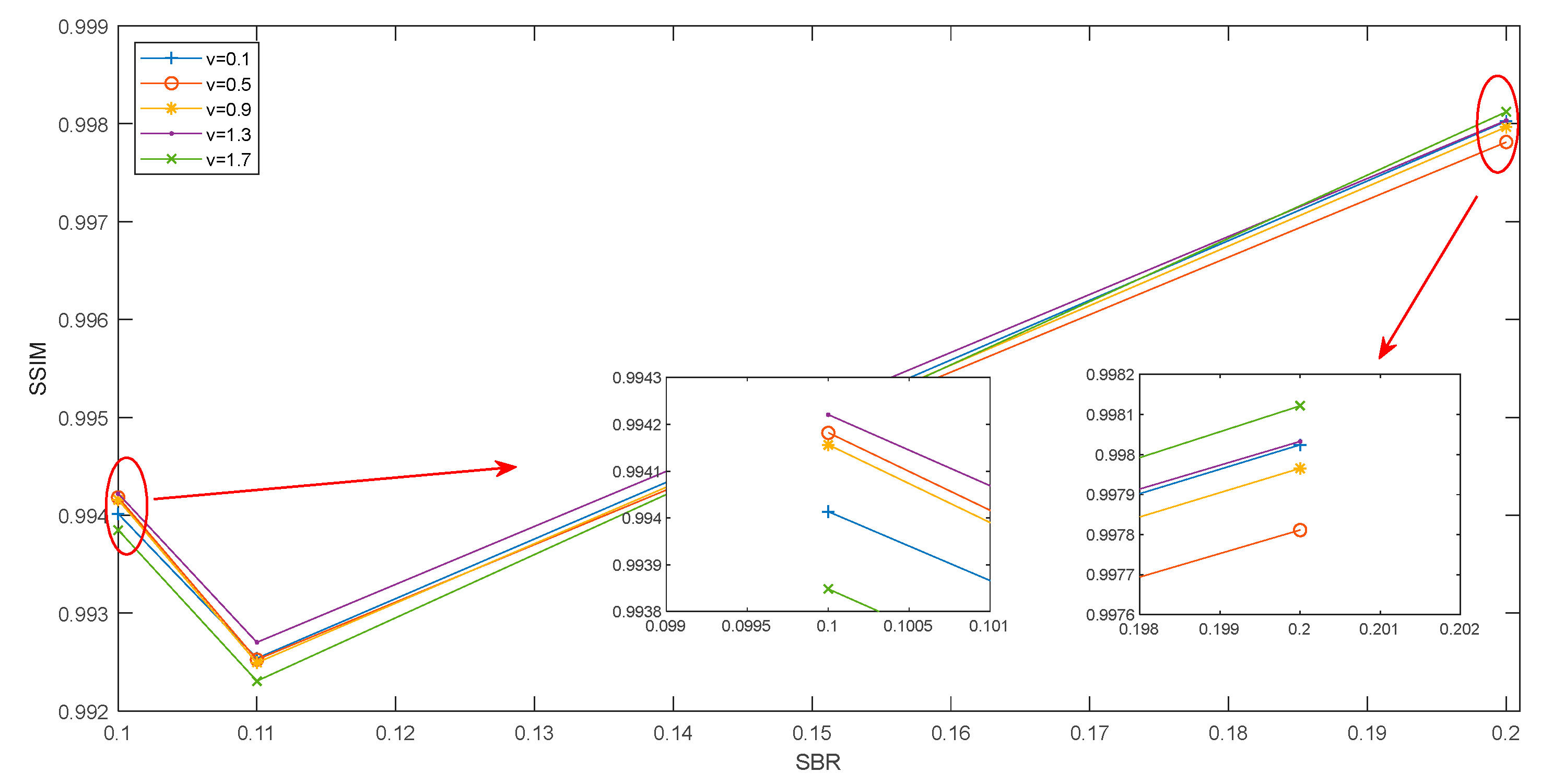
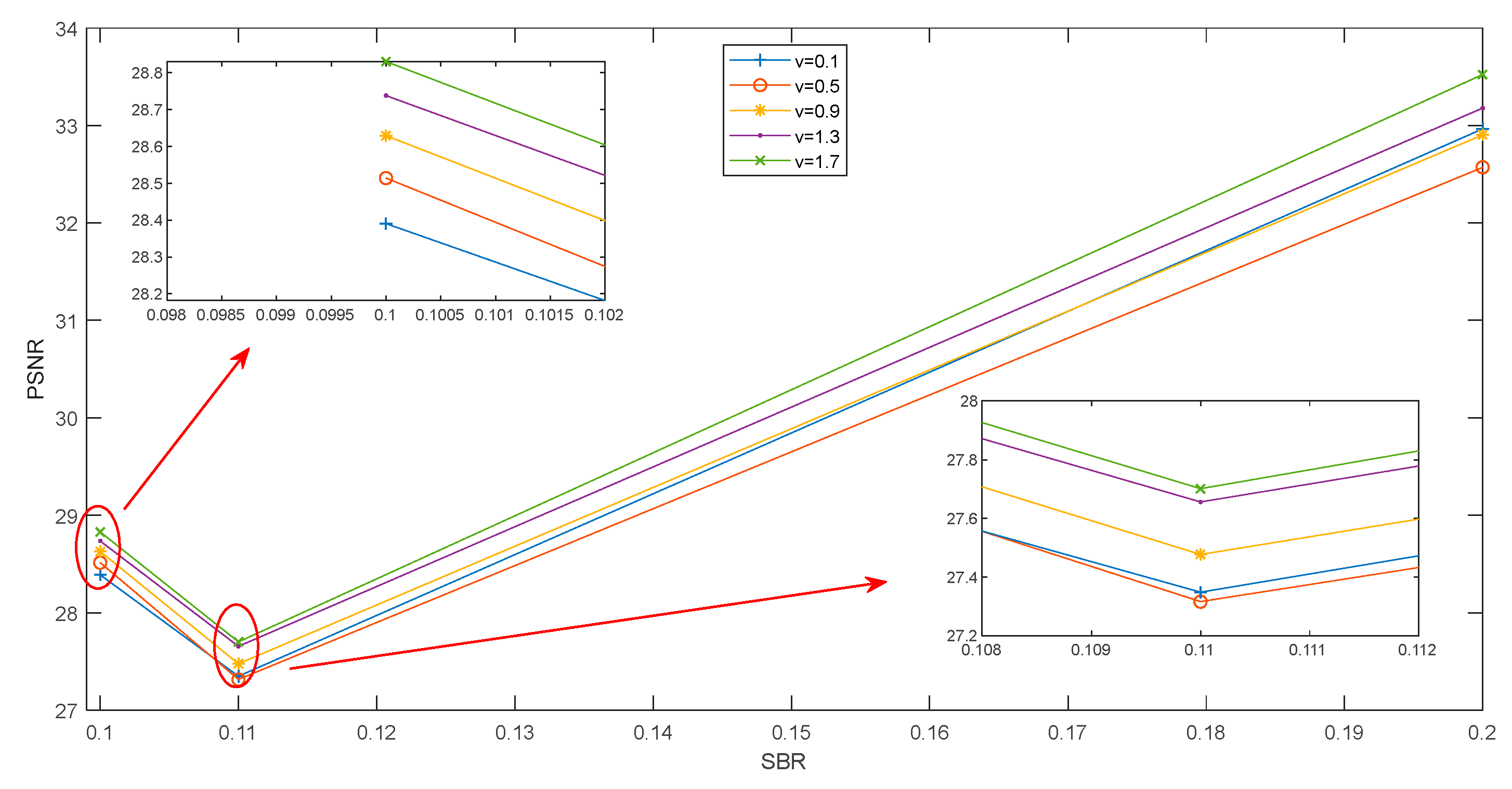
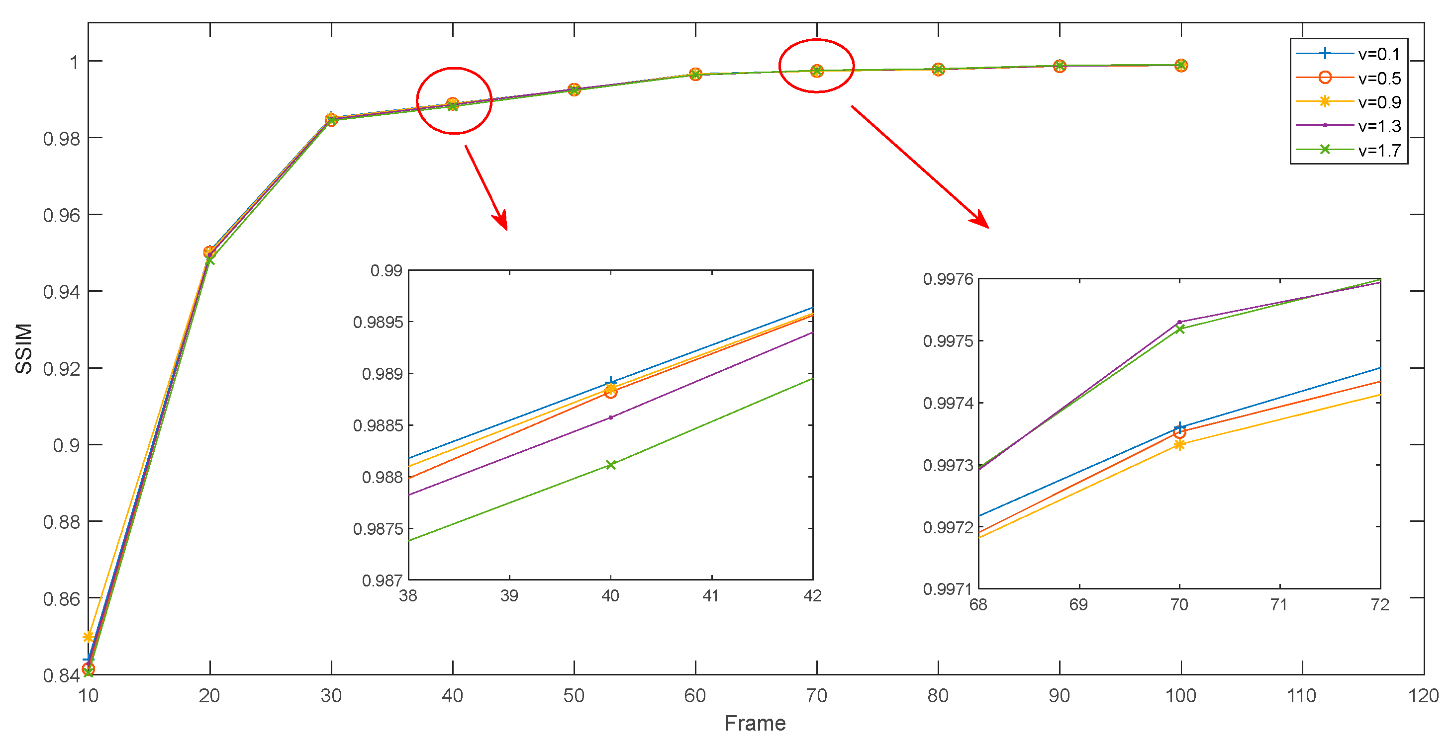
- Selection of optimal fractional order for fractional calculus
- 2.
- FOTV-recovery algorithm
4.3. Experimental Verification
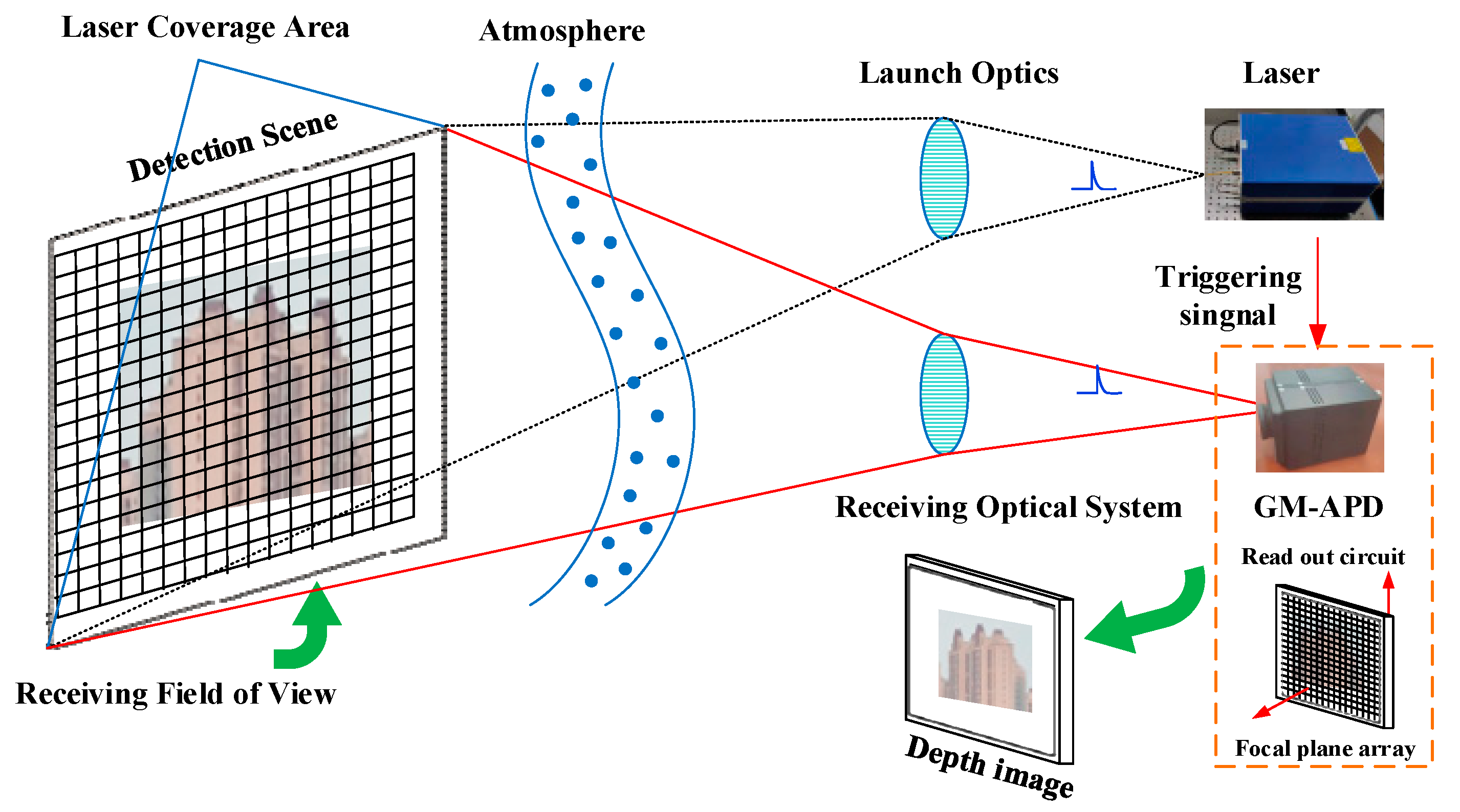
4.3.1. Experimental Platform
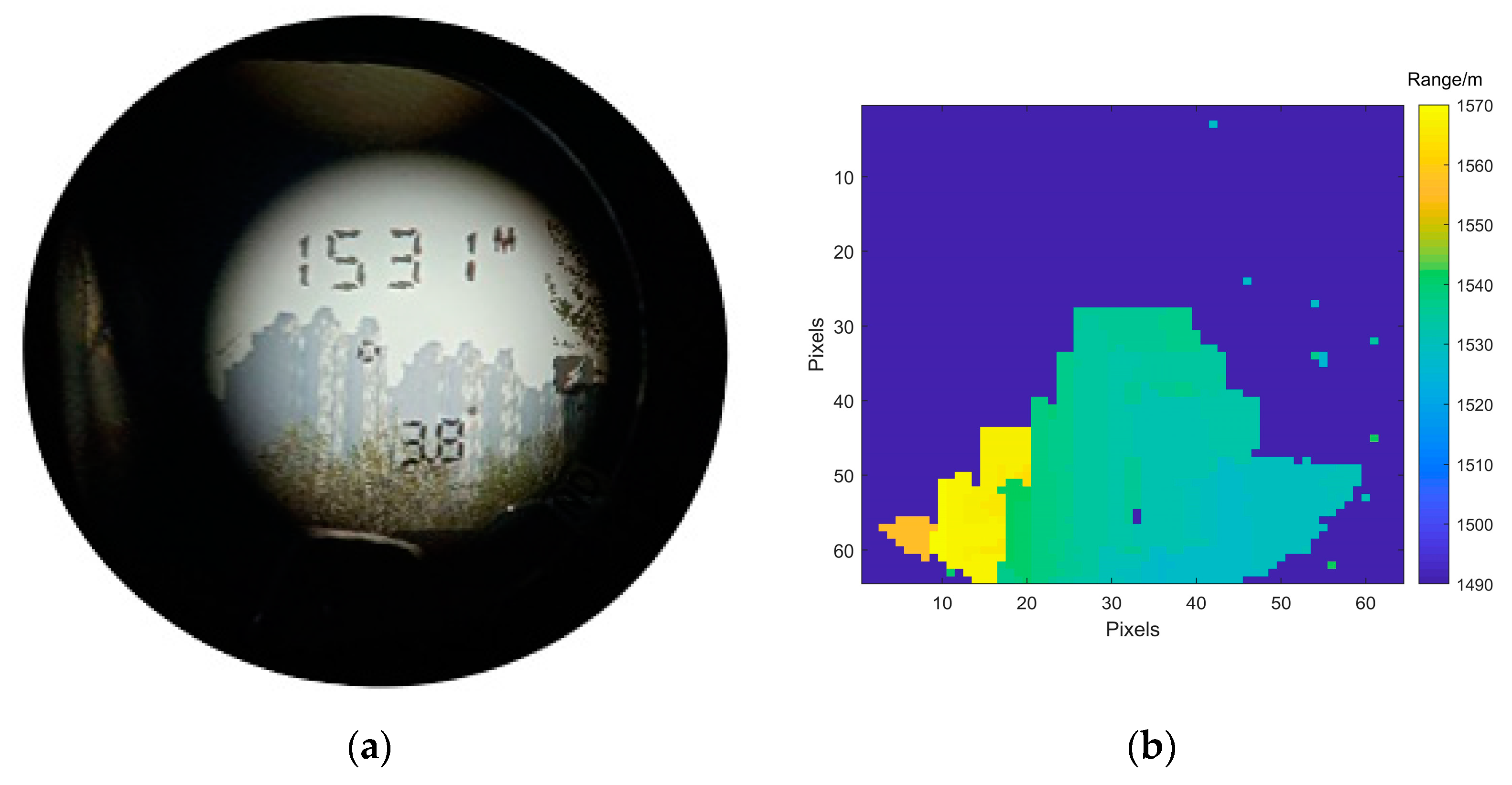
4.3.2. Outdoor Experiment
5. Discussion
Author Contributions
Funding
Data Availability Statement
Conflicts of Interest
References
- Shi, X.; Lu, W.; Sun, J.; Ge, W.; Zhang, H.; Li, S. Suppressing the influence of GM-APD coherent lidar saturation by signal modulation. Optik 2023, 275, 170619. [Google Scholar] [CrossRef]
- Ding, Y.; Qu, Y.; Sun, J.; Du, D.; Jiang, Y.; Zhang, H. Long-distance multi-vehicle detection at night based on Gm-APD lidar. Remote Sens. 2022, 14, 3553. [Google Scholar] [CrossRef]
- Dai, J.; Li, S.; Gao, F.; Cao, H.; Guo, G.; Liu, X.; Wang, Q. Performance analysis of the photon-counting lidar based on the statistical property. In Signal and Information Processing, Networking and Computers; Sun, J., Wang, Y., Huo, M., Xu, L., Eds.; Lecture Notes in Electrical Engineering; Springer: Singapore, 2023; p. 917. [Google Scholar] [CrossRef]
- Li, Y.; Zhou, J.; Huang, F.; Liu, L. Sub-pixel extraction of laser stripe center using an improved gray-gravity method. Sensors 2017, 17, 814. [Google Scholar] [CrossRef] [PubMed]
- Liu, D.; Sun, J.; Lu, W.; Li, S.; Zhou, X. 3D reconstruction of the dynamic scene with high-speed targets for GM-APD lidar. Opt. Laser Technol. 2023, 161, 109114. [Google Scholar] [CrossRef]
- Zhang, Y.; Li, S.; Sun, J.; Liu, D.; Zhang, X.; Yang, X.; Zhou, X. Dual-parameter estimation algorithm for Gm-APD lidar depth imaging through smoke. Measurement 2022, 196, 111269. [Google Scholar] [CrossRef]
- Liu, D.; Sun, J.; Gao, S.; Ma, L.; Jiang, P.; Guo, S.; Zhou, X. Single-parameter estimation construction algorithm for Gm-APD lidar imaging through fog. Opt. Commun. 2021, 482, 126558. [Google Scholar] [CrossRef]
- Wang, M.; Sun, J.; Li, S.; Lu, W.; Zhou, X.; Zhang, H. A photon-number-based systematic algorithm for range image recovery of GM-APD lidar under few-frames detection. Infrared Phys. Technol. 2022, 125, 104267. [Google Scholar] [CrossRef]
- Zhang, Y.; Liu, Z.; Huang, M.; Zhu, Q.; Yang, B. Multi-resolution depth image restoration. Mach. Vis. Appl. 2021, 32, 65. [Google Scholar] [CrossRef]
- Kang, Y.; Xue, R.; Wang, X.; Zhang, T.; Meng, F.; Li, L.; Zhao, W. High-resolution depth imaging with a small-scale SPAD array based on the temporal-spatial filter and intensity image guidance. Opt. Express 2022, 30, 33994–34011. [Google Scholar] [CrossRef]
- Ibrahim, M.M.; Liu, Q. Optimized Color-guided Filter for Depth Image Denoising. In Proceedings of the ICASSP 2019—2019 IEEE International Conference on Acoustics, Speech and Signal Processing (ICASSP), Brighton, UK, 12–17 May 2019; pp. 8568–8572. [Google Scholar] [CrossRef]
- Chen, L.; Lin, H.; Li, S. Depth image enhancement for Kinect using region growing and bilateral filter. In Proceedings of the 21st International Conference on Pattern Recognition (ICPR 2012), Tsukuba, Japan, 11–15 November 2012; pp. 3070–3073. [Google Scholar]
- Chen, D.; Wu, J.; Zhu, X.; Jia, T. Depth image restoration based on bimodal joint sequential filling. Infrared Phys. Technol. 2021, 116, 103663. [Google Scholar] [CrossRef]
- Liu, W.; Chen, X.; Yang, J.; Wu, Q. Robust Color Guided Depth Map Restoration. IEEE Trans. Image Process. 2017, 26, 315–327. [Google Scholar] [CrossRef] [PubMed]
- Zhang, Y.; Feng, Y.; Liu, X.; Zhai, D. Color-Guided Depth Image Recovery with Adaptive Data Fidelity and Transferred Graph Laplacian Regularization. IEEE Trans. Circuits Syst. Video Technol. 2020, 30, 320–333. [Google Scholar] [CrossRef]
- Jiang, B.; Lu, Y.; Wang, J.; Lu, G.; Zhang, D. Deep image denoising with adaptive priors. IEEE Trans. Circuits Syst. Video Technol. 2022, 32, 5124–5136. [Google Scholar] [CrossRef]
- Tan, Z.; Ou, J.; Zhang, J.; He, J. A laminar denoising algorithm for depth image. Acta Opt. Sin. 2017, 37, 0510002. [Google Scholar] [CrossRef]
- Ibrahim, M.M.; Liu, Q.; Yang, Y. Adaptive colour-guided non-local means algorithm for compound noise reduction of depth maps. IET Image Process. 2020, 14, 2768–2779. [Google Scholar] [CrossRef]
- Chen, S.; Halimi, A.; Ren, X.; Su, X.; McCarthy, A.; McLaughlin, S.; Buller, G. Learning non-local spatial correlations to restore sparse 3D single-photon data. IEEE Trans. Image Process. 2020, 29, 3119–3131. [Google Scholar] [CrossRef]
- Liu, Q.; Gao, X.; He, L.; Lu, W. Single Image Dehazing with Depth-Aware Non-Local Total Variation Regularization. IEEE Trans. Image Process. 2018, 27, 5178–5191. [Google Scholar] [CrossRef]
- Zhu, J.; Wei, J.; Lv, H.; Hao, B. Truncated fractional-order total variation for image denoising under Cauchy noise. Axioms 2022, 11, 101. [Google Scholar] [CrossRef]
- Zhang, Y.; Liu, T.; Yang, F.; Yang, Q. A Study of Adaptive Fractional-Order Total Variational Medical Image Denoising. Fractal Fract. 2022, 6, 508. [Google Scholar] [CrossRef]
- Chan, R.; Liang, H. Truncated Fractional-Order Total Variation Model for Image Restoration. Oper. Res. Soc. China 2019, 7, 561–578. [Google Scholar] [CrossRef]
- Chen, D.; Sun, S.; Zhang, C. Fractional-order TV-L2 model for image denoising. Cent. Eur. J. Phys. 2013, 11, 1414–1422. [Google Scholar] [CrossRef]
- Wang, Y.; Wang, Z. Image denoising method based on variable exponential fractional-integer-order total variation and tight frame sparse regularization. IET Image Process. 2021, 15, 101–114. [Google Scholar] [CrossRef]
- Bai, J.; Feng, X.-C. Image decomposition and denoising using fractional-order partial differential equations. IET Image Process. 2020, 14, 3471–3480. [Google Scholar] [CrossRef]
- Rudin, L.; Osher, S.; Fatem, E. Nonlinear total variation based noise removal algorithms. Phys. D Nonlinear Phenom. 1992, 60, 259–268. [Google Scholar] [CrossRef]
- Zhang, X. Relationship between integer order systems and fractional order system and its two applications. IEEE/CAA J. Autom. Sin. 2018, 5, 639–643. [Google Scholar] [CrossRef]
- Xu, L.; Huang, G.; Chen, Q.; Qin, H.; Men, T.; Pu, Y. An improved method for image denoising based on fractional-order integration. Front. Inf. Technol. Electron. Eng. 2010, 21, 1485–1493. [Google Scholar] [CrossRef]
- Zhang, X.; Liu, R.; Ren, J.; Gui, Q. Adaptive Fractional Image Enhancement Algorithm Based on Rough Set and Particle Swarm Optimization. Fractal Fract. 2022, 6, 100. [Google Scholar] [CrossRef]
- Tom, G.; Stanley, O. The split Bregman method for L1-regularized problems. SIAM J. Imaging Sci. 2009, 2, 323–343. [Google Scholar] [CrossRef]
- Micchelli, C.; Shen, L.; Xu, Y. Proximity algorithms for image models: Denoising. Inverse Probl. 2011, 27, 045009. [Google Scholar] [CrossRef]
- Zhao, M.; Wang, Q.; Ning, J. A region fusion based split Bregman method for TV denoising algorithm. Multimed. Tools Appl. 2021, 80, 15875–15900. [Google Scholar] [CrossRef]
- O’Brien, M.E.; Fouche, D.G. Simulation of 3D laser radar systems. Linc. Lab. J. 2005, 15, 37–60. [Google Scholar]


| SBR | 0.1 | 0.11 | 0.2 | ||||||
|---|---|---|---|---|---|---|---|---|---|
| Evaluation metrics | K | SSIM | PSNR | K | SSIM | PSNR | K | SSIM | PSNR |
| Optimal order | 0.5 | 1.3 | 1.7 | 0.5 | 1.3 | 1.7 | 0.1 | 1.7 | 1.7 |
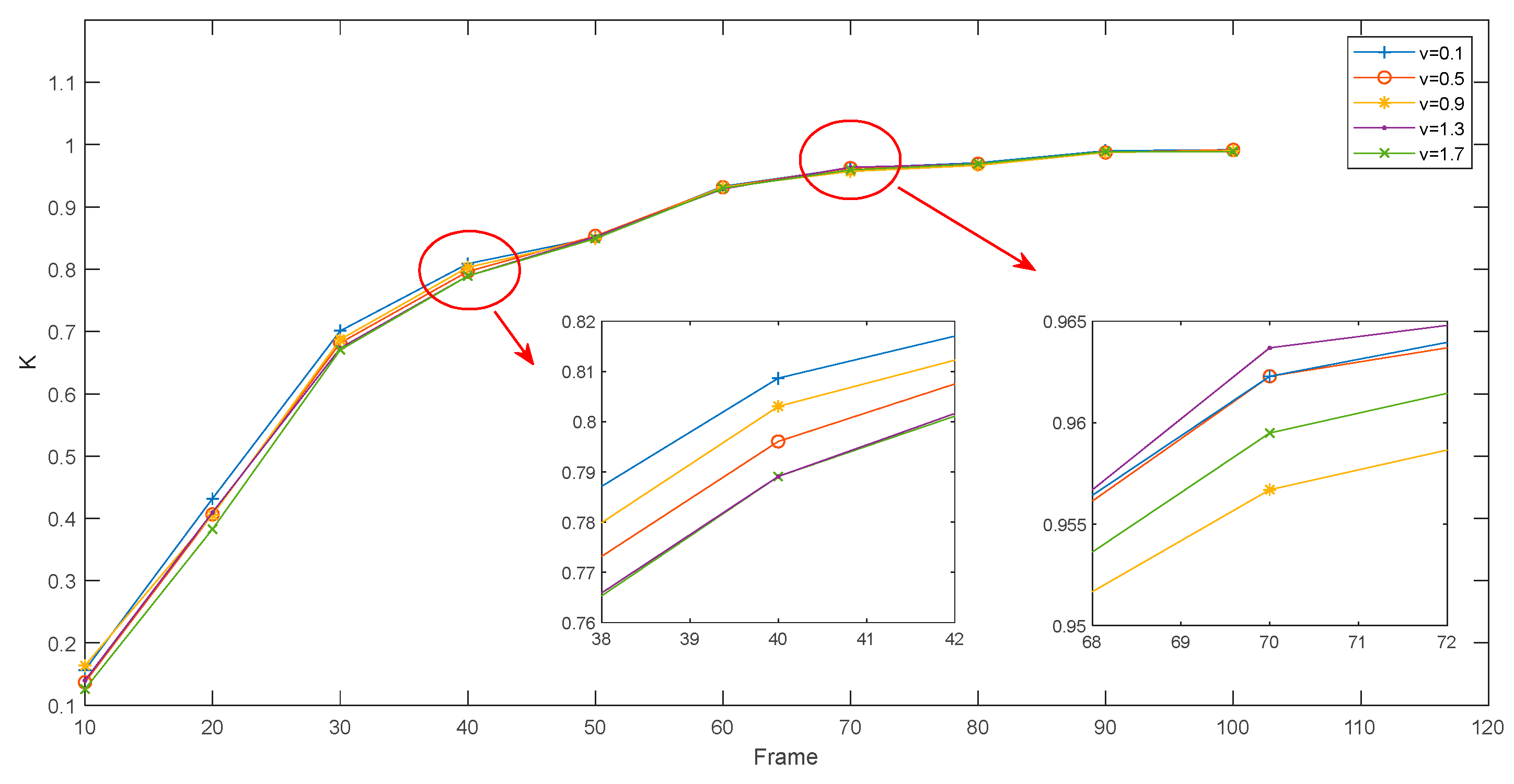
| Statistical Frame Numbers | Evaluation Metrics | Optimal Order |
|---|---|---|
| 40 | K | 0.1 |
| SSIM | 0.1 | |
| PSNR | 1.7 | |
| 70 | K | 1.3 |
| SSIM | 1.3 | |
| PSNR | 1.7 |
| Number of Frames | 30 | 50 | 70 | ||||||
|---|---|---|---|---|---|---|---|---|---|
| Algorithm | Original image | TV | FOTV | Original image | TV | FOTV | Original image | TV | FOTV |
| K | 0.5000 | 0.5237 | 0.5768 | 0.6885 | 0.7277 | 0.8655 | 0.7612 | 0.7905 | 0.9232 |
| PSNR | 19.6235 | 20.2623 | 23.1700 | 22.4426 | 23.3513 | 28.4516 | 24.1864 | 25.0615 | 29.8380 |
| SSIM | 0.9423 | 0.9463 | 0.9746 | 0.9744 | 0.9774 | 0.9942 | 0.9839 | 0.9861 | 0.9960 |
| Conditions | [8] | Ours |
|---|---|---|
| SBR | 0.12 | 0.1 |
| Frames | 200 | 100 |
| K | 0.95 | 0.9777 |
| PSNR | 20.83 | 33.3639 |
| SSIM | 0.940 | 0.9982 |
| Evaluation Metrics | Peak Picking Method | Spatial-Domain Differential Peak Picking Method |
|---|---|---|
| K | 0.1058 | 0.3051 |
| PSNR | 14.0479 | 17.3686 |
| SSIM | 0.4065 | 0.7637 |
| Evaluation Metric | TV Recovering | FOTV Recovering |
|---|---|---|
| K | 0.2327 | 0.4109 |
| PSNR | 17.3441 | 17.9471 |
| SSIM | 0.7659 | 0.8186 |
Disclaimer/Publisher’s Note: The statements, opinions and data contained in all publications are solely those of the individual author(s) and contributor(s) and not of MDPI and/or the editor(s). MDPI and/or the editor(s) disclaim responsibility for any injury to people or property resulting from any ideas, methods, instructions or products referred to in the content. |
© 2023 by the authors. Licensee MDPI, Basel, Switzerland. This article is an open access article distributed under the terms and conditions of the Creative Commons Attribution (CC BY) license (https://creativecommons.org/licenses/by/4.0/).
Share and Cite
Xie, D.; Wang, X.; Wang, C.; Yuan, K.; Wei, X.; Liu, X.; Huang, T. A Fractional-Order Total Variation Regularization-Based Method for Recovering Geiger-Mode Avalanche Photodiode Light Detection and Ranging Depth Images. Fractal Fract. 2023, 7, 445. https://doi.org/10.3390/fractalfract7060445
Xie D, Wang X, Wang C, Yuan K, Wei X, Liu X, Huang T. A Fractional-Order Total Variation Regularization-Based Method for Recovering Geiger-Mode Avalanche Photodiode Light Detection and Ranging Depth Images. Fractal and Fractional. 2023; 7(6):445. https://doi.org/10.3390/fractalfract7060445
Chicago/Turabian StyleXie, Da, Xinjian Wang, Chunyang Wang, Kai Yuan, Xuyang Wei, Xuelian Liu, and Tingsheng Huang. 2023. "A Fractional-Order Total Variation Regularization-Based Method for Recovering Geiger-Mode Avalanche Photodiode Light Detection and Ranging Depth Images" Fractal and Fractional 7, no. 6: 445. https://doi.org/10.3390/fractalfract7060445