
Study Models of COVID-19 in Discrete-Time and Fractional-Order

 ,
,  , , and
Abstract
:1. Introduction
2. Preliminaries
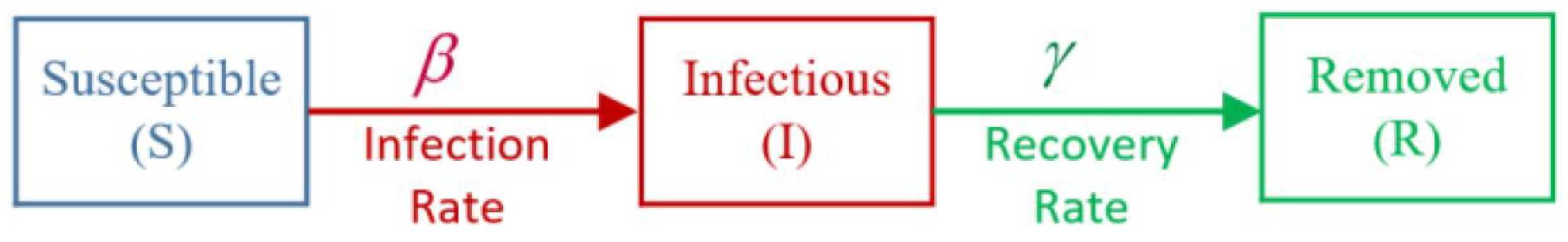
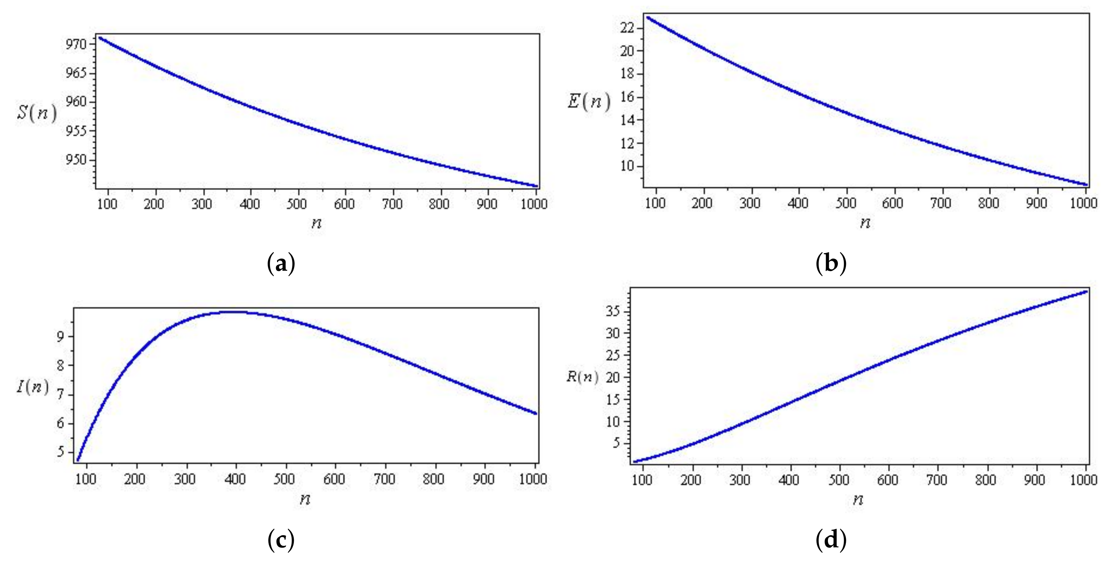
3. SIR Model
3.1. SIR Model as a Continuous Time
3.2. SIR Model as a Discrete Time
3.3. Fixed Points
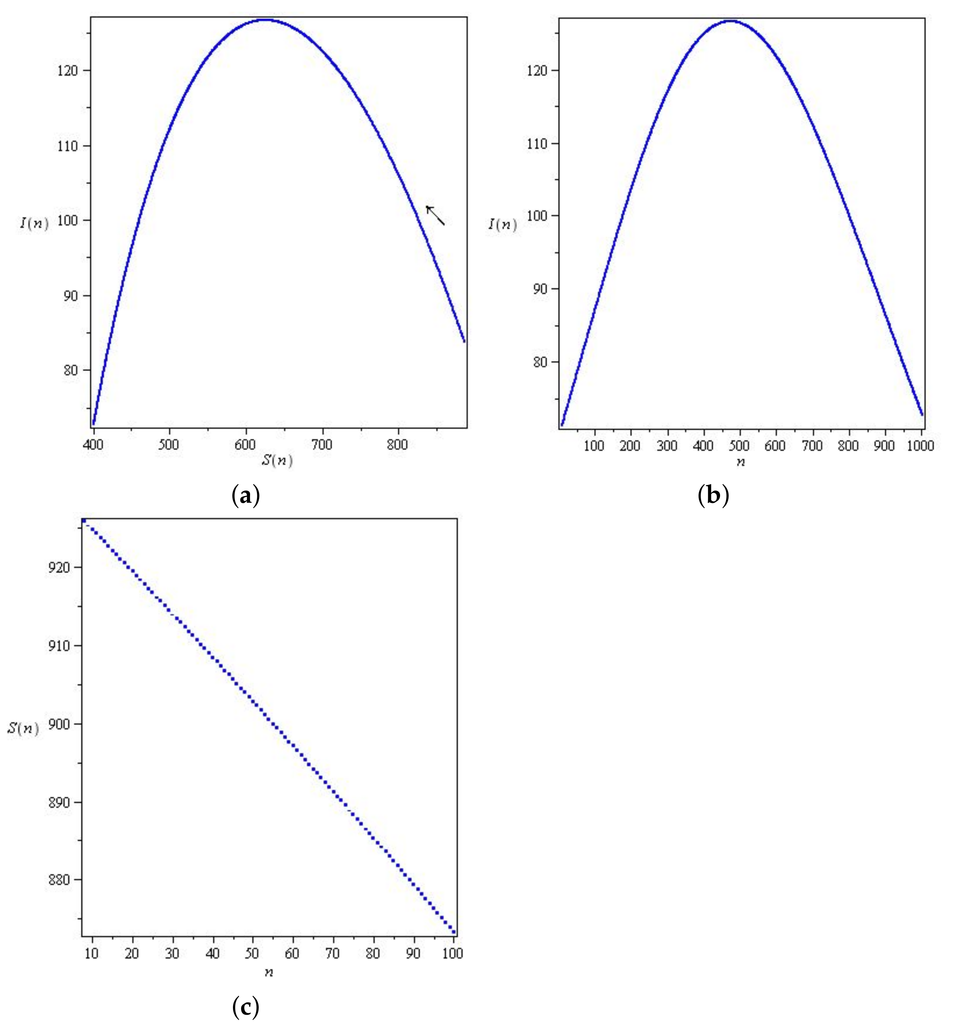
3.4. Orbits
3.5. Stability Analysis for the Discrete Sir System
3.6. Fractional-Order SIR System and Discretization
3.7. Fixed Points and Stability
- If or , then , and the fixed point is an unstable node.
- If or , then and the fixed point is a saddle.
- If and , then the fixed point is an unstable node.
- If and , then the fixed point is a saddle.
- If and , then the fixed point is an unstable spiral node.
- If and , then the fixed point is a saddle-spiral.
3.8. Determining and for Model (26) at a Discrete Time from the Observed Data
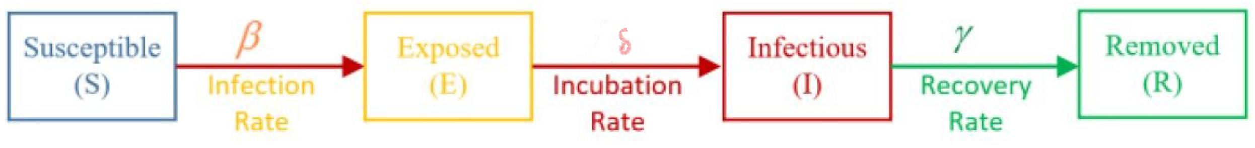
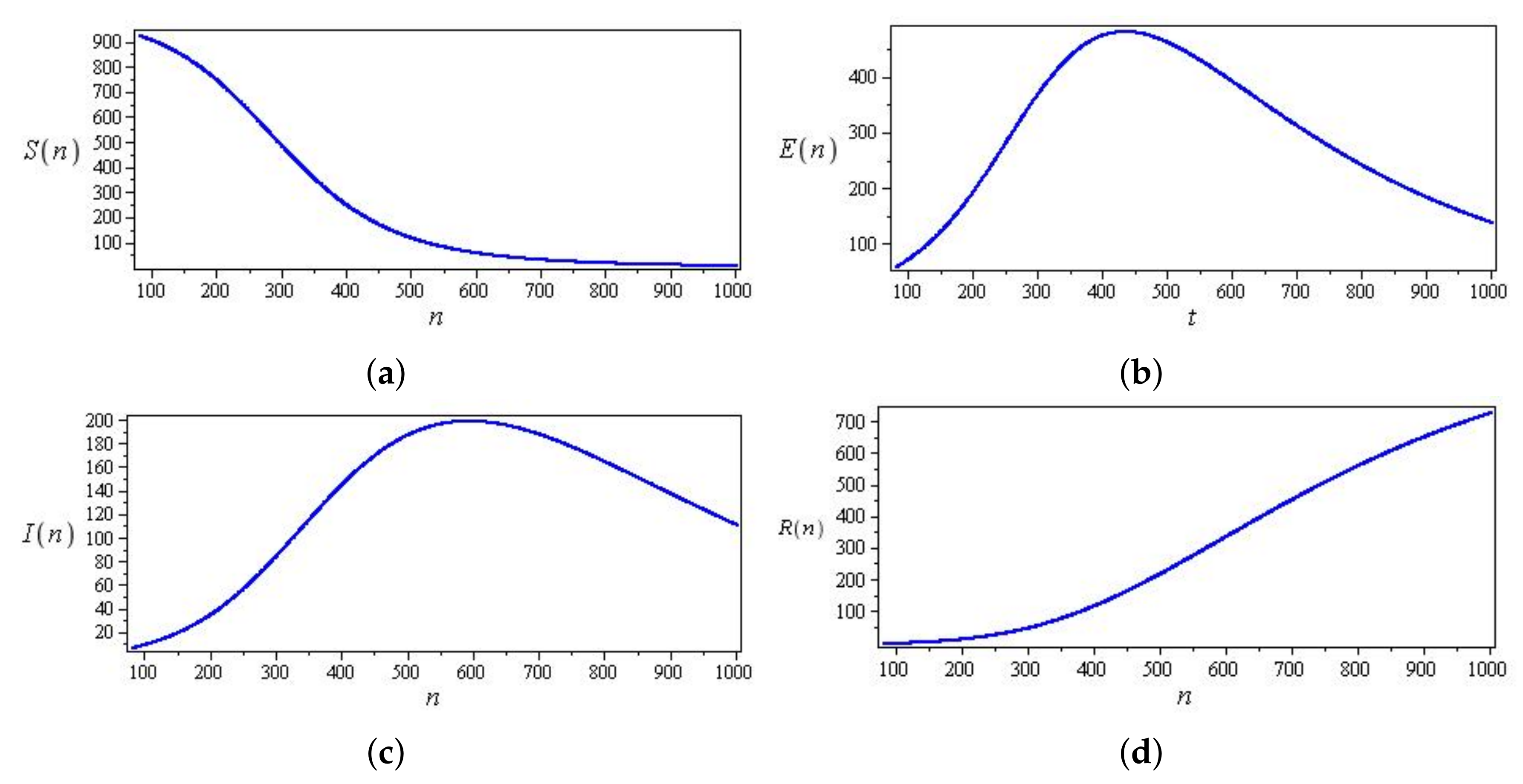
4. SEIR Model
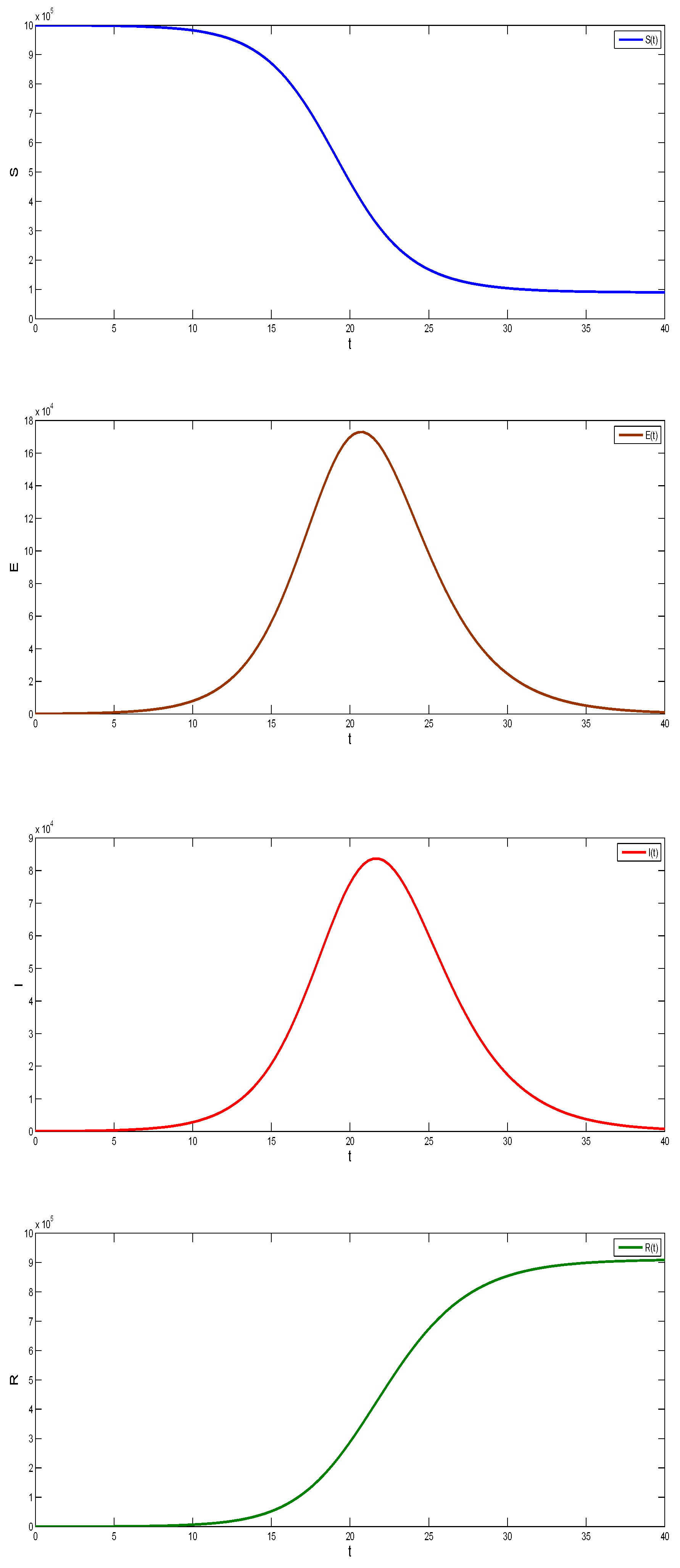
4.1. SEIR Model as a Continuous Time
4.2. SEIR Model as a Discrete Time
4.3. Fixed Points
4.4. Fractional Order SEIR System and Discretization
4.5. Fixed Points and Stability
4.6. Determining and for Model (59) at a Discrete Time from the Observed Data
5. Results
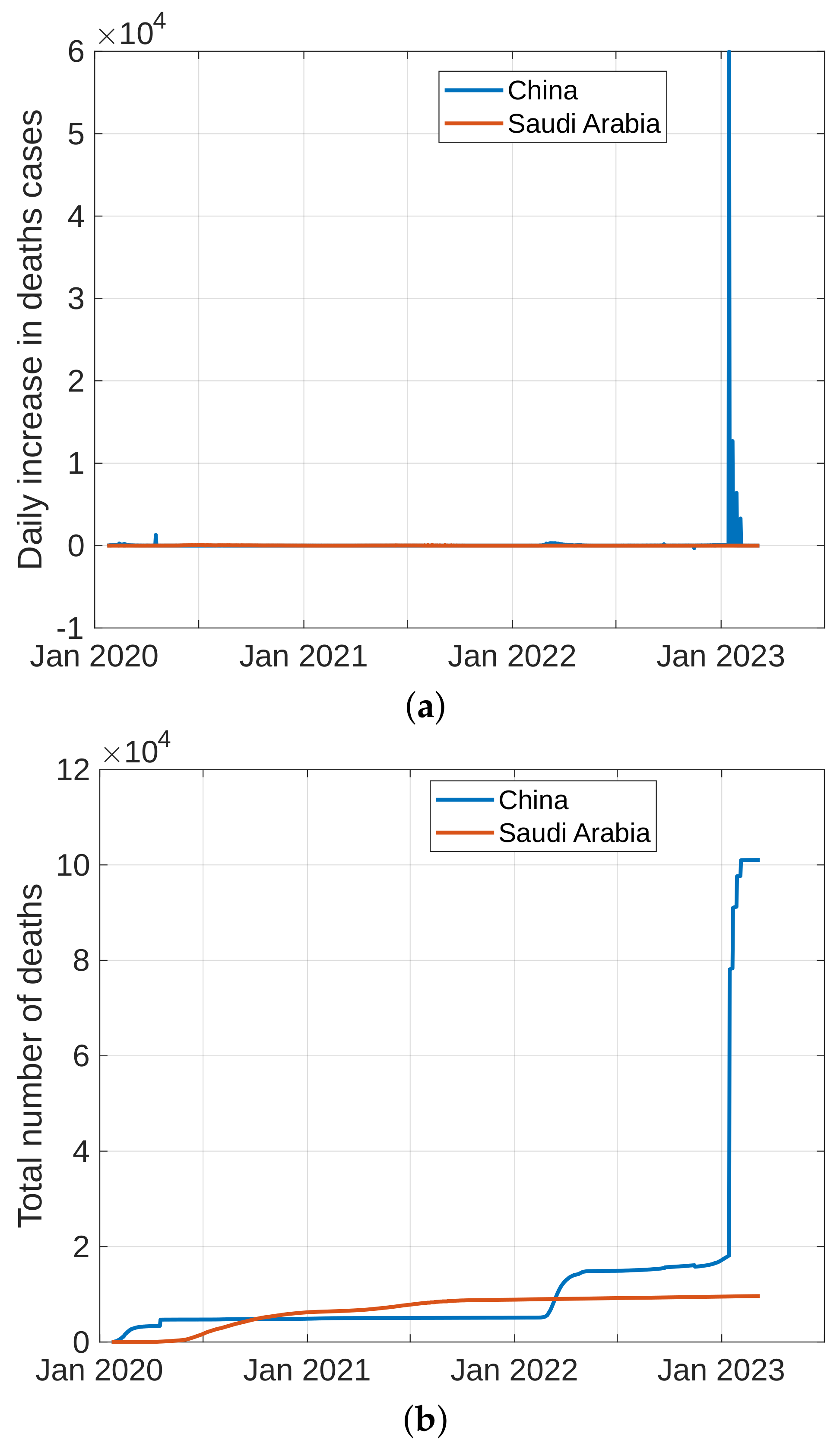
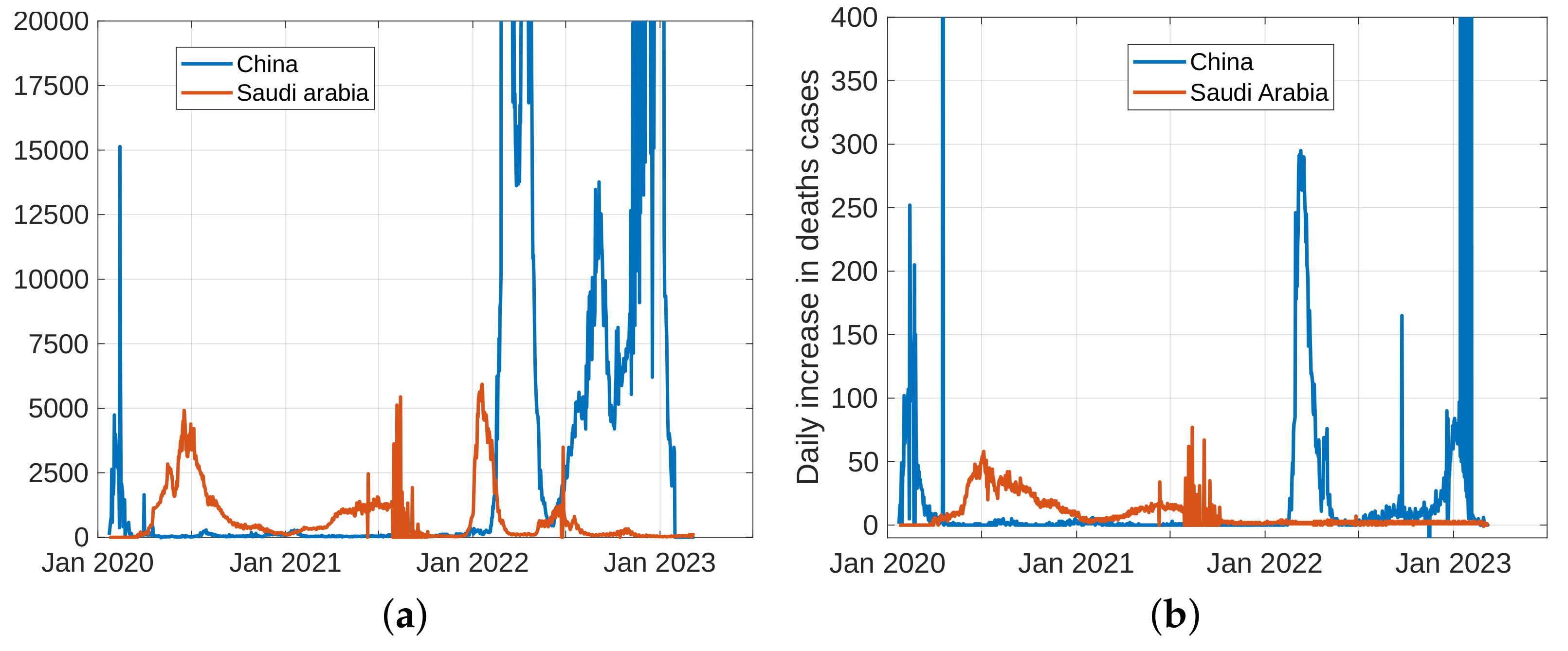
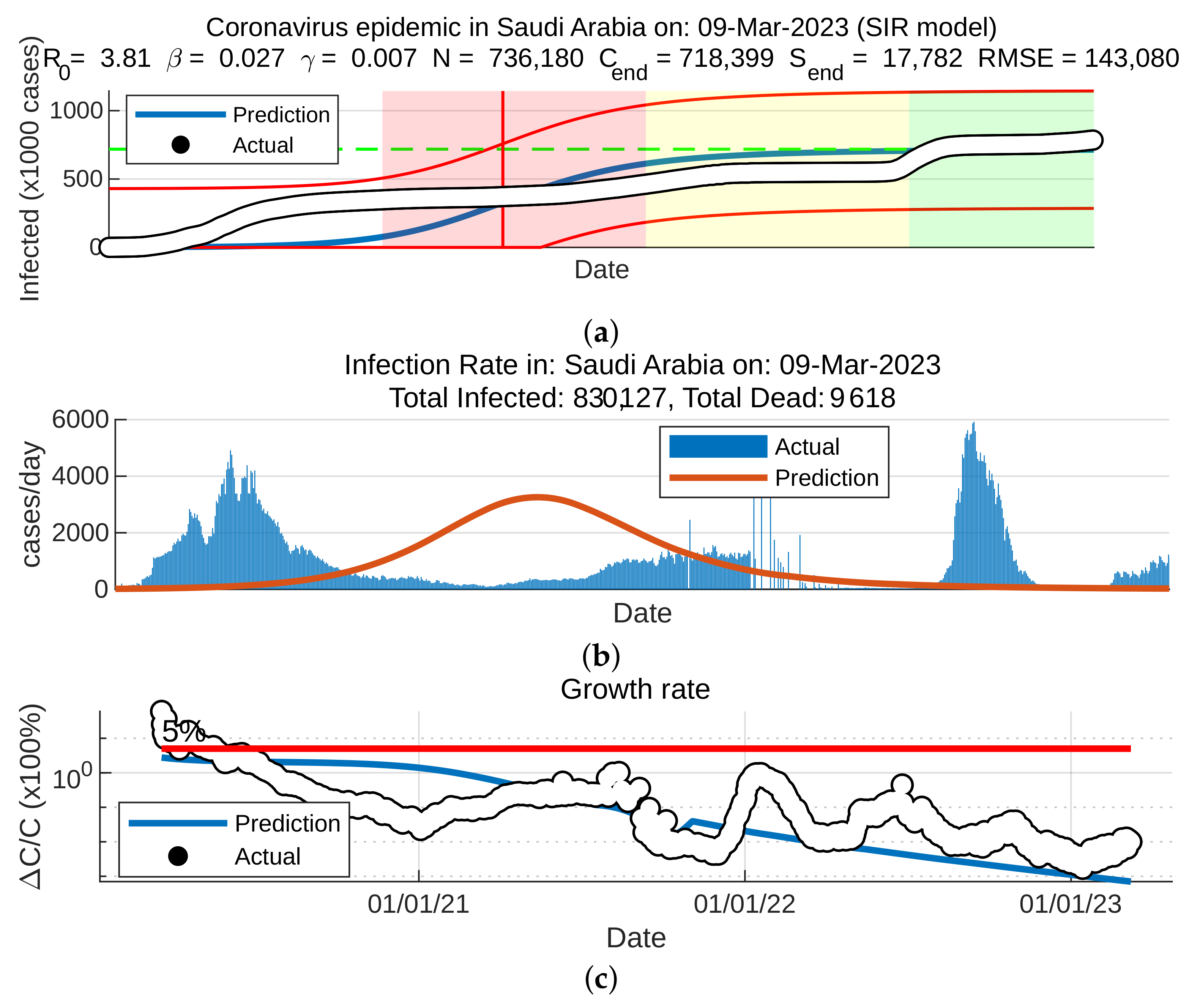
5.1. Coronavirus (COVID-19) Outbreaks in China and Saudi Arabia 2022
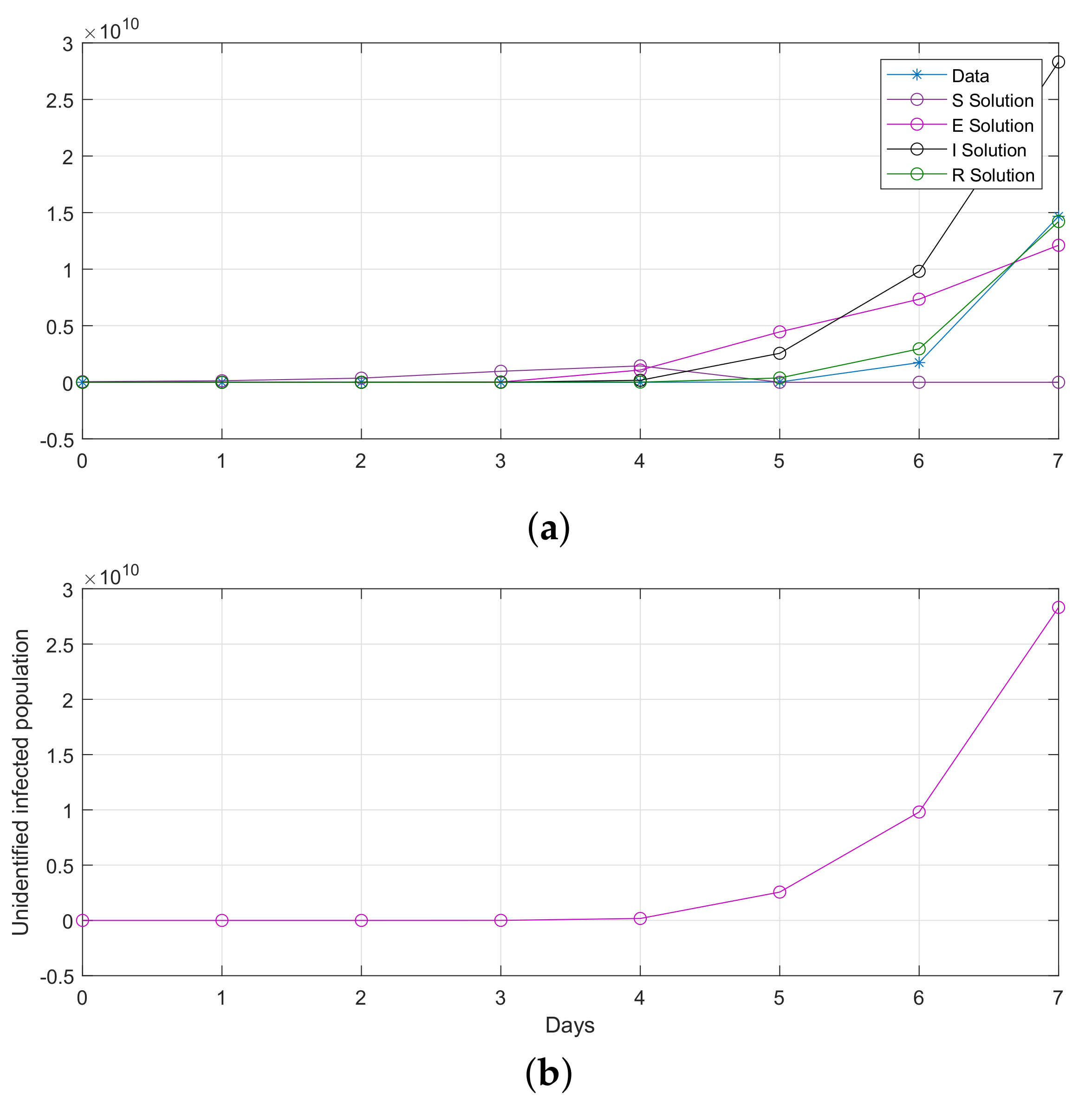
5.2. Results for the SIR and SEIR Systems Using the Data
6. Conclusions
Author Contributions
Funding
Data Availability Statement
Acknowledgments
Conflicts of Interest
References
- Liu, Y.C.; Kuo, R.L.; Shih, S.-R. COVID-19: The first documented coronavirus pandemic in history. Biomed. J. 2020, 43, 328–333. [Google Scholar] [CrossRef] [PubMed]
- Majumder, M.; Mandl, K.D. Early transmissibility assessment of a novel coronavirus in Wuhan, China. SSRN Electron. J. 2020. [Google Scholar] [CrossRef]
- Mtewa, A.G.; Amanjot, A.; Yadesa, T.M.; Ngwira, K.J. Drug repurposing for SARS-COV-2 (COVID-19) treatment. Coronavirus Drug Discov. 2022, 1, 205–226. [Google Scholar] [CrossRef]
- Yang, J.; Gong, H.; Chen, X.; Chen, Z.; Deng, X.; Qian, M.; Hou, Z.; Ajelli, M.; Viboud, C.; Yu, H. Review for health-seeking behaviors of patients with acute respiratory infections during the outbreak of novel Coronavirus Disease 2019 in Wuhan, China. Influenza Other Respir. Viruses 2020, 15, 188–194. [Google Scholar] [CrossRef] [PubMed]
- Segel, L.A.; Murray, J.D. Mathematical Biology (3rd ed), Volume I (An Introduction) and Volume II (Spatial models and biomedical applications). Math. Med. Biol. 2003, 20, 377–378. [Google Scholar] [CrossRef]
- Srinivasan, S.; Cui, H.; Gao, Z.; Liu, M.; Lu, S.; Mkandawire, W.; Narykov, O.; Sun, M.; Korkin, D. Structural genomics of SARS-COV-2 indicates evolutionary conserved functional regions of viral proteins. Viruses 2020, 12, 360. [Google Scholar] [CrossRef]
- Liu, D.X.; Liang, J.Q.; Fung, T.S. Human Coronavirus-229E, -OC43, -NL63, and -HKU1 (Coronaviridae). Encycl. Virol. 2021, 428–440. [Google Scholar] [CrossRef]
- Zhao, S.; Lin, Q.; Ran, J.; Musa, S.S.; Yang, G.; Wang, W.; Lou, Y.; Gao, D.; Yang, L.; He, D.; et al. Preliminary estimation of the basic reproduction number of novel coronavirus (2019-ncov) in China, from 2019 to 2020: A data-driven analysis in the early phase of the outbreak. Int. J. Infect. Dis. 2020, 92, 214–217. [Google Scholar] [CrossRef]
- Data Source COVID-19: Center for Systems Science and Engineering (CSSE) at Johns Hopkins University (JHU). Available online: https://coronavirus.jhu.edu/region/ (accessed on 8 April 2023).
- Msmali, A.; Mutum, Z.; Mechai, I.; Ahmadini, A. Modeling and simulation: A study on predicting the outbreak of COVID-19 in Saudi Arabia. Discret. Dyn. Nat. Soc. 2021, 2021, 5522928. [Google Scholar] [CrossRef]
- Data Source COVID-19: World Health Organization (WHO). Available online: https://covid19.who.int/data (accessed on 8 April 2023).
- Rangasamy, M.; Chesneau, C.; Martin-Barreiro, C.; Leiva, V. On a novel dynamics of SEIR epidemic models with a potential application to COVID-19. Symmetry 2022, 14, 1436. [Google Scholar] [CrossRef]
- Verma, H.; Mishra, V.N.; Mathur, P. Effectiveness of lock down to curtail the spread of Corona virus: A mathematical model. ISA Trans. 2022, 124, 124–134. [Google Scholar] [CrossRef] [PubMed]
- Saeed, T.; Djeddi, K.; Guirao, J.L.; Alsulami, H.H.; Alhodaly, M.S. A discrete dynamics approach to a tumor system. Mathematics 2022, 10, 1774. [Google Scholar] [CrossRef]
- De Natale, G.; Ricciardi, V. The COVID-19 infection in Italy: A statistical study of an abnormally severe disease. J. Clin. Med. 2020, 9, 1564. [Google Scholar] [CrossRef] [PubMed]
- Frank, T.D. COVID-19 Epidemiology and Virus Dynamics Nonlinear Physics and Mathematical Modeling; Springer: Berlin/Heidelberg, Germany, 2022. [Google Scholar]
- Kurmi, S.; Chouhan, U. A multicompartment mathematical model to study the dynamic behavior of COVID-19 using vaccination as control parameter. Nonlinear Dyn. 2022, 109, 2185–2201. [Google Scholar] [CrossRef] [PubMed]
- Mihailo, P.L.; Milan, R.R.; Tomislav, B.S. Introduction to Fractional Calculus with Brief Historical Background. 2014. Available online: https://www.researchgate.net/publication/312137269_Introduction_to_Fractional_Calculus_with_Brief_Historical_Background (accessed on 10 April 2023).
- Xu, C.; ur Rahman, M.; Baleanu, D. On fractional-order symmetric oscillator with offset-boosting control. Nonlinear Anal. Model. Control. 2022, 27, 1–15. [Google Scholar] [CrossRef]
- Khan, F.S.; Khalid, M.; Al-moneef, A.A.; Ali, A.H.; Bazighifan, O. Freelance model with Atangana–Baleanu Caputo fractional derivative. Symmetry 2022, 14, 2424. [Google Scholar] [CrossRef]
- Hamdan, N.I.; Kilicman, A. A fractional order sir epidemic model for dengue transmission. Chaos Solitons Fractals 2018, 114, 55–62. [Google Scholar] [CrossRef]
- Kamel, D. Dynamics in a Discrete—Time Three Dimensional Cancer System. Int. J. Appl. Math. 2019, 49, 1–7. [Google Scholar]
- Khennaoui, A.; Ouannas, A.; Bendoukha, S.; Grassi, G.; Lozi, R.P.; Pham, V. On fractional–order discrete–time systems: Chaos, stabilization and synchronization. Chaos Solitons Fractals 2019, 119, 150–162. [Google Scholar] [CrossRef]
- Abdulrahman, I. Simcovid: Open-source simulation programs for the COVID-19 Outbreak. Comput. Sci. 2022, 4, 20. [Google Scholar] [CrossRef]
- Chen, T.-M.; Rui, J.; Wang, Q.-P.; Zhao, Z.-Y.; Cui, J.-A.; Yin, L. A mathematical model for simulating the phase-based transmissibility of a novel coronavirus. Infect. Dis. Poverty 2020, 9, 24. [Google Scholar] [CrossRef]
- Data Source COVID-19: CSSEGISandData. (n.d.). CSSEGISANDDATA/COVID-19: Novel coronavirus (COVID-19) Cases, Provided by JHU CSSE. GitHub. Available online: https://github.com/CSSEGISandData/COVID-19 (accessed on 8 April 2023).
- Kermack, W.O.; McKendrick, A.G. A Contribution to the Mathematical Theory of Epidemics; Royal Society: London, UK, 1927; Volume 115. [Google Scholar] [CrossRef]
- Muñoz-Fernández, G.A.; Seoane, J.M.; Seoane-Sepúlveda, J.B. A sir-type model describing the successive waves of COVID-19. Chaos Solitons Fractals 2021, 144, 110682. [Google Scholar] [CrossRef] [PubMed]
- Angstmann, C.N.; Henry, B.I.; McGann, A.V. A fractional-order infectivity and Recovery Sir Model. Fractal Fract. 2017, 1, 11. [Google Scholar] [CrossRef]
- Singh, R.A.; Lal, R.; Kotti, R.R. Time-discrete SIR model for COVID-19 in Fiji. In Epidemiology and Infection; Cambridge University Press: Cambridge, MA, USA, 2022; Volume 150. [Google Scholar] [CrossRef]
- Wacker, B.; Schlüter, J. Time-continuous and time-discrete SIR models revisited: Theory and applications. Adv. Differ. Equ. 2020, 2020, 556. [Google Scholar] [CrossRef]
- Metcalfe, C. Book review: Pan J-X, Fang K-T 2002: Growth curve models and statistical diagnostics. In Statistical Methods in Medical Research; Springer: New York, NY, USA, 2007; Volume 59, pp. 341–342. ISBN 0-387-95053-2. [Google Scholar] [CrossRef]
- Su, S. Maximum Log Likelihood Estimation using EM Algorithm and Partition Maximum Log Likelihood Estimation for Mixtures of Generalized Lambda Distributions. J. Mod. Appl. Stat. Methods 2011, 10, 599–606. [Google Scholar] [CrossRef]
- Dai, Y.; Billard, L. Maximum likelihood estimation in space time bilinear models. J. Time Ser. Anal. 2003, 24, 25–44. [Google Scholar] [CrossRef]
- Salgotra, R.; Gandomi, M.; Gandomi, A.H. Time Series Analysis and Forecast of the COVID-19 Pandemic in India using Genetic Programming. Chaos Solitons Fractals 2020, 138, 109945. [Google Scholar] [CrossRef]
- Willmott, C.; Matsuura, K. Advantages of the mean absolute error (MAE) over the root mean square error (RMSE) in assessing average model performance. Clim. Res. 2005, 30, 79–82. [Google Scholar] [CrossRef]
- He, Z.Y.; Abbes, A.; Jahanshahi, H.; Alotaibi, N.D.; Wang, Y. Fractional-order discrete-time sir epidemic model with vaccination: Chaos and complexity. Mathematics 2022, 10, 165. [Google Scholar] [CrossRef]
- Gu, Y.; Khan, M.A.; Hamed, Y.S.; Felemban, B.F. A comprehensive mathematical model for SARS-COV-2 in Caputo derivative. Fractal Fract. 2021, 5, 271. [Google Scholar] [CrossRef]
- Ahmadini, A.; Msmali, A.; Mutum, Z.; Raghav, Y.S. The Mathematical Modeling Approach for the wastewater treatment process in Saudi Arabia during COVID-19 pandemic. Discret. Dyn. Nat. Soc. 2022, 2022, 1061179. [Google Scholar] [CrossRef]
- Lin, Q.; Chiu, A.P.Y.; Zhao, S.; He, D. Modeling the spread of Middle East respiratory syndrome coronavirus in Saudi Arabia. Stat. Methods Med. Res. 2018, 27, 1968–1978. [Google Scholar] [CrossRef] [PubMed]


Disclaimer/Publisher’s Note: The statements, opinions and data contained in all publications are solely those of the individual author(s) and contributor(s) and not of MDPI and/or the editor(s). MDPI and/or the editor(s) disclaim responsibility for any injury to people or property resulting from any ideas, methods, instructions or products referred to in the content. |
© 2023 by the authors. Licensee MDPI, Basel, Switzerland. This article is an open access article distributed under the terms and conditions of the Creative Commons Attribution (CC BY) license (https://creativecommons.org/licenses/by/4.0/).
Share and Cite
Djeddi, K.; Bouali, T.; Msmali, A.H.; Ahmadini, A.A.H.; Koam, A.N.A. Study Models of COVID-19 in Discrete-Time and Fractional-Order. Fractal Fract. 2023, 7, 446. https://doi.org/10.3390/fractalfract7060446
Djeddi K, Bouali T, Msmali AH, Ahmadini AAH, Koam ANA. Study Models of COVID-19 in Discrete-Time and Fractional-Order. Fractal and Fractional. 2023; 7(6):446. https://doi.org/10.3390/fractalfract7060446
Chicago/Turabian StyleDjeddi, Kamel, Tahar Bouali, Ahmed H. Msmali, Abdullah Ali H. Ahmadini, and Ali N. A. Koam. 2023. "Study Models of COVID-19 in Discrete-Time and Fractional-Order" Fractal and Fractional 7, no. 6: 446. https://doi.org/10.3390/fractalfract7060446