On the Roots of a Family of Polynomials

Abstract

The aim of this paper is to give a characterization of the set of roots of a special family of polynomials. This family is relevant in reliability theory since it contains the reliability polynomials of the networks created by series-parallel compositions. We prove that the set of roots is bounded, being contained in the two disks of the radius equal to the golden ratio, centered at 0 and at 1. We study the closure of the set of roots and prove that it includes two disks centered at 0 and 1 of a radius slightly greater than 1, as well as the sinusoidal spirals centered at 0 and at 1, respectively. The expression of some limit points is also provided.

1. Introduction

The location of the roots of polynomials has always been a subject of interest, starting from the very moment when Gauss introduced the geometric representation of complex numbers as points in the plane. One of the early results in this area was given by Cauchy, who proved (see [1]) that all of the roots of a polynomial with complex coefficients $f\left(z\right)={\displaystyle \sum _{k=0}^n}{a}_k{z}^k$ lie in the disk

$$\left|z\right|\le 1+\underset{0\le k\le n}{max}\left|\frac{a_k}{a_n}\right|.$$

Another important result concerning the roots of a polynomial with positive coefficients is the Eneström-Kakeya Theorem (see [2,3]), which states that if $0<a_0\le a_1\le \dots \le a_n$, then the roots of the polynomial $f\left(z\right)={\displaystyle \sum _{k=0}^n}{a}_k{z}^k$ lie in the disk $\left|z\right|\le 1$. An equivalent (but more useful) statement of the theorem (see [4,5]) is that the roots of the polynomial $f\left(z\right)$ with positive coefficients lie in the annulus

$$\underset{1\le k\le n}{min}\frac{a_{k-1}}{a_k}\le \left|z\right|\le \underset{1\le k\le n}{max}\frac{a_{k-1}}{a_k}.$$

Besides the theoretical significance, the study of polynomial zeros has important applications in various domains such as control theory, signal processing, and network reliability theory. From a mathematical point of view, a network is an undirected graph with perfectly reliable nodes, with each edge independently operational with some probability $p\in [0,1]$. Introduced by Moore and Shannon in 1956 [6], the two-terminal reliability of a network is the probability that two specified nodes s and t (called terminals) are connected by a path made of operational edges, while the all-terminal reliability is the probability that any two nodes are connected by such a path [7,8]. In both cases, the reliability is a polynomial function in p.

Since it measures the robustness of a network, the reliability polynomial has become a very important research topic in recent decades. The combinatorial problem of calculating the reliability of a network has been proved to belong to the class of $\#P$-complete problems [9], which means that the time of calculation exponentially increases with the size of the network. Therefore, the research in the field has mainly concentrated in two directions: the first direction aims at finding methods to approximate the reliability polynomial (see, for example [10,11,12,13,14,15]), while the other one studies the analytic properties of these polynomials, such as shape (convexity, inflection points) on the one hand [16,17,18,19] and roots (real or complex) on the other [20,21,22,23].

The roots of all-terminal reliability polynomials have been intensively studied, using the Eneström-Kakeya Theorem. In 1992, Brown and Colbourn conjectured that these roots lie inside the disk $|z-1|\le 1$ [20]. The conjecture was proved to be false twelve years later [24], but the roots found outside the disk are still close to the circle $|z-1|=1$. Although two-terminal reliability polynomials have many features in common with all-terminal reliability polynomials, their roots seem to behave quite differently. Recently, Brown and deGagné [21,23] have proved that the closure of the roots of two-terminal reliability polynomials contains the disks $\left|z\right|\le 1$ and $|z-1|\le 1$ and that real roots approaching $-\varphi$ and $1+\varphi$ exist (where $\varphi =\frac{1+\sqrt{5}}{2}$ is the golden ratio).

By taking a broader view, we remark that the reliability polynomial is just one of the polynomials associated with a graph. Another famous graph polynomial is the chromatic polynomial ${\mathcal{C}}_G\left(k\right)$ used to describe the number of ways to color the vertices of a graph G with a given number of colors k so that no two adjacent vertices have the same color. The chromatic polynomial was introduced by Birkhoff in 1912 [25] in the hope that the study of the real or complex zeros of ${\mathcal{C}}_G\left(z\right)$ might lead to an analytic proof of the four-color conjecture, which states that ${\mathcal{C}}_G\left(4\right)>0$ for any planar graph G. Although this hope has not been realized, the zeros of ${\mathcal{C}}_G\left(z\right)$ (called chromatic roots) have become a subject of great interest for scientists [26,27,28,29]. A remarkable theorem proved by Sokal [28] states that the set of chromatic roots is dense in the complex plane, while Jackson [27] and Thomassen [29] proved that the closure of the real chromatic roots is the set $\{0,1\}\cup [32/27,\infty )$.

Similar results have been demonstrated for two other (“younger”) polynomials: the independence polynomials and the domination polynomials. The independence polynomial ${\mathcal{I}}_G\left(x\right)$ was defined by Gutman and Harary in 1983 [30] as ${\mathcal{I}}_G\left(x\right)=\sum s_k{x}^k$, where $s_k$ is the number of independent k-sets (an independent set in a graph is a set of pairwise non-adjacent vertices). Brown et al. [31] proved that real roots of independence polynomials are dense in $(-\infty ,0]$, while complex roots are dense in $\mathbb{C}$. The roots of independence polynomials (called independence roots) continue to be a highly interesting area of research (see, for instance, [32]).

Introduced by Arocha and Llano [33] just two decades ago, the domination polynomials have quickly become an attractive topic for researchers in the field [34,35,36,37]. A dominating set of a graph G is a set of vertices S such that every vertex that is not in S is adjacent to a vertex of S. The domination polynomial is defined by the formula ${\mathcal{D}}_G\left(x\right)=\sum d_k{x}^k$, where $d_k$ is the number of dominating sets with k elements. The complex roots of these polynomials (domination roots) were proved to be also dense in the complex plane [37], while the closure of the real roots is $(-\infty ,0]$ [34].

The main contributions of the paper are as follows:

• We introduce the family $\mathcal{F}$ of polynomials obtained by composing the elementary polynomials $g\left(x\right)=1-x$ and ${\phi }_n\left(x\right)=x^n$.
• We prove that the set of roots of this infinite family of polynomials is bounded by the circles $\left|z\right|=\varphi$ and $|z-1|=\varphi$. A direct consequence is that the roots of the reliability polynomials of series-parallel composition networks are bounded.
• Starting from the result proved by Brown and deGagné [21,23], we show that the closure of the set of roots of the polynomials in $\mathcal{F}$ contains the domain bounded by the lemniscates with n poles centered at 0 and at 1; hence, it contains two disks of radius slightly greater than 1, centered at 0 and at 1.
• We find 16 complex limit points of the set of roots apart from $-\varphi$ and $1+\varphi$, the two limit points on the real axis noted in [21].

The paper is organized in 6 sections (including this introductory section). Section 2 introduces the family $\mathcal{F}$ of polynomials and describes their basic properties. In Section 3, we prove that the roots of these polynomials are bounded by the two circles of radius $\varphi$ centered at 0 and at 1. Section 4 is devoted to the closure of the set of roots $\overline{\mathcal{S}}$, while Section 5 establishes a number of limit points of the set of roots. The conclusions and some open problems raised by the paper are presented in Section 6.

2. Preliminaries

An important class of two-terminal networks are those obtained by series-parallel compositions (see [22,38,39,40]). The reliability of a network consisting of n identical edges connected in series, each one independently working with the probability p, is $p^n$, while the reliability of a network with n edges connected in parallel is $1-{(1-p)}^n$. Therefore, it is quite natural to consider the family of polynomials obtained by composing the polynomials:

$$\begin{array}{cc}\hfill {\phi }_n\left(x\right)& =x^n,n=2,3,\dots ,\hfill \\ \hfill g\left(x\right)& =1-x.\hfill \end{array}$$

The aim of the paper is to provide a characterization of the set of roots of these polynomials.

First of all, we notice that $g=g^{-1}$ and ${\phi }_m\circ {\phi }_n={\phi }_{mn}$ for any $m,n\ge 2$. We also remark that for any polynomial f and every $n\ge 2$, the polynomial ${\phi }_n\circ f$ has the same roots as f. Thus, using for composition the notation $fg=f\circ g$, we define the family of polynomials $\mathcal{F}={\mathcal{F}}_0\cup {\mathcal{F}}_1$, where ${\mathcal{F}}_0$ and ${\mathcal{F}}_1$ are the disjoint sets

$$\begin{array}{cc}\hfill {\mathcal{F}}_0& =\{f=g{\phi }_{n_1}\dots g{\phi }_{n_k}:n_j\ge 2,j=1\dots k,k\ge 1\},\hfill \\ \hfill {\mathcal{F}}_1& =\{f=g{\phi }_{n_1}\dots g{\phi }_{n_k}g:n_j\ge 2,j=1\dots k,k\ge 1\}.\hfill \end{array}$$

Not every polynomial of the family $\mathcal{F}$ is the reliability polynomial of some network created by series-parallel composition. The reliability polynomials of such networks are the members of ${\mathcal{F}}_0$ with k even, and the members of ${\mathcal{F}}_1$ with k odd (in other words, the compositions where the polynomial g has an even number of occurrences).

Consider, for instance, the series-parallel network ${\mathcal{N}}_{m,n}$ consisting of m internally disjoint paths (each of length n) connecting the two vertices s and t. If each edge is operational with some probability $x\in [0,1]$, then the reliability polynomial of the network (the probability that the two terminals s and t are connected by at least one operational path) is

$$f_{m,n}\left(x\right)=1-{(1-x^n)}^m=g{\phi }_{m}g{\phi }_n\left(x\right).$$

(1)

Suppose that k such networks are connected in series to form a more complex network, ${\mathcal{N}}_{k,m,n}$. The reliability polynomial of this network is

$$f_{k,m,n}\left(x\right)={\left(1-{(1-x^n)}^m\right)}^k={\phi }_{k}g{\phi }_{m}g{\phi }_n\left(x\right),$$

(2)

and its roots are the same as the roots of $f_{m,n}\left(x\right)$.

Let $\mathcal{S}$ denote the set of all roots of the polynomials in $\mathcal{F}$ and, for every $k=1,2,\dots$, we denote by $L_k$ and $R_k$, respectively, the following sets of roots:

$$\begin{array}{cc}\hfill L_k& =\{z\in \mathbb{C}:\exists n_1,\dots ,n_k\ge 2s.t.g{\phi }_{n_1}\dots g{\phi }_{n_k}\left(z\right)=0\},\hfill \end{array}$$

(3)

$$\begin{array}{cc}\hfill R_k& =\{z\in \mathbb{C}:\exists n_1,\dots ,n_k\ge 2s.t.g{\phi }_{n_1}\dots g{\phi }_{n_k}g\left(z\right)=0\}.\hfill \end{array}$$

(4)

Obviously, the set $\mathcal{S}$ can be written

$$\mathcal{S}=\underset{k\ge 1}{\cup }(L_k\cup R_k)$$

(5)

and the following properties can be readily proved using the Definitions (3) and (4) of the sets $L_k$ and $R_k$.

Proposition 1.

For every $k\ge 1$, we have:

(i) 

$R_k=1-L_k$ (the sets $R_k$ and $L_k$ are symmetric to each other with respect to $\frac{1}{2}$);

(ii) 

$L_{k+1}=\underset{n\ge 2}{\cup }{\left(g{\phi }_n\right)}^{-1}\left(L_k\right)=\underset{n\ge 2}{\cup }{\phi }_n^{-1}\left(R_k\right)$.

(iii) 

$L_k\subset L_{k+2}$ and $R_k\subset R_{k+2}$, $k=1,2,\dots$.

Proof. 

The first two statements easily follow from the Definitions (3) and (4). We prove (iii):

If $z\in L_k$, then there exists $n_1,\dots ,n_k\ge 2$ such that $g{\phi }_{n_1}\dots g{\phi }_{n_k}\left(z\right)=0.$ It follows that, for any $m,n\ge 2$, we have $g{\phi }_{n}g{\phi }_{m}g{\phi }_{n_1}\dots g{\phi }_{n_k}\left(z\right)=0$; hence, $z\in L_{k+2}$, and we have just proved that $L_k\subset L_{k+2}$. The other inclusion follows by (i). □

We notice that the closure of $L_1$ is the unit circle centered at 0,

$$\overline{L_1}={\mathcal{C}}_0\left(1\right)=\{z\in \mathbb{C}:|z|=1\}$$

and the closure or $R_1=1-L_1$ is the unit circle centered at 1:

$$\overline{R_1}={\mathcal{C}}_1\left(1\right)=\{z\in \mathbb{C}:|z-1|=1\}.$$

As for the real roots, we remark that the polynomials of $\mathcal{F}$ have no real roots in the interval $(0,1)$. As a matter of fact, $f\left(x\right)\in (0,1)$ for any $x\in (0,1)$ and $f\in \mathcal{F}$, and we can prove the following result:

Proposition 2.

Let $f\in \mathcal{F}$, $f=g{\phi }_{n_1}\dots g{\phi }_{n_k}$, where $n_j\ge 2$ for every $j=1,\dots ,k-1$ and $n_k\ge 1$.

(i) 

If k is even then $f\left(0\right)=0$, $f\left(1\right)=1$ and f is strictly increasing on $[0,1]$.

(ii) 

If k is odd then $f\left(0\right)=1$, $f\left(1\right)=0$ and f is strictly decreasing on $[0,1]$.

Proof. 

We notice that $g{\phi }_n\left(0\right)=1$, $g{\phi }_n\left(1\right)=0$, and $g{\phi }_n\left(x\right)\in (0,1)$ for any $x\in (0,1)$ and $n\ge 2$. Since

$$f^{\prime }\left(x\right)={(-1)}^k{n}_1{n}_2\dots n_k{\phi }_{n_1-1}g{\phi }_{n_2}\dots g{\phi }_{n_1}\left(x\right)·{\phi }_{n_2-1}g{\phi }_{n_3}\dots g{\phi }_{n_1}\left(x\right)\dots {\phi }_{n_k-1}\left(x\right),$$

we obtain that, for any $x\in (0,1)$, $f^{\prime }\left(x\right)>0$ if k is even and $f^{\prime }\left(x\right)<0$ if k is odd. □

Remark 1.

Let $f\in \mathcal{F}$, $f=g{\phi }_{n_1}\dots g{\phi }_{n_k}$, where $n_j\ge 2$, $j=1,\dots ,k-1$ and $n_k\ge 1$ if $k\ge 3$, $n_k\ge 2$ if $k=2$. Then, $f^{\prime }\left(0\right)=f^{\prime }\left(1\right)=0$ and so the points $z=0$, $z=1$ are attracting fixed points for f if k is even, or they form an attracting cycle if k is odd (see [41]).

Proposition 3.

If $f=g{\phi }_{n_1}\dots g{\phi }_{n_k}\in {\mathcal{F}}_0$, then its nonzero roots are placed on circles centered at the origin. If $f=g{\phi }_{n_1}\dots g{\phi }_{n_k}g\in {\mathcal{F}}_1$, then its roots different from 1 are placed on circles centered at $z=1$. In both cases, each circle contains $n_k=m$ equally spaced points (but some circles may coincide).

Proof. 

Suppose that $f=g{\phi }_{n_1}\dots g{\phi }_{n_k}$. We denote by $f_1\left(x\right)$ the polynomial

$$f_1\left(x\right)=g{\phi }_{n_1}g{\phi }_{n_2}\dots g{\phi }_{n_{k-1}}g\left(x\right).$$

Let $d_1$ be the degree of $f_1\left(x\right)$, $d_1=n_1{n}_2\dots n_{k-1}$, and let $w_1,\dots ,w_{d_1}\in \mathbb{C}$ be the roots of $f_1\left(x\right)$. If we denote $n_k=m$, the polynomial $f\left(x\right)$ can be written as follows:

$$f\left(x\right)=f_1\left(x^m\right)=\pm \prod _{j=1}^{d_1}(x^m-w_j).$$

Consequently, the nonzero roots of $f\left(x\right)$ are obtained by solving each equation $x^m=w_j$ with $w_j\ne 0$, whose solutions are m equally spaced points on the circle of radius $\sqrt[m]{\left|w_j\right|}$, centered at the origin.

If $f=g{\phi }_{n_1}\dots g{\phi }_{n_k}g$, then $f\left(x\right)=h(1-x)$, where $h\in {\mathcal{F}}_0$. If $z_1,z_2,\dots ,z_d$ are the nonzero roots of h (placed on circles centered at the origin); then, $1-z_1,1-z_2,\dots ,1-z_d$ are the roots of f different from 1 (placed on circles centered at $z=1$). □

3. Bounds for the Set of Roots $\mathcal{S}$

Lemma 1.

Let $z,\zeta \in \mathbb{C}$ such that ${\zeta }^k=z$, where $k\ge 2$ is an integer. If $\left|z-\frac{1}{2}\right|<1+\frac{\sqrt{5}}{2}$, then $\left|\zeta \right|<\frac{1+\sqrt{5}}{2}$.

Proof. 

We have $\left|\zeta \right|=\sqrt[k]{\left|z\right|}$. If $\left|z\right|\le 1$, then $\left|\zeta \right|\le 1<\frac{1+\sqrt{5}}{2}$. Otherwise, if $\left|z\right|>1$, then $\left|\zeta \right|>1$, so we have

$$\left|\zeta \right|=\sqrt[k]{\left|z\right|}\le \sqrt{\left|z\right|}\le \sqrt{\left|z-\frac{1}{2}\right|+\frac{1}{2}}<\sqrt{\frac{3+\sqrt{5}}{2}}=\frac{1+\sqrt{5}}{2}.$$

□

For any $w\in \mathbb{C}$ and $r>0$, we denote by

$$\begin{array}{cc}\hfill {\mathcal{D}}_w\left(r\right)& =\{z\in \mathbb{C}:|z-w|<r\},\hfill \\ \hfill {\overline{\mathcal{D}}}_w\left(r\right)& =\{z\in \mathbb{C}:|z-w|\le r\}\hfill \end{array}$$

the open disk (and the closed disk, respectively) of radius r centered at w.

Theorem 1.

The set of roots $\mathcal{S}$ of the polynomials in $\mathcal{F}$ is contained into the open disk

$${\mathcal{D}}_{1/2}\left(1+\frac{\sqrt{5}}{2}\right)=\left\{z\in \mathbb{C}:\left|z-\frac{1}{2}\right|<1+\frac{\sqrt{5}}{2}\right\}.$$

Proof. 

We prove by mathematical induction on $k\ge 1$ that the roots of any polynomial of the form

$$f\left(x\right)=g{\phi }_{n_1}g{\phi }_{n_2}\dots g{\phi }_{n_k}\left(x\right)$$

are inside the disk ${\mathcal{D}}_{1/2}\left(1+\frac{\sqrt{5}}{2}\right)$.

For $k=1$, the roots of the polynomial $f\left(x\right)=g{\phi }_{n_1}\left(x\right)=1-x^{n_1}$ are the complex roots of unity: $n_1$ equidistant points placed on the circle of radius 1, which is inside the disk ${\mathcal{D}}_{1/2}\left(1+\frac{\sqrt{5}}{2}\right)$.

We suppose that the statement is true for k and prove it for $k+1$. Consider the polynomial

$$f\left(x\right)=g{\phi }_{n_1}g{\phi }_{n_2}\dots g{\phi }_{n_k}g{\phi }_{n_{k+1}}\left(x\right).$$

By the induction hypothesis, the roots $w_1,\dots ,w_n$ of the polynomial

$$f_1\left(x\right)=g{\phi }_{n_1}g{\phi }_{n_2}\dots g{\phi }_{n_k}\left(x\right)$$

are inside the disk ${\mathcal{D}}_{1/2}\left(1+\frac{\sqrt{5}}{2}\right)$. If $n_{k+1}=1$, then

$$f\left(x\right)=f_1(1-x),$$

so the roots of $f\left(x\right)$ are $1-w_1,\dots ,1-w_n$, which are also inside the disk ${\mathcal{D}}_{1/2}\left(1+\frac{\sqrt{5}}{2}\right)$.

If $n_{k+1}=m>1$, then

$$f\left(x\right)=f_1(1-x^m),$$

so the roots of $f\left(x\right)$ are the roots of $x^m=1-w_j$, $j=1,\dots ,n$. Since $1-w_j\in {\mathcal{D}}_{1/2}\left(1+\frac{\sqrt{5}}{2}\right)$, by Lemma 1 it follows that the roots of $f\left(x\right)$ are also inside the disk, and the proof is complete. □

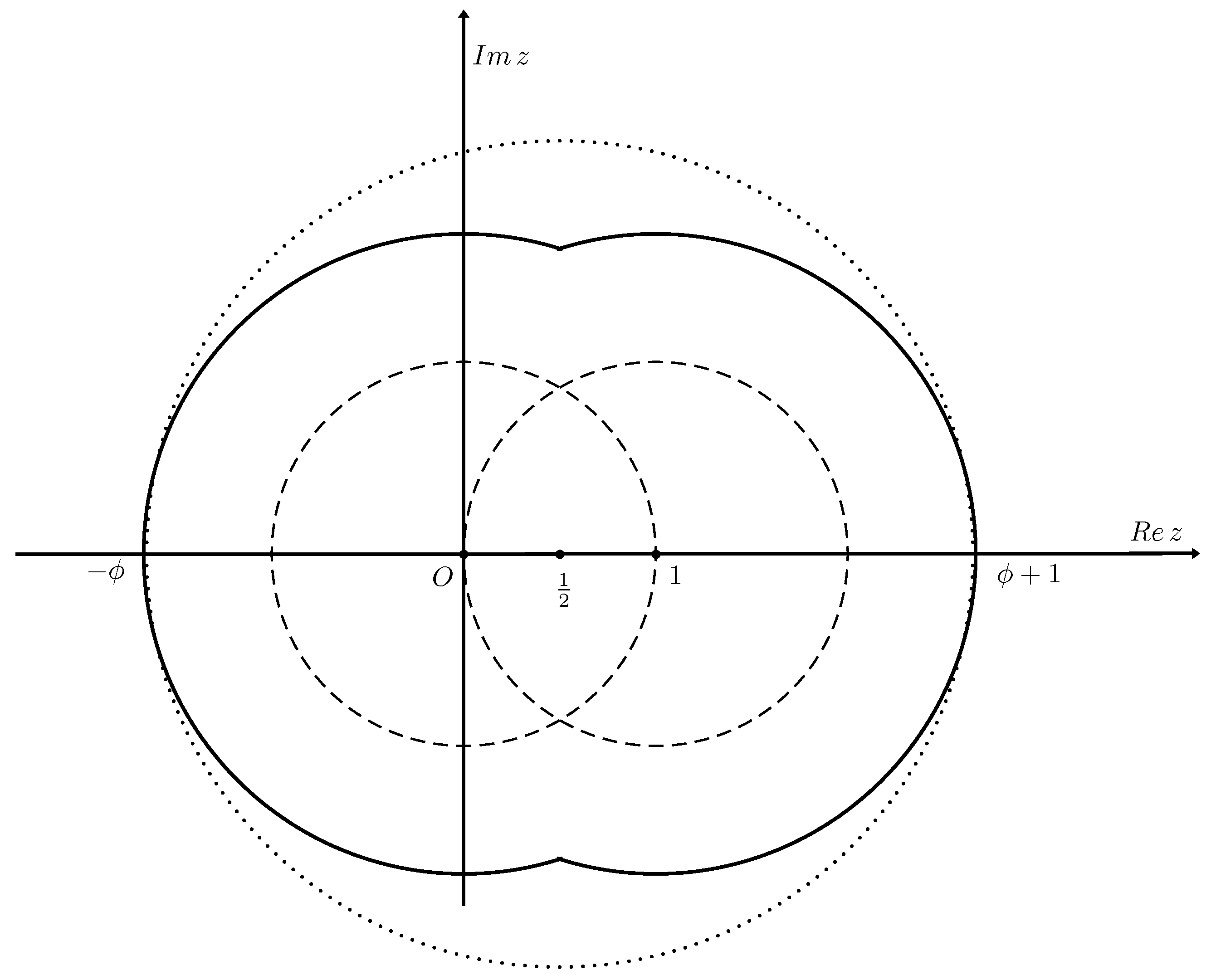
Based on Lemma 1 and Theorem 1, we can find a smaller set containing the set of roots $\mathcal{S}$ (see Figure 1).

Corollary 1.

The set of roots $\mathcal{S}$ is contained into the union of disks

$${\mathcal{D}}_0\left(\varphi \right)\cup {\mathcal{D}}_1\left(\varphi \right)=\left\{z:\left|z\right|<\varphi \right\}\cup \left\{z:\left|z-1\right|<\varphi \right\},$$

where $\varphi =\frac{1+\sqrt{5}}{2}$ is the golden ratio.

4. The Closure $\overline{\mathcal{S}}$ of the Set of Roots

Consider the sets of roots

$$\begin{array}{cc}\hfill L_2& =\{z\in \mathbb{C}:\exists m,n\ge 2s.t.g{\phi }_{m}g{\phi }_n\left(z\right)=0\}\hfill \\ \hfill R_2& =\{z\in \mathbb{C}:\exists m,n\ge 2s.t.g{\phi }_{m}g{\phi }_{n}g\left(z\right)=0\}=1-L_2.\hfill \end{array}$$

Theorem 2.

(see also [21,23]) The closure of $L_2$ contains the unit closed disk centered at 0, while the closure of $R_2$ contains the unit closed disk centered at 1:

$${\overline{\mathcal{D}}}_0\left(1\right)\subset \overline{L_2},{\overline{\mathcal{D}}}_1\left(1\right)\subset \overline{R_2}.$$

Proof. 

Let $z_0=r{e}^{it}$, $r\in (0,1)$, $t\in [0,2\pi ]$ be a point inside the disk ${\mathcal{D}}_0\left(1\right)$ and $\epsilon >0$ be a small positive number ($\epsilon <r$ and $\epsilon <1-r$). We consider the region of the complex plane

$$D_{z_0,\epsilon }=\left\{z=\rho e^{i\theta }:\left|\rho -r\right|<\frac{\epsilon }{2},\left|\theta -t\right|<\frac{\epsilon }{2}\right\}.$$

As can be easily seen, the supremum of the distance $|z-z_0|$ in the region $D_{z_0,\epsilon }$ is obtained for $z=z_{1,2}=\left(r+\frac{\epsilon }{2}\right)e^{i(t\pm \frac{\epsilon }{2})}$ and we have:

$$\begin{array}{cc}\hfill |z_{1,2}-z_0|& =\left|r{e}^{it}\left(e^{\pm i\frac{\epsilon }{2}}-1\right)+\frac{\epsilon }{2}{e}^{i(t\pm \frac{\epsilon }{2})}\right|\hfill \\ \hfill & \le r\left|cos\frac{\epsilon }{2}\pm isin\frac{\epsilon }{2}-1\right|+\frac{\epsilon }{2}\hfill \\ \hfill & =2rsin\frac{\epsilon }{4}+\frac{\epsilon }{2}\le 2·\frac{\epsilon }{4}+\frac{\epsilon }{2}=\epsilon .\hfill \end{array}$$

It follows that $|z-z_0|<\epsilon$ for any $z\in D_{z_0,\epsilon }$.

We shall prove that there are some natural numbers $m,n\ge 2$ such that the polynomial $f_{m,n}\left(x\right)=g{\phi }_{m}g{\phi }_n\left(x\right)=1-{(1-x^n)}^m$ has at least one root in the region $D_{z_0,\epsilon }$.

The nonzero roots of $f_{m,n}$ verify the equation

$$z^n=1-cos\frac{2k\pi }{m}-isin\frac{2k\pi }{m}$$

(6)

for some $k\in \{1,2,\dots ,m-1\}$. Since the roots of (6) are n equally spaced points on the circle of radius $r_{m,n}^k=\sqrt[n]{2sin\frac{k\pi }{m}}$, in order to be sure that at least one root lies in the region $D_{z_0,\epsilon }$ it suffices to take n large enough such that $\frac{2\pi }{n}<\epsilon$ and to choose m and k such that the circle of radius $r_{m,n}^k$ crosses the region, that is,

$${\left(r-\frac{\epsilon }{2}\right)}^n<2sin\frac{k\pi }{m}<{\left(r+\frac{\epsilon }{2}\right)}^n.$$

(7)

We notice that $sin\frac{k\pi }{m}=sin\frac{(m-k)\pi }{m}$, so we can take $k\in \{1,2,\dots ,⌊\frac{m}{2}⌋\}$. Since

$$\frac{2}{\pi }x\le sinx\le x,\forall x\in \left[0,\frac{\pi }{2}\right],$$

we obtain that the inequalities (7) hold if we can choose n, m, and k such that

$$\frac{1}{4}{\left(r-\frac{\epsilon }{2}\right)}^n<\frac{k}{m}<\frac{1}{2\pi }{\left(r+\frac{\epsilon }{2}\right)}^n.$$

(8)

Therefore, we take n sufficiently large such that

$${\left(\frac{r-\frac{\epsilon }{2}}{r+\frac{\epsilon }{2}}\right)}^n<\frac{4}{2\pi },$$

and m sufficiently large such that

$$\frac{1}{m}<\frac{1}{2\pi }{\left(r+\frac{\epsilon }{2}\right)}^n-\frac{1}{4}{\left(r-\frac{\epsilon }{2}\right)}^n.$$

It follows that there is at least one $k\in \{1,2,\dots ,⌊\frac{m}{2}⌋\}$ for which the inequalities (8) hold.

If $z_0=e^{it}$, then we take the region

$$D_{z_0,\epsilon }=\left\{z=\rho e^{i\theta }:r-\frac{\epsilon }{2}<\rho <1,\left|\theta -t\right|<\frac{\epsilon }{2}\right\}.$$

and the proof follows the same steps as above.

Since $R_2=1-L_2$ and ${\overline{\mathcal{D}}}_1\left(1\right)=1-{\overline{\mathcal{D}}}_0\left(1\right)$, we have also ${\overline{\mathcal{D}}}_1\left(1\right)\subset \overline{R_2}$. □

We denote the two closed disks by ${\mathcal{L}}_1={\overline{\mathcal{D}}}_0\left(1\right)$ and ${\mathcal{R}}_1={\overline{\mathcal{D}}}_1\left(1\right)$ and, for every $k=2,3,\dots ,$

$${\mathcal{L}}_k=\underset{n\ge 2}{\cup }{\phi }_n^{-1}\left({\mathcal{R}}_{k-1}\right),{\mathcal{R}}_k=1-{\mathcal{L}}_k.$$

(9)

Corollary 2.

For every $k=1,2,\dots$, we have:

$${\mathcal{L}}_k\subset \overline{L_{k+1}}\mathrm{and}{\mathcal{R}}_k\subset \overline{R_{k+1}}.$$

(10)

Proof. 

We prove by mathematical induction on k. For $k=1$, we have (by Theorem 2) ${\mathcal{L}}_1\subset \overline{L_2}$ and ${\mathcal{R}}_1\subset \overline{R_2}$.

If we suppose that ${\mathcal{L}}_p\subset \overline{L_{p+1}}$ and ${\mathcal{R}}_p\subset \overline{R_{p+1}}$, then ${\phi }_n^{-1}\left({\mathcal{R}}_p\right)\subset {\phi }_n^{-1}\left(\overline{R_{p+1}}\right)=\overline{{\phi }_n^{-1}\left(R_{p+1}\right)}$ for every $n\ge 2$. By Proposition 1 and equation (9), we obtain that

$${\mathcal{L}}_{p+1}\subset \underset{n\ge 2}{\cup }\overline{{\phi }_n^{-1}\left(R_{p+1}\right)}\subset \overline{\underset{n\ge 2}{\cup }{\phi }_n^{-1}\left(R_{p+1}\right)}=\overline{L_{p+2}},$$

and so (10) follows. □

Corollary 3.

The closure $\overline{\mathcal{S}}$ of the set of roots of the polynomials in $\mathcal{F}$ is given by

$$\overline{\mathcal{S}}=\overline{\underset{k\ge 1}{\cup }({\mathcal{L}}_k\cup {\mathcal{R}}_k)}=\overline{{lim}_{k\to \infty }({\mathcal{L}}_k\cup {\mathcal{R}}_k)},$$

(11)

as the sets ${\mathcal{L}}_k\cup {\mathcal{R}}_k$ are nested: $({\mathcal{L}}_1\cup {\mathcal{R}}_1)\subset ({\mathcal{L}}_2\cup {\mathcal{R}}_2)\subset \dots$.

Proof. 

We can prove by mathematical induction on k that

$$L_k\subset {\mathcal{L}}_k\mathrm{and}{R}_k\subset {\mathcal{R}}_k,\mathrm{for}\mathrm{any}k=1,2,\dots .$$

(12)

Obviously, we have $L_1\subset {\mathcal{L}}_1$ and $R_1\subset {\mathcal{R}}_1$. If we suppose that $L_p\subset {\mathcal{L}}_p$ and $R_p\subset {\mathcal{R}}_p$, then ${\phi }_n^{-1}\left(R_p\right)\subset {\phi }_n^{-1}\left({\mathcal{R}}_p\right)$ for every $n\ge 2$. By Proposition 1 and equation (9), we obtain that $L_{p+1}\subset {\mathcal{L}}_{p+1}$ and $R_{p+1}\subset {\mathcal{R}}_{p+1}$, and so (12) follows. Since the sets ${\mathcal{L}}_k$ and ${\mathcal{R}}_k$ are closed, we obtain by Corollary 2 that $({\mathcal{L}}_k\cup {\mathcal{R}}_k)\subset ({\mathcal{L}}_{k+1}\cup {\mathcal{R}}_{k+1})$ for every $k=1,2,\dots$; hence,

$$\underset{k\ge 1}{\cup }({\mathcal{L}}_k\cup {\mathcal{R}}_k)=\underset{k\to \infty }{lim}({\mathcal{L}}_k\cup {\mathcal{R}}_k).$$

We have:

$$\mathcal{S}=\underset{k\ge 1}{\cup }(L_k\cup R_k)\subset \underset{k\ge 1}{\cup }({\mathcal{L}}_k\cup {\mathcal{R}}_k),$$

so

$$\overline{\mathcal{S}}\subset \overline{\underset{k\ge 1}{\cup }({\mathcal{L}}_k\cup {\mathcal{R}}_k)}.$$

For the other inclusion, we use Corollary 2. Thus, we have

$$\underset{k\ge 1}{\cup }({\mathcal{L}}_k\cup {\mathcal{R}}_k)\subset \underset{k\ge 1}{\cup }(\overline{L_{k+1}}\cup \overline{R_{k+1}})\subset \underset{k\ge 1}{\cup }(\overline{L_k}\cup \overline{R_k}),$$

hence

$$\overline{\underset{k\ge 1}{\cup }({\mathcal{L}}_k\cup {\mathcal{R}}_k)}\subset \overline{\underset{k\ge 1}{\cup }(L_k\cup R_k)}=\overline{\mathcal{S}}$$

and the corollary follows. □

For every $n=2,3,\dots$ and $j=0,1,\dots ,n-1$, we define the function ${\psi }_n^j:\mathbb{C}\to \mathbb{C}$,

$${\psi }_n^j\left(z\right)=\sqrt[n]{\left|z\right|}expi\frac{argz}{n}·{\omega }_n^j,$$

where

$${\omega }_n^j=expi\frac{2j\pi }{n},j=0,1,\dots ,n-1$$

are the roots of order n of the unity. We denote by ${\mathcal{P}}_n^j={\psi }_n^{j}g\left({\mathcal{L}}_1\right)={\psi }_n^j\left({\mathcal{R}}_1\right)$ the image of the disk ${\overline{\mathcal{D}}}_1\left(1\right)$ through ${\psi }_n^j$ and

$${\mathcal{P}}_n=\underset{j=0}{\overset{n-1}{\cup }}{\mathcal{P}}_n^j={\phi }_n^{-1}\left({\mathcal{R}}_1\right)=\left\{\right|z^n-1|\le 1\}.$$

Obviously,

$${\mathcal{L}}_2=\underset{n\ge 2}{\cup }{\mathcal{P}}_n.$$

Let $P_n^j={\psi }_n^j\left({\mathcal{C}}_1\left(1\right)\right)$ be the boundary of ${\mathcal{P}}_n^j$ and, for every $n=2,3,\dots$,

$$P_n=\underset{j=0}{\overset{n-1}{\cup }}{P}_n^j=\left\{\right|z^n-1|=1\}.$$

(13)

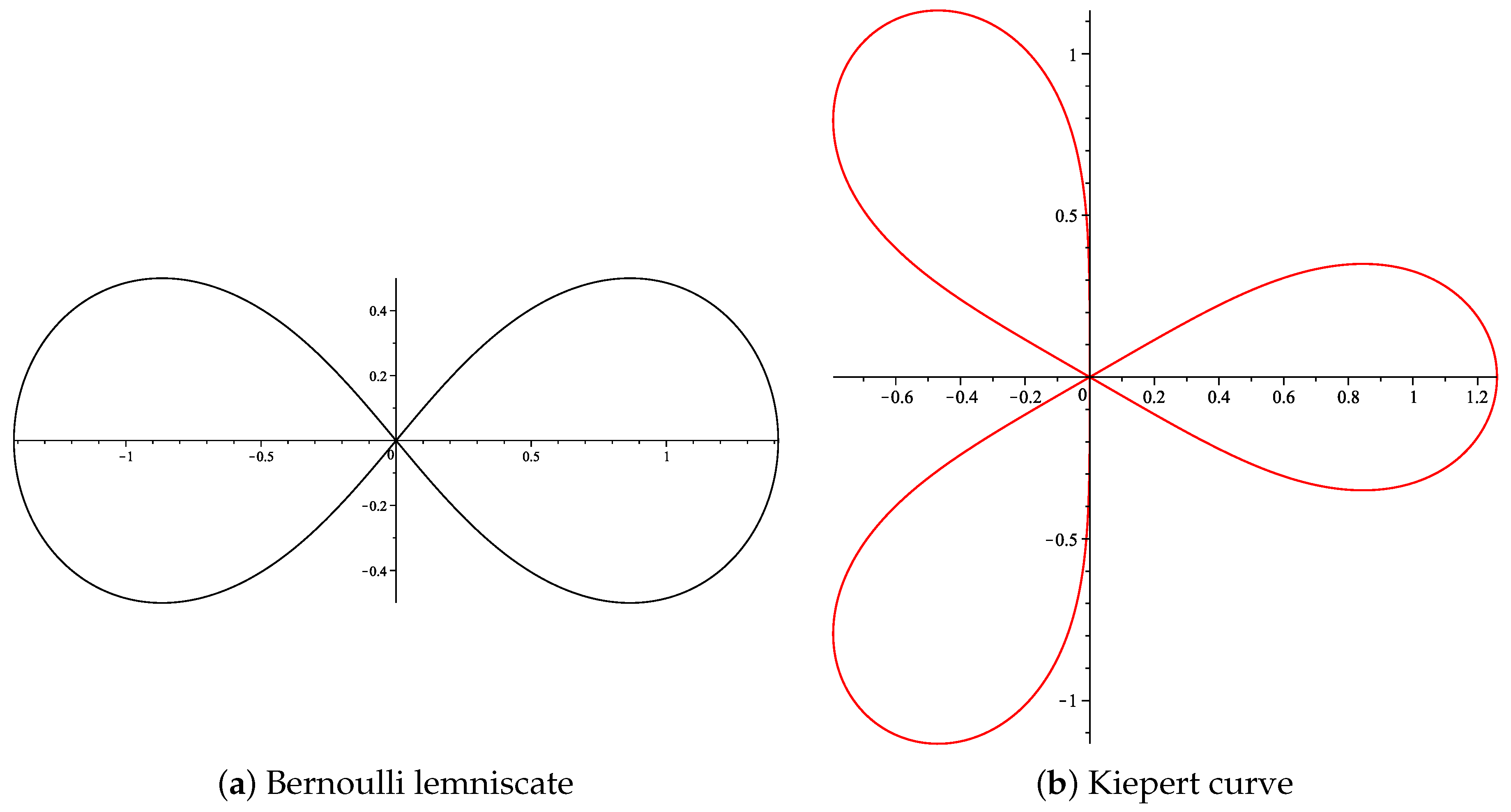
For $n=2$, the curve $P_2$ is the lemniscate of Bernoulli (see Figure 2a). For $n=3$, we obtain the Kiepert curve (see Figure 2b). In general, the curve $P_n$ defined by (13) is called a sinusoidal spiral or a lemniscate with n poles (see [42,43]). These algebraic curves having the polar equation $r^n=a^{n}cos\left(n\theta \right)$ ($n\in \mathbb{Q}$) were studied for the first time by Maclaurin in 1718.

The equation $|z^n-1|=1$ can be written in the equivalent form:

$$\left|z-{\omega }_n^0\right|·\left|z-{\omega }_n^1\right|·\dots ·\left|z-{\omega }_n^{n-1}\right|=1.$$

Therefore, if $A_0\left({\omega }_n^0\right),\dots A_{n-1}\left({\omega }_n^{n-1}\right)$ are the vertices of the regular polygon formed by the complex roots of unity, then $P_n$ is the set of all the points $M\left(z\right)$ that satisfy

$$M{A}_0·M{A}_1·\dots ·M{A}_{n-1}=1.$$

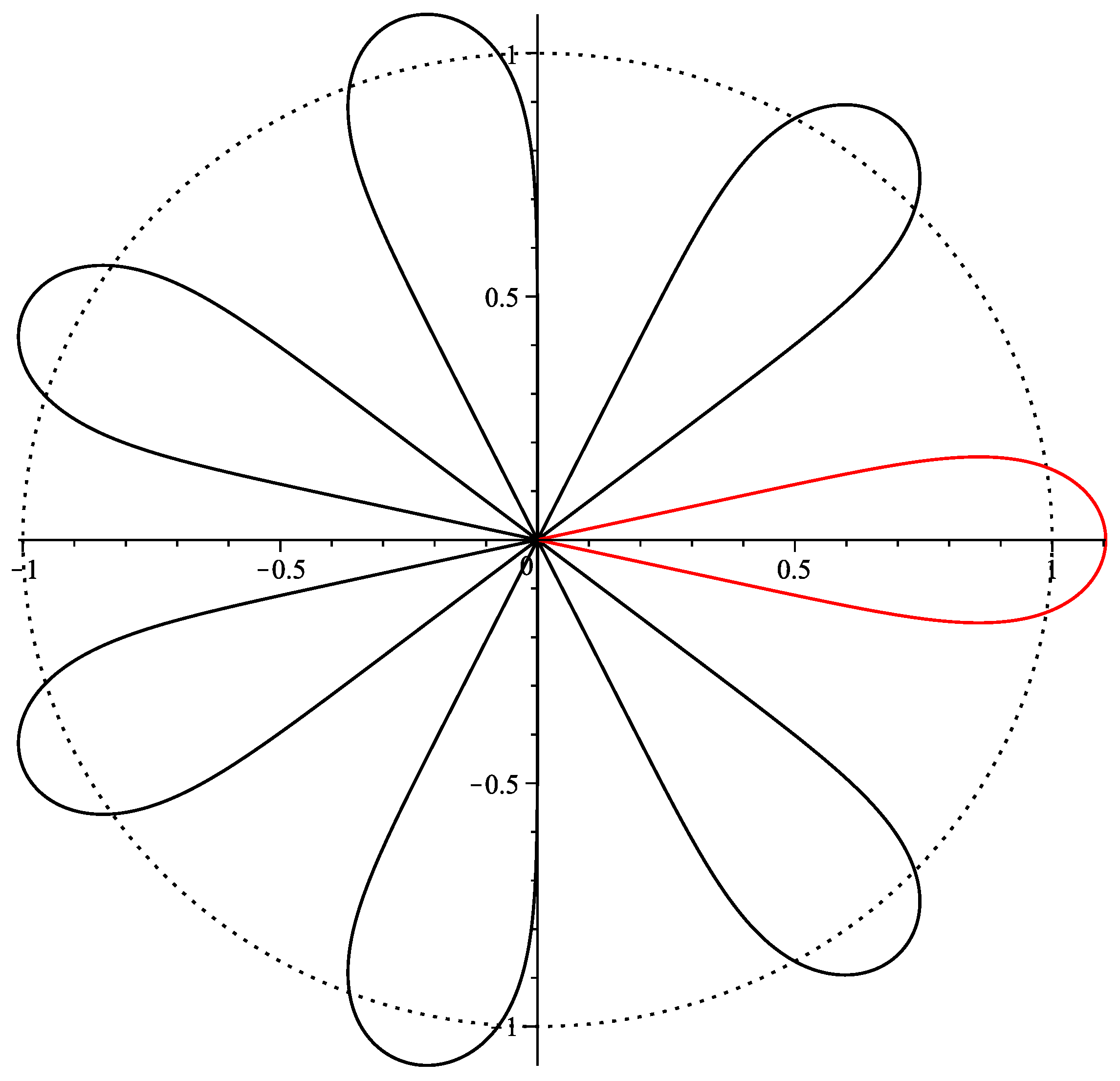
As can be easily noticed, a lemniscate with n poles is composed of n identical “petals” obtained by rotating the base pattern $P_n^0$ about the origin with angle $\frac{2j\pi }{n}$, $j=1,2,\dots ,n-1$ (see Figure 3):

$$P_n^j:z=\sqrt[n]{2cosn\theta }·e^{i\theta }·{\omega }_n^j,\theta \in \left[-\frac{\pi }{2n},\frac{\pi }{2n}\right],j=0,1,\dots ,n-1.$$

The “length” of each petal (the distance from the origin to the most distant point) is equal to $\sqrt[n]{2}$.

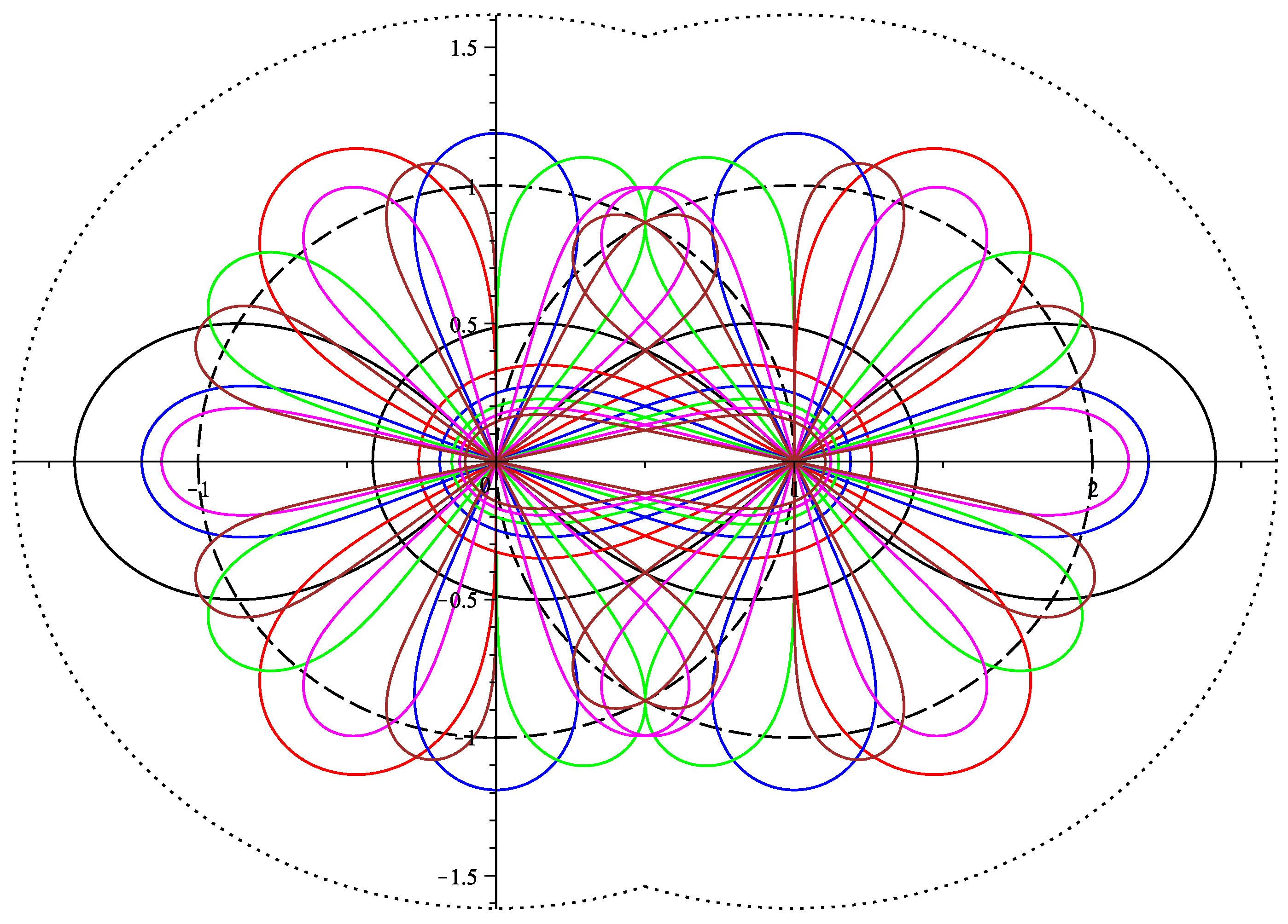
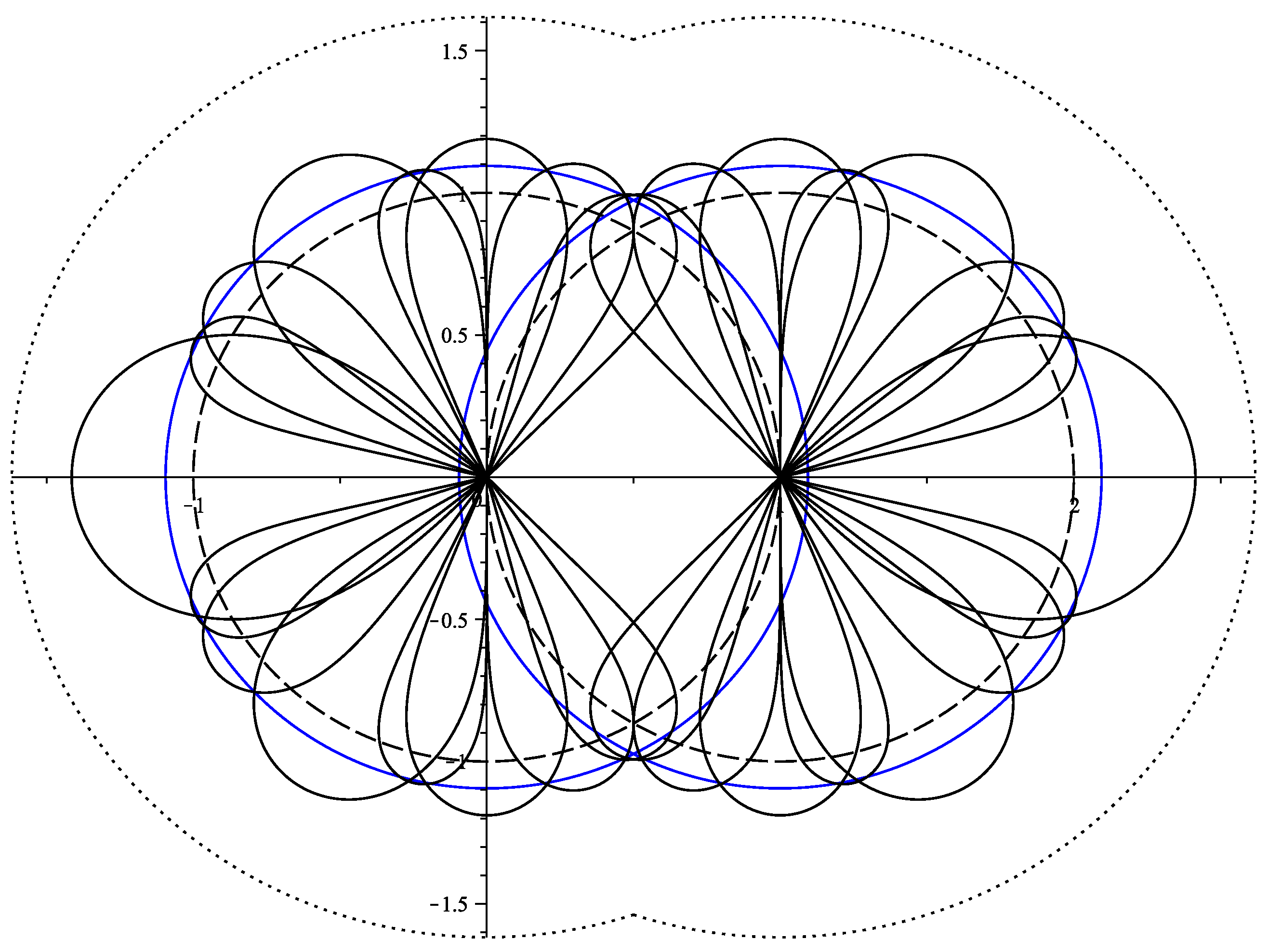
We present ${\mathcal{P}}_n$ and $1-{\mathcal{P}}_n$ for $n=2,\dots ,7$ in Figure 4 (exterior dot circles are centered at 0 and 1, respectively, and have the radius $\varphi$).

Obviously, the “petals” contained in the disks ${\mathcal{D}}_0\left(1\right)$ (and ${\mathcal{D}}_1\left(1\right)$) or those included in other petals are not of interest. We shall prove that the “interesting petals” are only those presented in Figure 5. Thus, the next theorem shows that the infinite union ${\mathcal{L}}_2\cup {\mathcal{R}}_2$ can be written as a finite union.

Theorem 3.

With the notations above, we have:

$${\mathcal{L}}_2\cup {\mathcal{R}}_2=\underset{n=2}{\overset{7}{\cup }}\left({\mathcal{P}}_n\cup (1-{\mathcal{P}}_n)\right).$$

(14)

Proof. 

To find the largest radius $r>0$ such that

$${\mathcal{D}}_0\left(r\right)\subset \underset{n=2}{\overset{7}{\cup }}\left({\mathcal{P}}_n\cup (1-{\mathcal{P}}_n)\right),$$

we calculate the intersections (other than the origin) of the “interesting petals” (due to the symmetry with respect to x axis, we need to study only the points above it). We present the results in

Table 1. Points of intersection of the “interesting petals”.

$\mathit{z}={\mathit{P}}_{{\mathit{n}}_1}^{{\mathit{j}}_1}\cap {\mathit{P}}_{{\mathit{n}}_2}^{{\mathit{j}}_2}$	$\left|\mathit{z}\right|$
$P_2^1\cap P_7^3$	$1.1038$
$P_7^3\cap P_5^2$	$1.0954$
$P_5^2\cap P_3^1$	$\mathbf{1}.\mathbf{0945}$
$P_3^1\cap P_7^2$	$1.1025$
$P_7^2\cap P_4^1$	$1.0990$
$P_4^1\cap P_5^1$	$1.1001$
$P_5^1\cap P_6^1$	$1.0993$

.

It follows that the largest disk contained in $\underset{n=2}{\overset{7}{\cup }}\left({\mathcal{P}}_n\cup (1-{\mathcal{P}}_n)\right)$ has the radius $r=1.0945>\sqrt[8]{2}$, which means that

$${\mathcal{P}}_m\cup (1-{\mathcal{P}}_m)\subset {\mathcal{D}}_0\left(r\right)\cup {\mathcal{D}}_1\left(r\right)\subset \underset{n=2}{\overset{7}{\cup }}\left({\mathcal{P}}_n\cup (1-{\mathcal{P}}_n)\right)$$

for every $m\ge 8$ and the theorem is proved. □

Figure 5 presents the set ${\mathcal{L}}_2\cup {\mathcal{R}}_2$ (only the significant petals are drawn). The blue circles are the circles of radius $1.0945$ centered at 0 and at 1.

Since ${\mathcal{L}}_2\cup {\mathcal{R}}_2$ is a finite union of “petals”, it follows that ${\mathcal{L}}_3\cup {\mathcal{R}}_3$ can be also written as a finite union as

$${\mathcal{L}}_3\cup {\mathcal{R}}_3=\underset{n=2}{\overset{7}{\cup }}\left({\phi }_n^{-1}\left({\mathcal{R}}_2\right)\cup 1-{\phi }_n^{-1}\left({\mathcal{R}}_2\right)\right),$$

and generally,

$${\mathcal{L}}_{k+1}\cup {\mathcal{R}}_{k+1}=\underset{n=2}{\overset{7}{\cup }}\left({\phi }_n^{-1}\left({\mathcal{R}}_k\right)\cup 1-{\phi }_n^{-1}\left({\mathcal{R}}_k\right)\right).$$

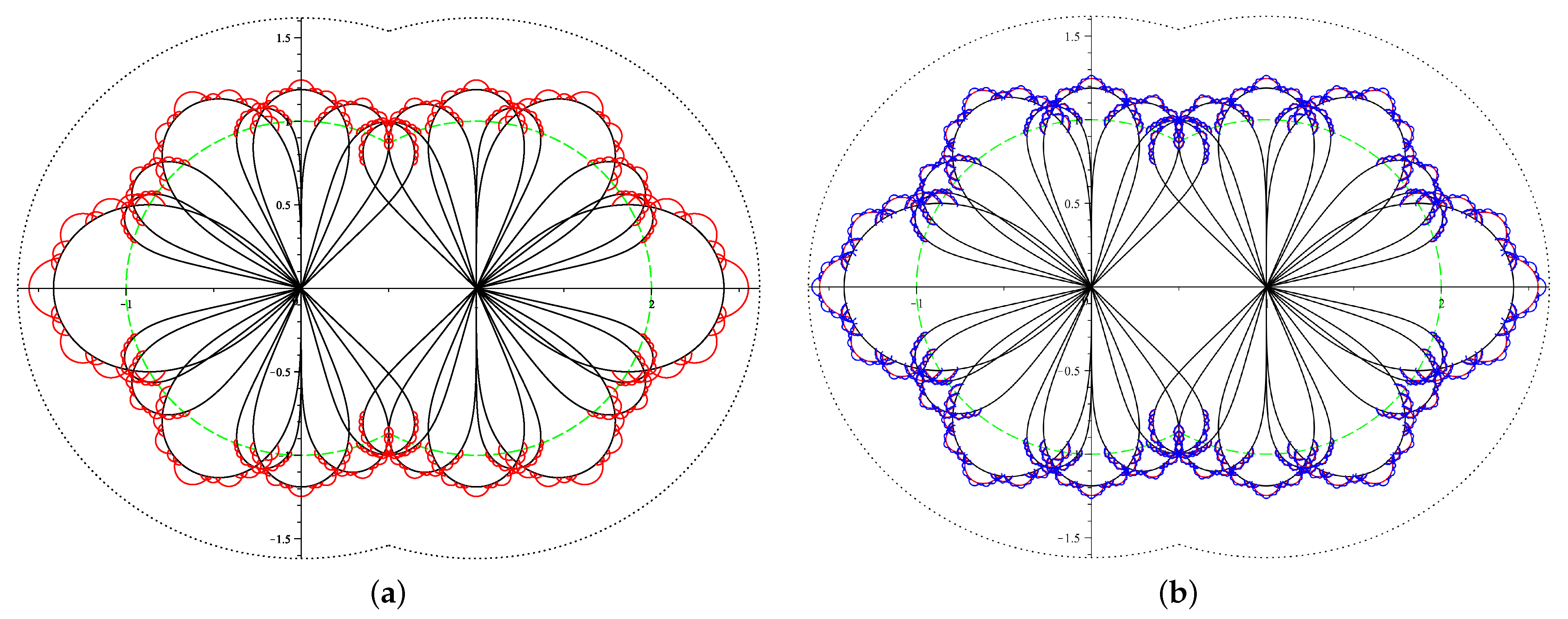
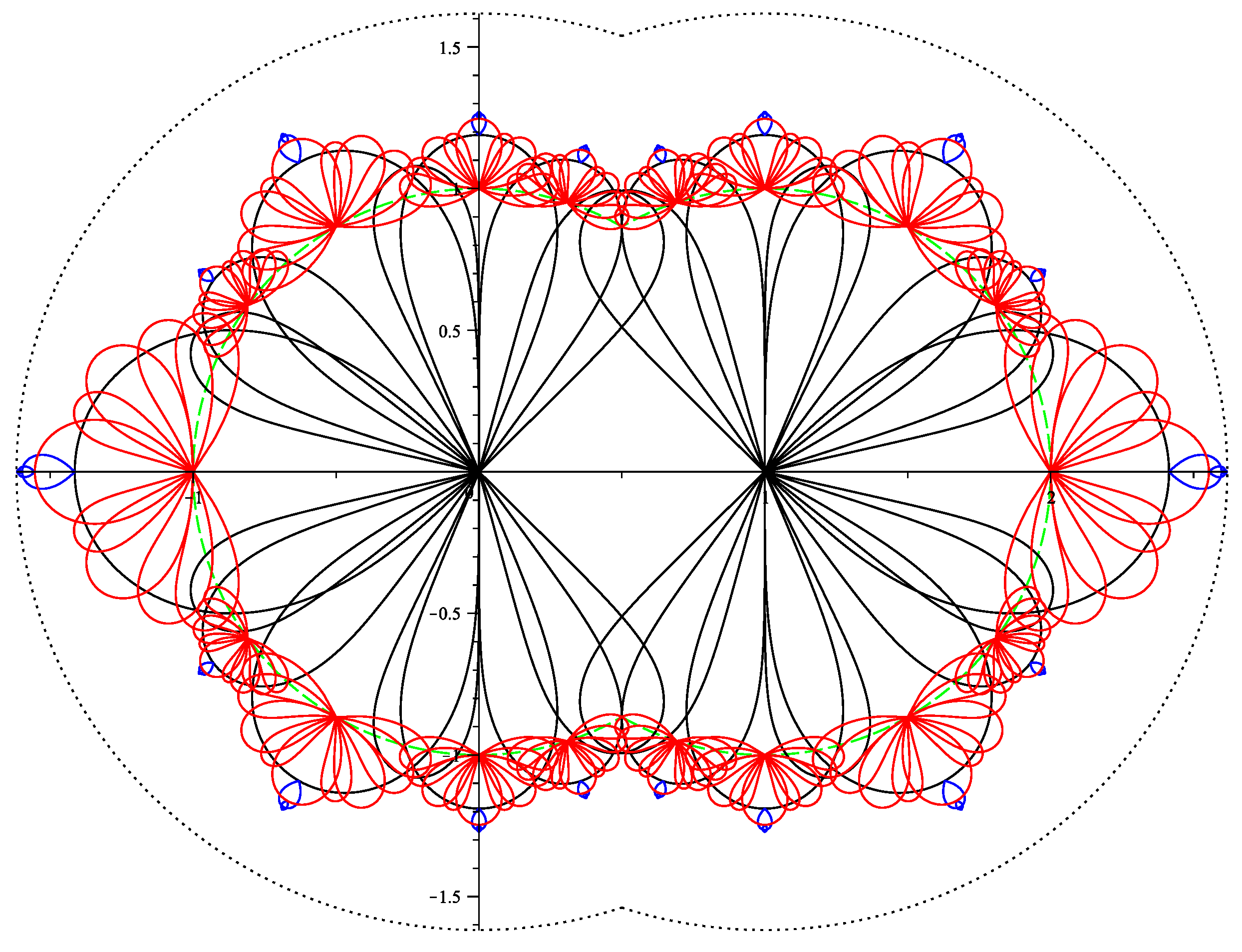
The sets ${\mathcal{L}}_3\cup {\mathcal{R}}_3$ and ${\mathcal{L}}_4\cup {\mathcal{R}}_4$ are presented in Figure 6: the boundary of ${\mathcal{L}}_3\cup {\mathcal{R}}_3$ is given by the red curves in Figure 6a, while the the boundary of ${\mathcal{L}}_4\cup {\mathcal{R}}_4$ is formed by the blue curves in Figure 6b. By comparing the two images in Figure 6, it becomes apparent that as k increases, the newly acquired domain $({\mathcal{L}}_{k+1}\cup {\mathcal{R}}_{k+1})\setminus ({\mathcal{L}}_k\cup {\mathcal{R}}_k)$ becomes progressively less significant, compared to the time required for calculations, which increases exponentially (representing the primary technical difficulty). Therefore, we let ${\mathcal{L}}_4\cup {\mathcal{R}}_4$ be an approximation of $\mathcal{S}$ and try to find (in the next section) some limit points.

5. Limit Points

As mentioned above, the difference between ${\mathcal{L}}_k\cup {\mathcal{R}}_k$ and ${\mathcal{L}}_{k+1}\cup {\mathcal{R}}_{k+1}$ tends to vanish as k increases. Although we cannot tell the exact expression of the boundary of $\overline{\mathcal{S}}$, we can find some limit points (belonging to the boundary of $\overline{\mathcal{S}}$).

First of all, we shall prove that the two limit points on the real axis are $-\varphi$ and $1+\varphi$.

The leftmost limit point is the limit of the sequence $\left\{x_n\right\}$ defined by the recurrence relationship

$$x_{n+1}={\psi }_2^{1}g\left(x_n\right)=-\sqrt{1-x_n}$$

(15)

for every $n\ge 1$, and $x_1=-1={\psi }_2^{1}g\left(0\right)$.

It can be easily proved that the sequence $\left\{x_n\right\}$ is monotonically decreasing and bounded; hence, it is convergent. Its limit ${\displaystyle \xi =\underset{n\to \infty }{lim}{x}_n}$ is the negative root of the equation

$${\xi }^2+\xi -1=0,$$

(16)

so $\xi =-\frac{1+\sqrt{5}}{2}=-\varphi$. Obviously, the rightmost limit point is $1-\xi =1+\varphi ={\varphi }^2$.

The limit points in the directions $argz=\frac{2\pi }{3}$ and $argz=\frac{4\pi }{3}$, respectively, are the limits of the sequences

$$\begin{array}{cc}\hfill y_n& ={\psi }_3^{1}g\underset{n}{\underbrace{{\psi }_2^{1}g{\psi }_2^{1}g\dots {\psi }_2^{1}g}}\left(0\right)={\psi }_3^{1}g\left(x_n\right),\hfill \\ \hfill z_n& ={\psi }_3^{2}g\underset{n}{\underbrace{{\psi }_2^{1}g{\psi }_2^{1}g\dots {\psi }_2^{1}g}}\left(0\right)={\psi }_3^{2}g\left(x_n\right),\hfill \end{array}$$

hence, we obtain another four limit points:

$$\begin{array}{cc}\hfill \underset{n\to \infty }{lim}{y}_n={\psi }_3^1(1+\varphi )={\varphi }^{\frac{2}{3}}exp\left(i\frac{2\pi }{3}\right)& \mathrm{and}1-{\varphi }^{\frac{2}{3}}exp\left(i\frac{2\pi }{3}\right),\hfill \\ \hfill \underset{n\to \infty }{lim}{z}_n={\psi }_3^2(1+\varphi )={\varphi }^{\frac{2}{3}}exp\left(i\frac{4\pi }{3}\right)& \mathrm{and}1-{\varphi }^{\frac{2}{3}}exp\left(i\frac{4\pi }{3}\right).\hfill \end{array}$$

Similarly, the limit points on the imaginary axis (in the directions $argz=\frac{\pi }{2}$ and $argz=\frac{3\pi }{2}$ respectively), together with their symmetrics w.r.t $\frac{1}{2}$ are given by:

$$\begin{array}{cc}\hfill \underset{n\to \infty }{lim}{\psi }_4^{1}g\left(x_n\right)={\psi }_4^1(1+\varphi )=i\sqrt{\varphi },& \mathrm{and}1-i\sqrt{\varphi }\hfill \\ \hfill \underset{n\to \infty }{lim}{\psi }_4^{3}g\left(x_n\right)={\psi }_4^1(1+\varphi )=-i\sqrt{\varphi },& \mathrm{and}1+i\sqrt{\varphi }.\hfill \end{array}$$

Finally, by considering the directions $argz=\frac{2\pi }{5},\frac{4\pi }{5},\frac{6\pi }{5},\frac{8\pi }{5}$, we find another 8 limit points:

$$\begin{array}{cc}\hfill \underset{n\to \infty }{lim}{\psi }_5^{1}g\left(x_n\right)={\psi }_5^1(1+\varphi )={\varphi }^{\frac{2}{5}}exp\left(i\frac{2\pi }{5}\right)& \mathrm{and}1-{\varphi }^{\frac{2}{5}}exp\left(i\frac{2\pi }{5}\right)\hfill \\ \hfill \underset{n\to \infty }{lim}{\psi }_5^{2}g\left(x_n\right)={\psi }_5^2(1+\varphi )={\varphi }^{\frac{2}{5}}exp\left(i\frac{4\pi }{5}\right)& \mathrm{and}1-{\varphi }^{\frac{2}{5}}exp\left(i\frac{4\pi }{5}\right)\hfill \\ \hfill \underset{n\to \infty }{lim}{\psi }_5^{3}g\left(x_n\right)={\psi }_5^3(1+\varphi )={\varphi }^{\frac{2}{5}}exp\left(i\frac{6\pi }{5}\right)& \mathrm{and}1-{\varphi }^{\frac{2}{5}}exp\left(i\frac{6\pi }{5}\right)\hfill \\ \hfill \underset{n\to \infty }{lim}{\psi }_5^{4}g\left(x_n\right)={\psi }_5^4(1+\varphi )={\varphi }^{\frac{2}{5}}exp\left(i\frac{8\pi }{5}\right)& \mathrm{and}1-{\varphi }^{\frac{2}{5}}exp\left(i\frac{8\pi }{5}\right)\hfill \end{array}$$

All of these limit points (together with the set ${\mathcal{L}}_3\cup {\mathcal{R}}_3$) are presented in Figure 7. For any $n\ge 6$ and $j=1,\dots ,n-1$, the points ${\psi }_n^j(1+\varphi )$ are not limit points because they are contained into ${\mathcal{L}}_n\cup {\mathcal{R}}_n$.

6. Discussion and Conclusions

The paper studies the set of roots of the family of polynomials obtained by composing $g\left(x\right)=1-x$ with polynomials of the type ${\phi }_n\left(x\right)=x^n$. The reliability polynomials of the networks created by series-parallel compositions belong to this family. We prove that the set of roots is bounded by the two circles of radius $\varphi$ centered at 0 and at 1.

Brown and deGagné have proved in [21] that the closure of two-terminal reliability roots contains the closed unit disks centered at 0 and at 1. We also study the closure of the set of roots of the family of polynomials considered and prove that it includes not only these two disks but also the domain bounded by the lemniscates with n poles, $\left|z^n-1\right|\le 1$ and $\left|{(1-z)}^n-1\right|\le 1$. We proved that the two disks completely covered by these sinusoidal spirals have a radius slightly greater than 1.

Some interesting open problems arise naturally:

• What is the maximum radius of the two disks contained into the closure of the set of roots?
• How can one find other limit points, apart from the ones presented in the last section of the paper?
• The real roots are proved to be in $(-\varphi ,0]\cup [1,1+\varphi )$, and the points $-\varphi$ and $1+\varphi$ are proved to be limit points. Is the set of real roots dense in $[-\varphi ,0]\cup [1,1+\varphi ]$?

References

- Cauchy, A.L. Exercises de Mathématique; Année 4. De Bure Frères: Paris, France, 1829. [Google Scholar]
- Gardner, R.; Govil, N.K. The Eneström–Kakeya Theorem and some of its generalizations. In Current Topics in Pure and Computational Complex Analysis; Joshi, S., Dorff, M., Lahiri, I., Eds.; Springer: New Delhi, India, 2014; pp. 171–200. [Google Scholar]
- Marden, M. Geometry of Polynomials, 2nd ed.; American Mathematical Society: Providence, RI, USA, 1966. [Google Scholar]
- Anderson, N.; Saff, E.B.; Varga, R.S. On the Enestróm-Kakeya theorem and its sharpness. Linear Algebra Appl. 1979, 28, 5–16. [Google Scholar] [CrossRef]
- Rahman, Q.I.; Schemeisser, G. Analytic Theory of Polynomials; London Mathematical Society Monographs (New Series 26); Oxford University Press: Oxford, UK, 2002. [Google Scholar]
- Moore, E.F.; Shannon, C.E. Reliable circuits using less reliable relays—Part I. J. Frankl. Inst. 1956, 262, 191–208. [Google Scholar] [CrossRef]
- Colbourn, C.J. The Combinatorics of Network Reliability; Oxford University Press: New York, NY, USA, 1987. [Google Scholar]
- Colbourn, C.J. Combinatorial aspects of network reliability. Ann. Oper. Res. 1991, 33, 1–15. [Google Scholar] [CrossRef]
- Valiant, C. The complexity of enumeration and reliability problems. SIAM J. Comput. 1979, 8, 410–421. [Google Scholar] [CrossRef]
- Beiu, V.; Drăgoi, V.F.; Beiu, R.M. Why reliability for computing needs rethinking. In Proceedings of the 2020 International Conference on Rebooting Computing (ICRC), Atlanta, GA, USA, 1–3 December 2020; IEEE: Piscataway, NJ, USA, 2020; pp. 16–25. [Google Scholar]
- Cristescu, G.; Drăgoi, V.F. Efficient approximation of two-terminal networks reliability polynomials using cubic splines. IEEE Trans. Reliab. 2021, 70, 1193–1203. [Google Scholar] [CrossRef]
- Jianu, M.; Ciuiu, D.; Dăuş, L.; Jianu, M. Markov chain method for computing the reliability of hammock networks. Probab. Eng. Inf. Sci. 2022, 36, 276–293. [Google Scholar] [CrossRef]
- Cowell, S.R.; Hoară, S.; Beiu, V. Experimenting with beta distributions for approximating hammocks’ reliability. In Intelligent Methods in Computing, Communications and Control, Proceedings of the 8th International Conference on Computers Communications and Control (ICCCC 2020), Oradea, Romania, 11–15 May 2020; Springer: Cham, Switzerland, 2021; pp. 70–81. [Google Scholar]
- Jianu, M.; Dăuş, L.; Hoară, S.H.; Beiu, V. Using Delta-Wye transformations for estimating networks’ reliability. In Intelligent Methods Systems and Applications in Computing, Communications and Control, Proceedings of the 9th International Conference on Computers Communications and Control (ICCCC 2022), Oradea, Romania, 16–20 May 2022; Springer: Cham, Switzerland, 2023; pp. 415–426. [Google Scholar]
- Dăuş, L.; Jianu, M. Full Hermite interpolation of the reliability of a hammock network. Appl. Anal. Discret. Math. 2020, 14, 198–220. [Google Scholar] [CrossRef]
- Cristescu, G.; Drăgoi, V.F.; Hoară, S.H. Generalized convexity properties and shape-based approximation in networks reliability. Mathematics 2021, 9, 3182. [Google Scholar] [CrossRef]
- Dăuş, L.; Jianu, M. The shape of the reliability polynomial of a hammock network. In Intelligent Methods in Computing, Communications and Control, Proceedings of the 8th International Conference on Computers Communications and Control (ICCCC 2020), Oradea, Romania, 11–15 May 2020; Springer: Cham, Switzerland, 2021; pp. 93–105. [Google Scholar]
- Graves, C.; Milan, D. Reliability polynomials having arbitrarily many inflection points. Networks 2014, 64, 1–5. [Google Scholar] [CrossRef]
- Mol, L. On Connectedness and Graph Polynomials. Ph.D. Thesis, Dalhousie University, Halifax, NS, Canada, 2016. [Google Scholar]
- Brown, J.I.; Colbourn, C.J. Roots of the reliability polynomial. SIAM J. Discr. Math. 1992, 5, 571–585. [Google Scholar] [CrossRef]
- Brown, J.I.; DeGagné, C.D.C. Roots of two-terminal reliability polynomials. Networks 2021, 78, 153–163. [Google Scholar] [CrossRef]
- Dăuş, L.; Drăgoi, V.F.; Jianu, M.; Bucerzan, D.; Beiu, V. On the roots of certain reliability polynomials. In Intelligent Methods Systems and Applications in Computing, Communications and Control, Proceedings of the 9th International Conference on Computers Communications and Control (ICCCC 2022), Oradea, Romania, 16–20 May 2022; Springer: Cham, Switzerland, 2023; pp. 401–414. [Google Scholar]
- DeGagné, C.D.C. Network Reliability, Simplicial Complexes, and Polynomial Roots. Ph.D. Thesis, Dalhousie University, Halifax, NS, Canada, 2020. [Google Scholar]
- Royle, G.; Sokal, A.D. The Brown–Colbourn conjecture on zeros of reliability polynomials is false. J. Comb. Theory 2004, 91, 345–360. [Google Scholar] [CrossRef]
- Birkhoff, G.D. A determinantal formula for the number of ways of coloring a map. Ann. Math. 1912, 14, 42–46. [Google Scholar] [CrossRef]
- Cameron, P.J.; Morgan, K. Algebraic properties of chromatic roots. Electron. J. Comb. 2017, 24, 1–21. [Google Scholar] [CrossRef] [PubMed]
- Jackson, B. A zero-free interval for chromatic polynomials of graphs. Comb. Probab. Comput. 1993, 2, 325–336. [Google Scholar] [CrossRef]
- Sokal, A.D. Chromatic roots are dense in the whole complex plane. Comb. Probab. Comput. 2004, 13, 221–261. [Google Scholar] [CrossRef]
- Thomassen, C. The zero-free intervals for chromatic polynomials of graphs. Comb. Probab. Comput. 1997, 6, 497–506. [Google Scholar] [CrossRef]
- Gutman, I.; Harary, F. Generalizations of the matching polynomial. Util. Math. 1983, 24, 97–106. [Google Scholar]
- Brown, J.I.; Hickman, C.A.; Nowakowski, R.J. On the location of roots of independence polynomials. J. Algebr. Comb. 2004, 19, 273–282. [Google Scholar] [CrossRef]
- Brown, J.I.; Cameron, B. A note on purely imaginary independence roots. Discrete Math. 2020, 343, 112113. [Google Scholar] [CrossRef]
- Arocha, J.L.; Llano, B. Mean value for the matching and dominating polynomial. Discuss. Math. Graph Theory 2000, 20, 57–69. [Google Scholar] [CrossRef]
- Beaton, I.; Brown, J.I. On the real roots of domination polynomials. Contrib. Discret. Math. 2021, 16, 175–182. [Google Scholar]
- Beaton, I.; Brown, J.I.; Cox, D. Optimal domination polynomials. Graph. Combinator. 2020, 36, 1477–1487. [Google Scholar] [CrossRef]
- Beaton, I.; Brown, J.I. On the unimodality of domination polynomials. Graphs Comb. 2022, 38, 90. [Google Scholar] [CrossRef]
- Brown, J.I.; Tufts, J. On the roots of domination polynomials. Graphs Comb. 2014, 30, 527–547. [Google Scholar] [CrossRef]
- Drăgoi, V.F.; Beiu, V. Fast reliability ranking of matchstick minimal networks. Networks 2022, 79, 479–500. [Google Scholar] [CrossRef]
- Drăgoi, V.F.; Cowell, S.R.; Beiu, V. Ordering series and parallel compositions. In Proceedings of the 2018 IEEE 18th International Conference on Nanotechnology (IEEE-NANO), Cork, Ireland, 23–26 July 2018; IEEE: Piscataway, NJ, USA, 2019; pp. 1–4. [Google Scholar]
- Drăgoi, V.F.; Cowell, S.R.; Beiu, V.; Hoară, S.; Gaspar, P. How reliable are compositions of series and parallel networks compared with hammocks? Int. J. Comput. Commun. Control 2018, 13, 772–791. [Google Scholar] [CrossRef]
- Beardon, A. Iteration of Rational Functions; Springer: New York, NY, USA, 1991. [Google Scholar]
- Lawrence, J.D. A Catalog of Special Plane Curves; Dover: New York, NY, USA, 1972; p. 184. [Google Scholar]
- Lockwood, E.H. A Book of Curves; Cambridge University Press: London, UK, 1961; p. 175. [Google Scholar]
Figure 1.
Bounds of the set of roots .
Figure 2.
The curves for and .
Figure 3.
Lemniscate with seven poles. The red-colored curve is .
Figure 4.
Lemniscates with poles, centered at 0 and at 1.
Figure 5.
The set . The blue circles have the radius 1.0945.
Figure 6.
(a) The set . (b) The set .