Article

Tool Degradation Prediction Based on Semimartingale Approximation of Linear Fractional Alpha-Stable Motion and Multi-Feature Fusion

1
School of Electronic & Electrical Engineering, Shanghai University of Engineering Science, Shanghai 201620, China
2
College of Information Management, Minnan University of Science and Technology, Quanzhou 362700, China
3
Department of Computer, Control and Management Engineering, University of Rome La Sapienza, Via Ariosto 25, 00185 Roma, Italy
4
Department of Medical Physics and Informatics, Bashkir State Medical University, Lenina 3, 450008 Ufa, Russia
5
Department of Industrial Engineering, University of Salerno, Via Giovanni Paolo II 132, 84084 Fisciano, Italy
*
Author to whom correspondence should be addressed.
Fractal Fract. 2023, 7(4), 325; https://doi.org/10.3390/fractalfract7040325
Submission received: 20 March 2023 / Revised: 7 April 2023 / Accepted: 9 April 2023 / Published: 12 April 2023
(This article belongs to the Special Issue New Trends in Fractional Stochastic Processes)

Abstract

:
Tool wear will reduce workpieces’ quality and accuracy. In this paper, the vibration signals of the milling process were analyzed, and it was found that historical fluctuations still have an impact on the existing state. First of all, the linear fractional alpha-stable motion (LFSM) was investigated, along with a differential iterative model with it as the noise term is constructed according to the fractional-order Ito formula; the general solution of this model is derived by semimartingale approximation. After that, for the chaotic features of the vibration signal, the time-frequency domain characteristics were extracted using principal component analysis (PCA), and the relationship between the variation of the generalized Hurst exponent and tool wear was established using multifractal detrended fluctuation analysis (MDFA). Then, the maximum prediction length was obtained by the maximum Lyapunov exponent (MLE), which allows for analysis of the vibration signal. Finally, tool condition diagnosis was carried out by the evolving connectionist system (ECoS). The results show that the LFSM iterative model with semimartingale approximation combined with PCA and MDFA are effective for the prediction of vibration trends and tool condition. Further, the monitoring of tool condition using ECoS is also effective.

1. Introduction

In this paper, the aim is to use the LRD of data to develop a differential iterative model based on LFSM, predicting the trend of tool’s vibration by the model’s general solution, which is derived by semimartingale approximation. The monitoring of tool wear status is subsequently implemented via ECoS. In this section, the background, literature review, formulation of the problem, research in this paper, and the organization of this paper are provided.

1.1. Background

The tool, as a crucial basic component of the milling machine, is one of the most important components in ensuring machining quality and lowering machining costs, but it is also the most susceptible component [1]. According to research, tool wear is the most common cause of milling process failures. As a result, the tool’s evaluation and prediction is important. In this paper, the tool’s vibration signal data is employed for prediction.

1.2. Literature Review

The tool degradation state can be divided into direct measurement methods and indirect measurement methods. The direct methods refer to the measurement of parameters related to the tool’s volume, mainly optical measurements and computer image processing [2]. Zhu et al. [3] proposed a tool wear surface area monitoring method, which decomposed the original micro-milling tool image into the target tool image, background image, and noise image. This method uses an area growth algorithm based on morphological component analysis to detect defects and extract the wear area of the target tool image. Szydowski et al. [4] proposed a wavelet transform-based image reconstruction method to overcome the scatter phenomenon in tool imaging and to evaluate tool wear using geometric information properties. This type of method is not applicable to industrial fields because it requires interrupting the machining process while monitoring tool wear status. It is difficult to achieve online real time work and the equipment is expensive. Therefore, indirect methods are the main research method of scholars.
Indirect methods usually refer to the vibration, cutting force, acoustic signals, and other data acquired by sensors. In this paper, we only investigate the relationship between the vibration signal and tool degradation trend. Vibration has a strong connection with the cutting force and has its own dynamic characteristics. As the wear of the tool increases or the tool breaks, the frictional state of the contact part between the tool and the workpiece changes, causing fluctuations in the signal of the cutting forces, which leads to variations in frequency and amplitude of vibration. The vibration signal is highly sensitive to tool wear and damage. Choudhury et al. [5] developed mathematical models of wear and diffusion indices, wear coefficients, normal loads, and other factors for tool wear prediction. Salgado et al. [6] used singular spectrum analysis (the method uses PCA to decompose the time series into multiple independent sets), extracted information related to the tool state, and then predicted the tool wear trend by constructing a neural network. Elangovan et al. [7] used a data mining approach to predict degradation features in the vibration signal that were extracted by using PCA, then compared with PCA feature transformation and decision tree feature transformation to improve the robustness of the classifier. Gong et al. [8] presented a method to decompose the vibration signal using FFT to obtain the damping ratio and used it to predict the vibration trend of the tool.
Several common techniques are available. Refs. [9,10] created physics-based variance analysis for tool wear prediction and regression analysis of cutting processes. Ref. [11] developed a tool wear prediction method using artificial neural networks. Ref. [12] also developed a support vector machine prediction method [11,12], which is also an indirect method. Due to the fact that they are trained on historical data samples, these models inherently acquire the characteristics of the training samples by default. They ignore the long-range dependence (LRD) and self-similarity that the time series data has. The LFSM iterative prediction model proposed in this paper adopts these shortcomings and thus is more accurate than the above models and can be used with ECoS for more accurate tool wear detection.
The concept of fractal geometry was first introduced by the mathematician B.B. Mandelbrot in 1975 [13,14], but earlier work can be traced back to the nineteenth century. In 1875, K. Weierestrass constructed functions that are everywhere continuous but everywhere infinitesimal. G. Cantor constructed stop-trivial Cantor sets with many singular properties in 1883; in 1890, G. Peano constructed curves that fill spaces, and in 1904, H. Koch designed a class of curves resembling snowflakes and the edges of islands. In 1915, W. Sierpinski designed geometric maps, such as carpets and sponges. They all have self-similarity, i.e., they consist of parts that are in some way similar to the whole. In 1978, Sayles and Thomas [15] published a paper in Nature about the thickness variation of rough surface morphology as a non-smooth stochastic process. Fractal parameters can be used to quantitatively characterize rough surfaces. The feature is scale-independent and it provides information on the full range of surface morphologies present on fractal surfaces at all scales [15]. Thomas [15] and Majumdar [16] were the first to apply fractal theory to the study of rough surfaces, using the fractal dimension D to quantitatively characterize rough surfaces. Inspired by the above experts, in this paper, we used fractal theory to research the wear condition of rear tool face. By analyzing the tool vibration signal, it is concluded that it has fractal characteristics and that the relationship between D and the Hurst index has been proven.
In 1974, applied chemist K. B. ldham and mathematician J. Spanier collaborated to publish the first monograph on fractional-order calculus [17]: Fractional Calculus: Theory and Applications, Differentiation, and Integration to Arbitrary Order. It is the first detailed explanation of the basic theory of fractional-order calculus and its applications. Fractional-order control was first introduced by Tustin in a paper on multi-objective position control, and some other studies were summarized by S. Manabe in the 1960s [18]. In 1993, French scholar A. Oustaloup designed the first generation of fractional-order from the view of fractional-order robust CRONE (robust control of non-integer order) controllers and was the first to successfully apply them [19]. In 1999, Slovakian scholar I. Podlubny published a book about fractional-order differential equations [20], which introduced the calculation of fractional-order calculus and the solution of fractional-order differential equations, providing a fractional-order differential and fractional-order integral. It also introduces some common engineering tools, such as Laplace and Fourier, which transform into fractional-order control systems, providing a physical explanation of fractional-order differentiation and fractional-order integration, making a fundamental contribution to the development of fractional-order control theory.

1.3. Formulation of the Problem

The vibration signal has LRD, and the prediction accuracy of current methods is not sufficient. There are difficulties in determining the maximum prediction length of a chaotic signal. It is neither a Markov process nor a semimartingale, so the differential iterative model based on LFSM does not satisfy the conditions for the solutions of the Ito formula. The vibration signal contains many time-frequency domain factors, which require simpler operations in the case of large amounts of data. Finally, signs need to be found that can reflect the state of tool wear. Therefore, to achieve tool wear detection, firstly, the LFSM differential iterative model must be built and solved. Secondly, the degradation characteristics and maximum prediction length must be determined. Finally, the signs of tool wear states must be analyzed.

1.4. Researches in This Paper

In recent years, it has been demonstrated that many stochastic sequences do not follow Markov processes not only during the most recent point of time, but can also influence future events earlier. This phenomenon is referred to as LRD. Studies in [21,22] demonstrate that LRD can provide better predictions than current techniques by taking into account both the past and future conditions. LFSM [23,24] is a stochastic process prediction approach where historical data must satisfy LRD. The most popular forecasting technique among those who use LRD properties is the fractional Brownian motion (fBm) [25,26]. The LRD characteristic of fBm is defined by just one parameter, H (Hurst index). The LRD properties of LFSM are established by two parameters, H and α, in contrast to fBm, where H specifies the global properties and α specifies the local properties. When α H > 1 , the LRD phenomenon occurs in LFSM [27,28]. This phenomenon allows LFSM to handle more complex situations than fBm and provides a more suitable description of LRD processes. As a result, we use an LFSM-based differential iterative prediction model for tool vibration signal prediction.
In this paper, an Ito integral [29,30] driven by LFSM with Riemann–Liouville type leads to construction of a differential iterative formula. Its relationship with noise is obtained from the fractional-order Taylor formula [31], and is generalized to the fractional-order Maruyama representation, constructing a semimartingale approximation for LFSM that converges consistently on L 2 Ω , resulting in the general solution for the differential iterative formula.
The small data method [32] is used to analyze MLE. By raising the time step of each iteration, the accuracy and speed of calculating are increased. This gives the maximum prediction length of the LFSM differential iterative model. In this paper, PCA is used to extract the main factors which influence the vibration trend in order to reduce the amount of calculation. Ten basic features based on time and frequency domain were selected: mean of absolute values, variance, kurtosis, margin factor, crest factor, impulse factor, waveform factor, vibration velocity energy, vibration intensity, and mean of power spectrum. The traditional dimensionless feature can accurately extract the weak degradation of the initial stage, but the extraction accuracy gradually decreases as degradation increases; the dimensional feature is highly influenced by energy and is insensitive to the weak trend of the initial degradation stage; the new dimensionless feature is insensitive to energy, however it can only properly extract the weak trend of the early deterioration stage. These variables may be related and have a clear impact on the outcome [33,34]. After forecasting the vibration trend, the MDFA algorithm is used to obtain the relationship between the generalized Hurst index and the wear state. The EClfoS system learned to enable earlier monitoring of tool wear.
This paper uses multi-sensor vertical mill monitoring data from the 2010 Prognostics and Health Management (PHM) Challenge for verification [35]. The prediction model in this paper is more flexible than the widely used fBm model and enables earlier prediction of vibration signals or wear states than existing methods. This paper uses an innovative method of constructing semimartingales to approximate the general solution, proving the uniqueness of the solution and reducing the difficulty of simulation. It is shown that the LFSM model can describe stochastic processes with LRD.

1.5. Advantages of the Paper

The methods presented in Section 1.2 mostly use historical data to train the model, so the predicted results present the characteristics of the training sample. The model in this paper takes full account of the LRD and self-similarity between historical and future data and can present longer and more accurate prediction distances. Finally, the existence and uniqueness of the model’s solution under research is proven by establishing the semimartingale, which in turn proves the validity of simulating random paths with this model. The model can be applied to many situations that require consideration of the LRD of data.

1.6. Organization of the Paper

This paper is organized as follows. In Section 2, the LFSM with LRD and self-similarity is researched and proved; Section 3 investigates the numerical simulation of LFSM, constructing a semimartingale with consistent convergence on L 2 Ω . Section 4 investigates the differential iterative model of LFSM, proves that the model has a unique solution by the semimartingale in Section 2, and estimates the LFSM model’s parameters; Section 5 presents PCA and MLE. Firstly, PCA is used to obtain the health factors, which mainly affect the degradation trend, and MLE is used to obtain the maximum predicted length; Section 6 describes the method for calculating the fractal dimension; Section 7 investigates the LFSM model to predict tool vibration data and compares it with some existing methods, which have a higher accuracy; Section 8 gives conclusions.

2. Linear Fractional Stable Motion in Alpha-Stable Case

2.1. Linear Alpha-Stable Motion

An alpha-stable motion is defined as follows [24,36]:
φ ϑ : α , β , μ , δ = E e j ϑ x = exp j μ ϑ δ ϑ α 1 j β ϑ ϑ tan π α 2 , α 1 exp j μ ϑ δ ϑ α 1 + j β ϑ ϑ 2 π ln ϑ , α = 1
where the index α 0,2 is the stability index and indicates the degree of local influence. The random sequence is skewed if the parameter β [ 1,1 ] is not satisfied by β = 0 , where a positive skewness is in the right tail and a negative skewness is in the left tail. The effects of α and β are shown in Figure 1. The parameter μ R controls the location property of the distribution. The parameter δ 0 indicates how discrete the distribution is from the mean. The effects of μ and δ are shown in Figure 2. Being X, the random variables that obey the Equation (1) as X ~ S α ( β , μ , δ ) .

2.2. A Type of LFSM

The LFSM is defined as follows [37]:
L H , α t = + { a [ t v + H 1 / α ( v ) + H 1 / α ] + b [ t v H 1 / α ( v ) H 1 / α ] } N d v
where a and b are real constants, and N R is an alpha-stable measure in the Lebesgue measure.
The incremental process is described below:
X H , α t = L H , α t + 1 L H , α t X H , α t = { a [ t + 1 s + H 1 / α s + H 1 / α ] + b [ t + 1 s H 1 / α s H 1 / α ] } ω α s
where ω α ( s ) is the Lévy white noise. X H , α ( t ) is known as the LFSM noise. LFSM is a self-similarity process where H 1 / α , and its incremental process, the noise X H , α ( t ) is a self-similarity process too. The proof of the self-similarity of LFSM is given below:
Define an integral kernel function,
f α , H a , b ; t , s = a [ t s + H 1 / α s + H 1 / α ] + b [ t + 1 s H 1 / α s H 1 / α ]
Define a function x α = x α , x 0 x α , x < 0 , then
c a H j = 1 d θ j f α , H a , b ; c t j + h , s f α , H a , b ; h , s α β s d s = j = 1 d θ j f α , H a , b ; t s , s f α , H a , b ; 0 , s α β ( c s + h ) d s
where θ , t , h R , c > 0 , d 1 , j = 1 , , d and β ( x ) is skewness intensity.
If H = 1 / α , the function f α , H a , b ; t , s becomes a constant; when H 1 / α , the function f α , H a , b ; t , s consistently describes the current state similarly to all past states. LFSM satisfies the definition of self-similarity property, X a t = a H X ( t ) , at H 1 / α .
LFSM has LRD only at α H > 1 [38]. It was notable that when α ( 0,1 ) , the model based on LFSM is not LRD. In order to describe the LRD data, α ( 1,2 ) is limited to ensure the reasonableness of the LFSM model for predictions. Additionally, it is required that 0.5 < H < 1 .

3. Numerical Simulation of LFSM and Approximation of Semimartingale

Using semimartingale to simplify Equation (2), the numerical simulation of LFSM is performed using the following two steps:
Step 1: The Lévy noise is convolved with the fractional-order integrator to obtain the fractional noise;
Step 2: The obtained fractional noise is integrated or accumulated to obtain the numerical expression of LFSM. Figure 3 depicts the generation process.
Therefore, the expression of the LFSM model simulation sequence can be obtained below:
L α , H t = 1 Γ ( a + 1 ) 0 t ( t s ) a d W = 1 Γ ( a + 1 ) 0 t ( t s ) a w ( s ) d s
where a = H 1 α , H ( 0,1 ) , α ( 0,2 ) , so a ( 0.5 , 0.5 ) , W indicates linear alpha-stable motion. Accordingly, the LFSM noise and LFSM can be simulated according to Equation (6) (see Figure 4).
In fractional stochastic calculus, we can use L t = 0 t ( t s ) a d W s instead of L α , H for the approximate calculation. Obviously, L α , H is not a semimartingale. L t = Γ ( a + 1 ) L α , H is also not a semimartingale.
To solve the fractional-order stochastic differential equations, we build a semimartingale L t ε that converges consistently with LFSM L t on the L 2 ( Ω ) area, as explained in Corollary 1 and 2.
Corollary 1.
L t ε = 0 t ( t s + ε ) a d W s
where a = H - 1 α , H 1 2 , 0 < H < 1, t 0 , for every ε > 0 , L t ε is a semimartingale.
Proof. 
Define a stochastic process Φ t ε that satisfies
Φ t ε = 0 t ( t s + ε ) a 1 d W u
Integrating Equation (8),
0 t Φ t ε d s = 0 t 0 s ( s u + ε ) a 1 d W u d s = 0 t u s ( s u + ε ) a 1 d s d W u = 1 a 0 t ( t u + ε ) a d W u ε a W t = 1 a L t ε ε a W t
Therefore,
L t ε = a 0 t Φ t ε d s + ε a W t
So, L t ε is a semimartingale. □
Corollary 2.
L t ε  converges uniformly to  L t  in  L 2 ( Ω )  when the case of  ε 0  and  t [ 0 , T ] .
Proof. 
According to the finite increment theorem
t s + ε a t s a a ε sup 0 γ 1 t s + γ ε a 1 = a ε t s a 1
According to the theory of isometry of Ito integrals
E L t ε L t 2 = E 0 t ( t s + ε ) a ( t s ) a d W s 2 = 0 t ( t s + ε ) a ( t s ) a 2 d s = 0 t ε ( t s + ε ) a ( t s ) a 2 d s + t ε t ( t s + ε ) a ( t s ) a 2 d s
According to the Equation (10), the Equation (12)’s left part:
0 t ε ( t s + ε ) a ( t s ) a 2 d s a 2 ε 2 0 t ε ( t s ) 2 a 2 d s
The Equation (12)’s right part:
t ε t ( t s + ε ) a ( t s ) a 2 d s a 2 ε 2 t ε t ( t s ) 2 a d s
According to Equations (13) and (14), we can get:
L t ε L t 2 a 2 ε 2 0 t ε t s 2 a 2 d s + a 2 ε 2 t ε t t s 2 a d s C ( a ) ε 1 + 2 a
We know that the Euclidean norm L t ε L t = ( E ( L t ε L t 2 ) ) 1 / 2 , so
L t ε L t 2 C ( a ) ε 1 + 2 a sup 0 t T
Corollary 2 is proved. □

4. Differential Iterative Model Based on LFSM

4.1. The Forecasting Model

The relationship between the degradation of the tool and the number of runs is described by the Black–Scholes formula for the stochastic process sequence X t , t > 0 . It is easy to derive a differential iterative formula based on linear alpha-stable motion, which can be expressed as follows:
d X t = μ X ( t ) d t + δ X ( t ) d L ( t )
where d X ( t ) is the increment of the stochastic process, μ is the drift function, δ is the diffusion function, μ and δ depict nonlinear degradation with power-law variation, X ( 0 ) is the initial state, and d L ( t ) denotes the increment of linear alpha-stable motion.
However, Equation (17) is only predicted favorably when it is satisfied that the degradation process has independent step increments. Obviously, it does not apply well to tool vibration with LRD. The LFSM is therefore introduced by modifying the diffusion term, and the results are shown below:
d X α , H t = μ X α , H t d t + δ X α , H t d L α , H ( t )
Let the function Y t = f ( t , X H , α ( t ) ) , Taylor expansion of a obtains
Y t + t Y t = [ f t ( t , X α , H t ) + μ f x ( t , X α , H t ) ] t + j = 1 n 1 [ δ ( t , X H , α t ) ] j j ! f x ( j ) ( t , X α , H t ) L α , H t + t L α , H ( t ) j + o t
According to Equation (19), the discrete form of Equation (18) can be obtained as
X α , H t = μ X α , H t t + δ X α , H t L α , H ( t )
Using Maruyama formula:
f ( τ ) ( d τ ) ρ = ρ t τ ρ 1 f ( τ ) d τ
d x = f ( t ) ( d t ) ρ
In turn, the discrete increments of the LFSM can be obtained:
d L α , H t = w a ( t ) ( d t ) H
where w a ( t ) is linear fractional alpha-stable motion noise.
Expressing Equation (23) by a differential discrete form
L α , H t = L α , H t + t L α , H t = w a ( t ) ( t ) H
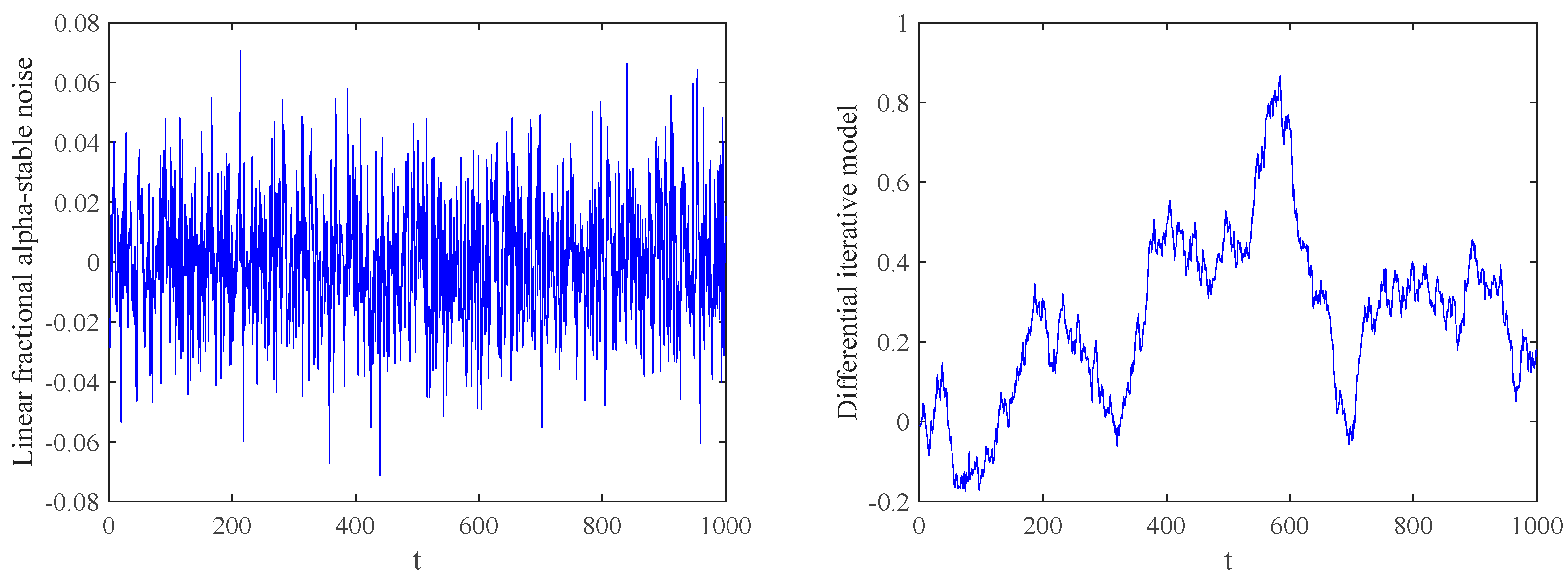
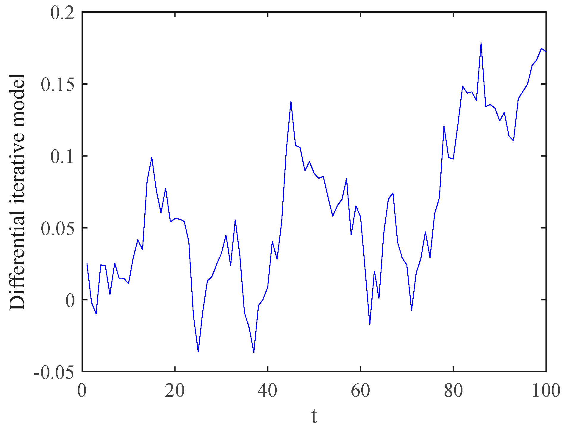
Finally, the iterative difference prediction model based on the LFSM model is obtained in Equation (25). Figure 5 shows the numerical simulation of the model.
L α , H t + 1 = L α , H t + μ L α , H t t + δ L α , H t w a ( t ) ( t ) H

4.2. Existence and Uniqueness for the Solution of the Model

Since the accuracy of the actual measured initial data cannot be guaranteed and it is not certain that the tested initial data can be used as the true solution, this subsection discusses the Cauchy problem of Equation (25) or Equation (18), by proving the existence and uniqueness of its solution to the initial value problem. Furthermore, if the initial value creates a negligible small change or its solution similarly produces a negligible small change, the solution’s consistent convergence must be considered.
To ensure that Equation (18) can describe the uncertain variation of a random sequence, the process should be guaranteed to have a unique solution. We abbreviate Equation (18) as follows:
d S t = S t ( μ d t + δ d L t ) S t = 0 = S 0
where L t = 0 t ( t s ) a d W s follows the definition in Section 3 and a semimartingale L t ε = 0 t ( t s + ε ) a d W s that consistently converges to L t has been obtained. Substituting the semimartingale L t ε into Equation (26) provides:
d S t ε = S t ε ( μ d t + δ d L t ε ) S t = 0 ε = S 0 ε > 0
We have obtained the following two Corollaries.
Since Equation (27) is a semimartingale process, its solution may be obtained using the Ito formula.
Corollary 3.
The solution of Equation (27) is
S t ε = S 0 e x p δ ε a + 1 2 δ 2 ε 2 a t + 0 t h s ε d s
where  a = H 1 α h s ε = μ + a δ 0 t ( t s + ε ) a 1 d W s , assuming that the initial value  S t = 0 ε  is a bounded random variable.
Corollary 4.
When the stochastic process is in  L 2 ( Ω ) , and  ε 0 ,
S t * = S 0 e x p ( μ t + δ L t )
This is the solution of Equation (26).
Proof. 
According to Equation (27), we can get
d L t ε = d a 0 t Φ t ε d s + ε a W t = 0 t a ( t s + ε ) a 1 d W s d t + ε a d W t
Substitute Equation (30) into Equation (28)
d S t ε = S t ε μ + a δ 0 t a ( t s + ε ) a 1 d W s d t + ε a δ S t ε d W t = S t ε h t ε d t + ε a δ S t ε d W t
Obviously, here is
h t ε = μ + a δ 0 t t s + ε a 1 d W s
Equation (20) can be written as
d S t ε S t ε = h t ε d t + ε a δ d W t
Using Ito formula for the above equation
log S t ε = log S 0 ε + 0 t d S t ε S t ε + 1 2 0 t 1 S s ε 2 ε a δ S s ε 2 d s
From the above equation, we get
S t ε = S 0 e x p δ ε a + 1 2 δ 2 ε 2 a t + 0 t h s ε d s
Therefore, Corollary 3 is proved. □
Proof. 
According to Equation (35), in order to further simplify, it takes
0 t h s ε d s = μ t + δ a 0 t 0 s s u + ε a 1 d W u d s
0 t 0 s s u + ε a 1 d W u d s = 0 t u s s u + ε a 1 d s d W u = 1 a 0 t s u + ε a d W u ε a W t = 1 a L t ε ε a
Gathering Equations (36) and (37), we obtain
0 t h s ε d s = μ t δ ε a + δ L t ε
So that
S t ε = S 0 e x p ( 1 2 δ 2 ε 2 a t + μ t + δ L t ε )
By putting ε 0 in the above equation, we can get:
S t * = S 0 e x p ( μ t + δ L t )
According to Equation (40), after obtaining the approximation solution, it is necessary to verify that the solution consistently converges to Equation (39) to ensure that when a small change in S t * occurs in the L 2 ( Ω ) region, a small change in S t ε can follow accordingly.
In the following, we will prove that S t ε converges uniformly to S t * .
S t ε S t * = S 0 exp 1 2 δ 2 ε 2 a t + μ t + δ L t ε S 0 e x p ( μ d t + δ L t ) = S 0 e x p ( μ d t + δ L t ) exp 1 2 δ 2 ε 2 a t + δ L t ε L t 1
According to L t = 0 t ( t s ) a d W s , we can get
L t 2 = E ( 0 t ( t s ) a d W s ) 2 = t 1 + 2 a 1 + 2 a
From the above equation, in t [ 0 , T ] , we can see that
e x p ( μ d t + δ L t ) e μ t exp δ L t e μ T exp δ T 1 2 + a 1 + 2 a
According to the equation e A 1 = A + o ( A ) , the other half of Equation (41) has the following relationship
exp 1 2 δ 2 ε 2 a t + μ L t ε L t 1 1 2 δ 2 ε 2 a t + δ L t ε L t + o L t ε L t
Combining Equation (15)
exp 1 2 δ 2 ε 2 a t + μ L t ε L t 1 δ 2 ε 2 a T + C ( a ) ε 1 + 2 a
Considering Equations (41), (43), and (45) together, the following results can be obtained
S t ε S t * e μ T e x p δ T 1 2 + a 1 + 2 a δ 2 ε 2 a T + C ( a ) ε 1 + 2 a 0 sup 0 t T
So, Corollary 4 is proved. □
It is also important to demonstrate the uniqueness of Equation (18)’s solution in order to verify that it can be merged with a random sequence of fractional-order stable Lévy white noise.
S t * ( 1 ) S t * ( 2 ) S t * 1 S t ε + S t * 2 S t ε 0   a . s . ε 0
If S t * 1 and S t * ( 2 ) are limits of S t ε in L 2 ( Ω ) , then this solution is unique.
In summary, Equation (25), the solution of the LFSM differential iterative model proposed in this paper, is demonstrated in this section using a semimartingale approximation, proving that the model is reasonable at the theoretical level and can describe the uncertain variation of stochastic sequences.

4.3. Parameter Estimation of LFSM Degradation Model

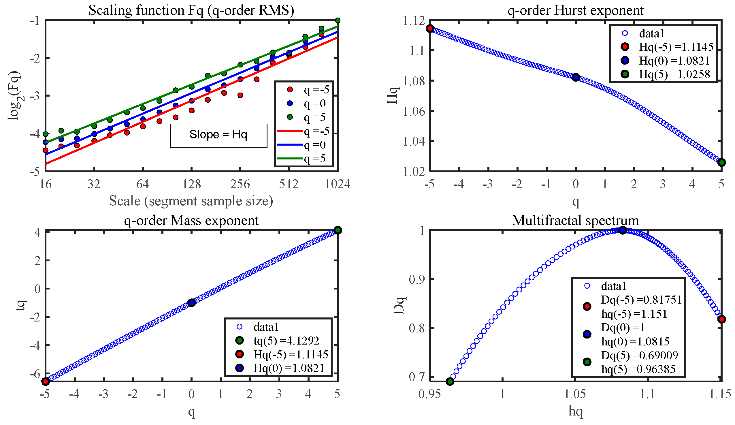
The algorithms for estimating the values of H are primarily divided into two categories: time domain analysis methods, which generally calculate the sample series directly and then obtain the estimated values of Hurst parameters by curve fitting, primarily the variance method, rescaled polar difference method, and absolute value method, etc.; and frequency domain analysis methods, which primarily use Fourier changes to transform the sample data into the frequency domain. The rescaled polar difference method is used in this paper to estimate H, because the implementation process is very simple, and the calculation is simple and easy to understand; the specific process is as follows:
Step 1: The sample input data X t , t = 1,2 , of length n is divided into h submodules of equal length (all of which are a), and the mean value of each submodule is determined;
X a = 1 a i = 1 d X i
Step 2: Calculate the cumulative deviation for each submodule;
X i , a = p = 1 d X p X a
Step 3: Calculate the extreme differences for each submodule;
R a = X i , a   max 1 i a X i , a   min 1 i a
Step 4: Calculate the standard deviation of each submodule;
S a = 1 a p = 1 d X p X a 2
Step 5: Divide the polar deviation of each submodule by the standard deviation and average it to get the rescaled polar deviation of each submodule;
R S a = 1 h × R ( a ) S ( a )
Step 6: The supplied sample data is rescaled into submodules. As long as h × a = n is met, a can take different values, and then Steps 1–5 can be repeated to achieve different rescaled polar deviations;
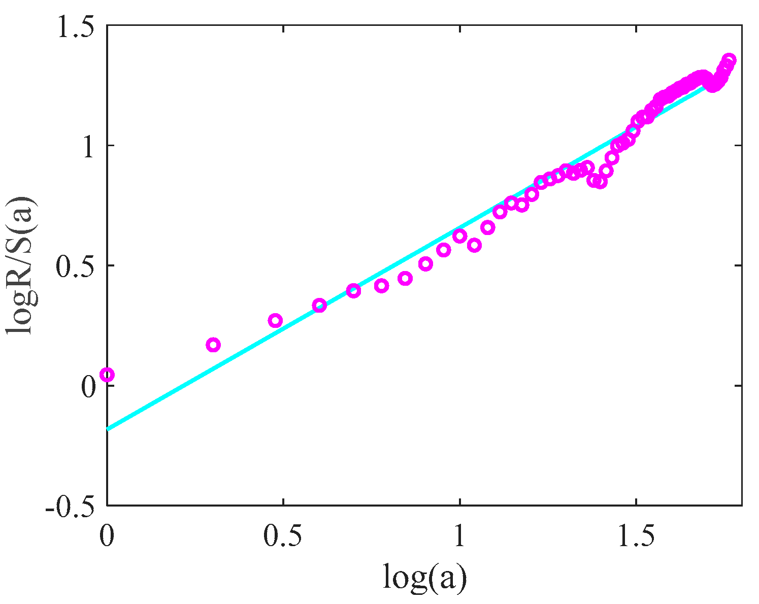
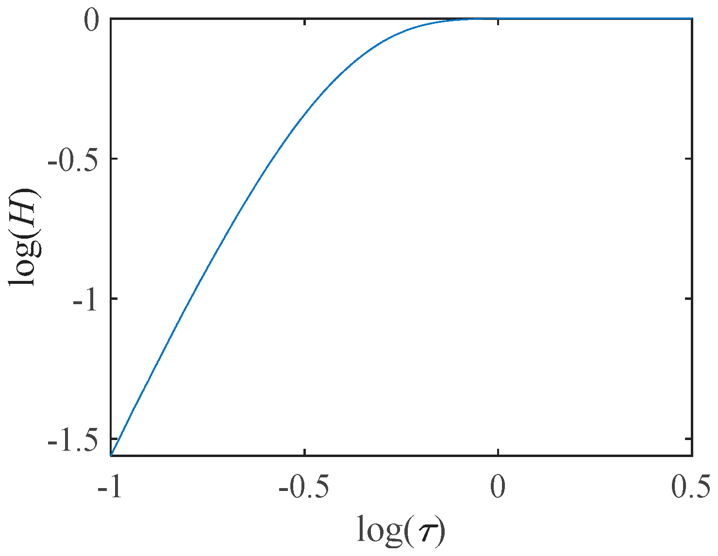
Step 7: Logarithmize each submodules’ length a and the accompanying R S ( a ) to produce log R S ( a ) and log a, and then fit them using least squares, as shown in Figure 6.
log R S ( a ) = log c + H × log a + ω
Figure 6 shows the slope’s H, which is the projected value required in this paragraph.
There are still four parameters with values to be estimated, which are diffusion parameter δ, stability index α, skewness index β, and drift coefficient μ. In this paper, we use the new eigenfunction estimation method. The specific steps are shown in [39,40].
The LFSM model, in contrast with the standard Gaussian process that obeys the central limit theorem, is a non-Gaussian process that obeys the modified central limit theorem and lacks a PDF expression in the usual sense of a restricted form. The LFSM model includes an explicit eigenfunction to address the issue of difficult parameter solutions caused by the PDF’s lack of a restricted form. The PDF of the LFSM model may be produced by applying Fourier transforms on the eigenfunctions. As a result, the parameter estimate may be increased using the eigenfunctions. There is one point you should keep in mind, θ 1 = 1 . This is because the absolute values of the eigenfunctions are equivalent at location θ 1 = 1 , regardless of the eigenfunction parameters’ values.
φ 1 ; α , β , δ , μ = e δ
Additionally, there is a crucial point θ 2 that calculates using α = 1 and α = 2 , which stands for the Cauchy and Gaussian eigenfunctions.
d d θ e δ θ 2 e δ θ = 0
2 θ e δ θ 2 = e δ θ
Assuming that the input sequence is X = x 1 , x 2 , , x n :
Step 1: Estimate the value of δ , Equation (54)’s logarithmic likelihood estimate;
δ ^ = ln φ ^ 1 ; α , β , δ , μ = ln 1 N i = 1 N e j x i
Step 2: Estimate the value of α, combining Equation (56) and Equation (55);
α ^ = log θ 2 ( ln φ ^ ( θ 2 ; α , β , δ , μ ) ln φ ^ ( 1 ; α , β , δ , μ ) ) ln φ ^ ( θ 2 ; α , β , δ , μ ) ln φ ^ ( 1 ; α , β , δ , μ ) ln θ 2 φ ^ θ 2 ; α , β , δ , μ = 1 N i = 1 N e j x i
Step 3: Estimate the value of μ, the logarithmic version of the characteristic function which is used to obtain the estimate of the drift coefficient.
ln φ θ ; α , β , δ , μ = j μ θ + θ α δ β θ θ tan π α 2 δ θ α
With the help of the two points θ 1 and θ 2 , the estimated value can be obtained
μ ^ = Im { θ 2 α ^ ln φ ^ ( 1 ; α , β , δ , μ ) ln φ ^ ( θ 2 ; α , β , δ , μ ) } θ 2 α θ 2
Since the LFSM model used in this work has a symmetric driving function, β ^ = 0 in this model.

5. Feature Extraction Using PCA and MLE

PCA is a multivariate statistics-based analytic approach whose basic principle is to orthogonally convert information from high-dimensional to low-dimensional subspaces and reorganize the original indicators into a new set of uncorrelated composite indicators.
The steps of the method are as follows:
Step 1: Use the z-score to standardize the original data;
Step 2: Calculate the sample matrix’s covariance matrix;
Step 3: Solve the covariance matrix’s eigenroots and eigenvectors;
Step 4: Determine the primary element matrix.
In brief, the determination of principal components is divided into the following processes, as seen in Figure 7.
Following PCA data fusion, a typical feature degradation sequence is created, and the MLE is used to determine the maximum prediction length appropriate for that curve.
The principle of modelling the Lyapunov Exponent using the small data size method is as follows:
For a time series y i , i = 1,2 , , n with embedding dimension m y , time delay τ y , and average period P y , the reconstructed phase space is
Y i = y i , y i + τ y , , y ( i + ( m y 1 ) τ y ) , i = 1,2 , , M y
For each reference point Y ( j ) , the distance to its nearest neighbor Y ( j ) after the n i ( n = 1,2 , 3 , ) discrete time step is calculated as
d j j n i = Y j Y ( j )
where i = 1,2 , , m i n M y j n , M y j n , j j > P y , P y is the average period of the time series.
Assume that the reference point Y j ’s exponential divergence from its nearest neighbor Y ( j ) is 1 , then
ln d j j n i = ln d j j 0 + 1 ( i t )
Fixing i for every ln d j j n i is averaged and divided by t to produce the average divergence index
s i = 1 q t k = 1 q ln d j k j k n i
where q is non-zero d j k j k ( k = 1 , 2 , . . . , q ) in number. Using the least squares method to make the regression straight, the LLE can be found by calculating the slope of the line as 1 . Figure 8 shows the upper part with s i and the lower part with the slope.
Calculation of maximum Lyapunov coefficient by small data method ϑ :
ϑ = ln d j j n i ln d j j 0 i t
The maximum prediction range of the degenerate feature sequence can be obtained by the inverse of the maximum Lyapunov coefficient ϑ
= 1 ϑ
The calculation steps are shown in Figure 9:
After determining the degradation sequence and maximum prediction length, the degradation trend may be forecasted using the LFSM model, which is explained in the following section.

6. Fractal Dimension and MDFA

Grassberger and Procaccia proposed a calculation method in 1983 based on the idea of phase space reconstruction [41]. The method is based on the idea of using distances to characterize the degree of points correlation in a set. For set X x 1 , x 2 , , x n , the steps of the method are as follows:
Step 1: Calculation of correlation function
S τ = 1 n 2 i j n s ( τ x i x j )
where x i x j is Euclidean parametrization, τ is constant, and;
h τ x i x j = 1 , τ x i x j 0 , τ < x i x j
Step 2: Fractal dimension D is
D = lim τ 0 log H τ log τ
The MDFA is as follows:
Step 1: Calculate the sum of x i and the mean value;
y i = i = 1 n ( x i x ) , n = 1,2 , , N
Step 2: Divide y into independent subsequences of length s, with a total of m,  m = i n t ( N / s ) . Use least squares to fit the local trend of the subsequences;
y v i = a 0 + a 1 i + a 2 i 2 + + a k i k , i = 1,2 , ; k = 1,2 ,
Step 3: To eliminate local trends, calculate the mean square error function;
F 2 u , s = 1 s i = 1 s ( y v 1 s + i y v i ) 2 , u = 1,2 , , m
F 2 u , s = 1 s i = 1 s y N v 1 s + i y v i 2 , u = m + 1 , m + 2 , , 2 m
Step 4: Calculating the q-order fluctuation function. It has a power-law relationship with the generalized hurst exponent, F q ( s ) ~ s h ( q ) .
F q s = 1 2 m u = 1 2 m F 2 u , s q / 2 1 / q

7. Case Study

The LFSM differential iterative model is verified with multi-sensor end mill monitoring data (Cut 6) from the Roders Tech RFM760 high-speed CNC milling machine during the PHM 2010 Challenge [35]. The experimental platform is shown in Figure 10, with 315 tool walks and 69,139,039 data points. Table 1 provides the essential instrument specifications. Figure 11 is the initial vibration signal.
The wear of end mills can be distinguished into three different stages depending on the rapid change in wear rate: initial stage, steady stage, and sharp stage. The offline measurement of the tool wear value VB on the cutting edge during the process from cutting into the workpiece to full cutting out is shown in Figure 12 using a LEICA MZ12 HD microscope.
When it is in the initial stage, the cutting edge is sharp, and the tool often vibrates violently. Figure 12 shows that the slope of the curve at this stage is greater, indicating a faster rate of wear. This is mainly caused by the insufficiently steady contact between the tool and the workpiece during this time, which indirectly contributes to the instability of the cutting process and causes the tool to wear out more quickly during this time. The wear during this period is minimal, averaging between 0.05 and 0.1 mm.
When the tool is in the steady stage, the contact area between the workpiece and the tool surface increases and the tool gradually hardens. The compressive stress is also reduced. The cutting process is more stable, the surface of the workpiece is smoother, and the amount of vibration generated is less. Figure 12 depicts those conclusions under the steady stage, as the tool wear curve has a modest slope, a steady wear rate, and a long usage time.
Figure 12 shows that as the machining time is increased, the tool wears more quickly, the slope of the rapid wear period curve increases, and the tool eventually reaches the failure state.
In order to ensure correct machining and increase efficiency, the vibration signal is used to monitor the state of wear in order to detect and replace new tools in a timely manner before the sharp stage arrives.
Therefore, in Figure 12, the maximum average wear VB value of 0.15 mm is set as the failure threshold, and the number of tool walks to 70 to enter the steady stage and 200 to enter the sharp stage. The condition of the tool is determined by the amount of wear described in ISO 3685, ISO 8688, and ANSI/ASME B94.55M [42]. In [42], the VB value reaches half of the tool’s radius when it is worn blunt. Figure 13 depicts the prediction process utilized in this paper.

7.1. Extracting Feature Parameters

In Figure 14, 10 time-frequency domain parameters are chosen and calculated: mean of absolute values, variance, kurtosis, margin factor, crest factor, impulse factor, waveform factor, vibration velocity energy, vibration intensity, and mean of power spectrum. Figure 11 has undergone a total of 315 walks. In order to quickly predict the wear of the tool, this paper calculates the above ten characteristics’ quantities from the vibration data for each tool walk. At this point, the tool wear degradation is analyzed by using the 315 data trends for each of the ten characteristics’ quantities.
In this study, the above time-domain features were characteristically fused using PCA, and the analysis results are shown in Figure 15. According to Figure 15, the first five main components account for 95% of the entire contribution, indicating that the deterioration trend can be described by the feature information of the first five principal components.
Table 2 displays the dimensionality reduction findings for each primary component, and Figure 15 displays the histogram. The degraded feature sequence for feature fusion is shown in Figure 16.
Smoothing the degradation sequence shown in Figure 16 into Figure 17, it can be seen from Figure 12 that we will predict the degradation trend from initial wear to normal wear (starting at a tool walk count of 70) and from normal wear to sharp wear (starting at a tool walk count of 200).

7.2. Fractal Dimension Calculation

According to Section 6, the fractal dimension of the vibration signal can be obtained by using Equations (67)–(69). The relationship between log H ( τ ) and log τ is shown in Figure 18.
As in Figure 18, the fractal dimension can be obtained as 1.3984, and the results show that the evolution of the tool wear condition shows self-similarity. In Section 2.2, the LFSM has the same characteristic. Additionally, the LFSM has LRD, which takes full account of historical data to allow for tmore accurate predictions of vibration signals.

7.3. Degradation Process Prediction

Firstly, the vibration signal from the initial stage to the steady stage is predicted, and it is known that the tool starts to enter the steady stage when the number of tool walks reaches 70, at which point the MLE is shown in Table 3, giving a maximum prediction step size of 97. The prediction is fully achievable. Figure 19 shows a comparison with the fuzzy neural network (FNN) method from the literature [35], the LSTM method traditionally used for predicting time series, and the fBm method, which is most commonly used in the field of LRD. In order to show the results more visually, this paper only shows the predicted part. The parameters of the LFSM differential iterative model and the fBm model are shown in Table 4, and Table 5 shows the analysis of the performance. Five evaluation criteria were used to compare the results: maximum error (MAX), mean error (MEAN), standard error (STD), Score of Accuracy (SOA), and Health Degree (HD).
Let x i refers to real data, x I ^ refers to predicted data, and x I refers to the real data’s mean. The total number is n, and i = 1,2 , , n .
(1) maximum error (MAX), indicates the maximum value of the relative error:
M a x = m a x x i x I ^
(2) mean error (MEAN), indicates the mean of relative error:
M e a n = 1 n i = 1 n x i x I ^
(3) standard error (STD)
S t d = 1 n 1 i = 1 n x i x I 2 1 / 2
(4) Score of Accuracy (SOA), indicates the fit ratio of model, S O A is the mean of all of S O A i :
S O A i = exp ln 0.5 E r i / 20 , E r i > 0 exp ln 0.5 E r i / 5 , E r i < 0
E r i = 100 × x i x I ^ x i
(5) Health Degree (HD), a health index closer to 1 indicates better performance of the prediction model:
H D = 1 i = 1 n ( x i x I ^ ) i = 1 n ( x i x I )
From Figure 19 and Table 5, it can be seen that the LFSM prediction model is better than fBm and other methods in predicting from the initial stage to the steady stage.
Next, predicting the pattern from the steady stage to the sharp stage. When the number of tool steps reaches 200, the tool enters the condition of sharp stage, and the maximum Lyapunov index at this time is indicated in Table 6, which obtained the highest prediction step of 90. Table 7 shows the parameters of the two prediction models, LFSM and fBm, and Table 8 evaluates the prediction models’ qualities. Figure 20 depicts the results; again, only the predicted part is shown.
Similarly, using Figure 20 and Table 8, it is possible to conclude that the LFSM prediction model is more accurate than the fBm prediction model and other models in the transition from the steady stage to the sharp stage.
From Table 4 and Table 7, it can be seen that the Hurst index of the vibration signal is different at various wear stages, and it is calculated that at the initial stage, its Hurst index is 0.7873, therefore, the Hurst index can reflect the failure state of the tool. In a one-dimensional space, the relationship between the Hurst index and fractal dimension D is H + D = 2 .

7.4. Monitoring the Value of VB

According to Section 7.3, the Hurst index can reflect the wear state. In this section, Multiple Fractal Detrended Fluctuation Analysis (MDFA) [43] is used to analyze the vibration signals obtained from previous predictions, obtain the eigenvectors reflecting changes in VB values, i.e., the generalized Hurst index, and train the ECoS neural network with the health factor from Section 7.1 for wear detection. The data from PHM 2010 is still used in this case to monitor the VB value of cut 1 with cut 6. Figure 21 shows the flow of MDFA. The results of cut 6 are shown in Figure 22. According to the MDFA algorithm, the parameters of the initial stage, steady stage, and sharp stage are found out, respectively, and Figure 22 shows the parameters of the sharp stage.
The data obtained from cut 6 was substituted into the ECoS model that was trained to monitor the wear of cut 1, and the results in Figure 23 were obtained. It was verified that the correct rate reached 98.7%, which is much higher than the accuracy of the traditional neural network.

8. Conclusions

The prediction of tool wear can increase efficiency and save costs. This paper uses PCA and MLE to analyze the data, constructing LFSM differential iterative models to implement predicted vibration signals. Firstly, the general solution of the stochastic integral is obtained by constructing a semimartingale, and the model has theoretically proved to integer order the Ito stochastic integral. Then, the maximum prediction step derived by MLE, estimated model parameters, and the LFSM differential iterative model were constructed using historical end mill tool vibration data. Using PCA signal fusion, the key component signals influencing tool vibration were identified, and the prediction results were compared with the fBm approach, FNN method, and LSTM method. The LFSM-based prediction model was proven to be useful and effective. From the experimental results, it can be seen that the LFSM prediction method studied in this paper not only has better accuracy than the FNN method in [26], or the traditional time series prediction method LSTM, or the fBm method, which is widely used in long related fields nowadays, but the LFSM iterative prediction model can better accomplish the prediction. Moreover, the α parameter was added to be compared with the fBm method, which makes the model more flexible. Finally, this paper uses MDFA on the vibration signals predicted in the previous paper to obtain the association between the generalized Hurst index and the wear state, and utilizes the ECoS model for VB value prediction.
The suggested model improves upon the degradation trend prediction approach, although it still has limitations, and the prediction experiments were acquired through degradation testing on an experimental rig in a simulated real-world operating environment. The actual plant equipment functions in a more complicated environment, despite the setting of various operational parameters. In a multi-state situation, the data preprocessing approach suggested in this paper cannot achieve optimal feature extraction, and further analysis of the raw data is necessary. Furthermore, this study only uses one set of degraded data to evaluate the suggested prediction model, although it may be helpful to incorporate many various types of degraded data to test the model’s prediction performance.

Author Contributions

All authors equally contributed to carrying out the research, whose results are reported in this work. All authors have read and agreed to the published version of the manuscript.

Funding

The contribution of A. Kudreyko was supported by PRIORITY-2030 (Bashkir State Medical University).

Data Availability Statement

Not applicable.

Conflicts of Interest

The authors declare no conflict of interest.

Acronyms and Abbreviations

LFSMLinear fractional alpha-stable motion
PCAPrincipal component analysis
MLEMaximum Lyapunov exponent
MDFAMultifractal detrended fluctuation analysis
ECoSEvolving connectionist system
LRDLong-range dependence
FNNFuzzy neural network
LSTMLong-short term memory
fBmFractional Brownian motion
VBValue of bandwidth
HHurst index

References

  1. Javed, K.; Gouriveau, R.; Li, X.; Zerhouni, N. Tool wear monitoring and prognostics challenges: A comparison of connectionist methods toward an adaptive ensemble model. J. Intell. Manuf. 2018, 29, 1873–1890. [Google Scholar] [CrossRef]
  2. Vetrichelvan, G.; Sundaram, S.; Kumaran, S.S.; Velmurugan, P. An investigation of tool wear using acoustic emission and genetic algorithm. J. Vib. Control. 2015, 21, 3061–3066. [Google Scholar] [CrossRef]
  3. Zhu, K.; Yu, X. The monitoring of micro milling tool wear conditions by wear area estimation. Mech. Syst. Signal Process. 2017, 93, 80–91. [Google Scholar] [CrossRef]
  4. Szydłowski, M.; Powałka, B.; Matuszak, M.; Kochmański, P. Machine vision micro-milling tool wear inspection by image reconstruction and light reflectance. Precis. Eng. 2016, 44, 236–244. [Google Scholar] [CrossRef]
  5. Choudhury, S.K.; Srinivas, P. Tool wear prediction in turning. J. Mater. Process. Technol. 2004, 153, 276–280. [Google Scholar] [CrossRef]
  6. Salgado, D.; Alonso, F. Tool wear detection in turning operations using singular spectrum analysis. J. Mater. Process. Technol. 2006, 171, 451–458. [Google Scholar] [CrossRef]
  7. Elangovan, M.; Devasenapati, S.B.; Sakthivel, N.; Ramachandran, K. Evaluation of expert system for condition monitoring of a single point cutting tool using principle component analysis and decision tree algorithm. Expert Syst. Appl. 2011, 38, 4450–4459. [Google Scholar] [CrossRef]
  8. Gong, W.; Li, W.; Shirakashi, T.; Obikawa, T. An active method of monitoring tool wear states by impact diagnostic excitation. Int. J. Mach. Tools Manuf. 2004, 44, 847–854. [Google Scholar] [CrossRef]
  9. Hanachi, H.; Yu, W.; Kim, I.Y.; Liu, J.; Mechefske, C.K. Hybrid data-driven physics-based model fusion framework for tool wear prediction. Int. J. Adv. Manuf. Technol. 2019, 101, 2861–2872. [Google Scholar] [CrossRef]
  10. Palanikumar, K.; Davim, J.P. Mathematical model to predict tool wear on the machining of glass fibre reinforced plastic composites. Mater. Des. 2007, 28, 2008–2014. [Google Scholar] [CrossRef]
  11. Yang, S.; Zhu, G.; Xu, J.; Fu, Y. Tool wear prediction of machining hydrogenated titanium alloy Ti6Al4V with uncoated carbide tools. Int. J. Adv. Manuf. Technol. 2013, 68, 673–682. [Google Scholar] [CrossRef]
  12. Zhang, C.; Zhang, H. Modelling and prediction of tool wear using LS-SVM in milling operation. Int. J. Comput. Integr. Manuf. 2016, 29, 76–91. [Google Scholar] [CrossRef]
  13. Song, X.; Shuai, S.; Bo, L. Adaptive synchronization of two time-delayed fractional-order chaotic systems with different structure and different order. Opt.-Int. J. Light Electron Opt. 2016, 127, 11860–11870. [Google Scholar] [CrossRef]
  14. Mandelbrot, B.B.; Aizenman, M. Fractals: Form, Chance, and Dimension. Phys. Today 1979, 32, 65–66. [Google Scholar] [CrossRef]
  15. Sayles, R.S.; Thomas, T.R. Surface topography as a nonstationary random process. Nature 1978, 271, 431–434. [Google Scholar] [CrossRef]
  16. Majumdar, A.; Bhushan, B. Role of Fractal Geometry in Roughness Characterization and Contact Mechanics of Surfaces. J. Tribol. 1990, 112, 205–216. [Google Scholar] [CrossRef]
  17. Oldham, K.B.; Spanier, J. The fractional calculus. In Theory and Applications of Differentiation and Integration to Arbitrary Order; Academic Press: New York, NY, USA, 2006. [Google Scholar]
  18. Ma, C.; Hori, Y. Fractional Order Control and Its Application of PI~αD Controller for Robust Two-inertia Speed Control. In Proceedings of the 4th International Power Electronics and Motion Control Conference (IPEMC 2004), Xi’an, China, 14–16 August 2004; Volume 3. [Google Scholar]
  19. Júnior, A.A. Backward inducing and exponential decay of correlations for partially hyperbolic attractors. Isr. J. Math. 2002, 130, 29–75. [Google Scholar]
  20. Ehleringer, J.R.; Field, C.B. Scaling Physiological Processes: Leaf to Globe. J. Ecol. 1993, 44, 388. [Google Scholar]
  21. Liu, H.; Song, W.; Zio, E. Generalized Cauchy difference iterative forecasting model for wind speed based on fractal time series. Nonlinear Dyn. 2021, 103, 759–773. [Google Scholar] [CrossRef]
  22. Liu, H.; Song, W.; Zhang, Y.; Kudreyko, A. Generalized Cauchy Degradation Model with Long-Range Dependence and Maximum Lyapunov Exponent for Remaining Useful Life. IEEE Trans. Instrum. Meas. 2021, 70, 3512812. [Google Scholar] [CrossRef]
  23. Bayraktar, E.; Poor, H.V.; Rao, R. Prediction and tracking of long-range-dependent sequences. Syst. Control. Lett. 2005, 54, 1083–1090. [Google Scholar] [CrossRef]
  24. Duan, S.; Song, W.; Zio, E.; Cattani, C.; Li, M. Product technical life prediction based on multi-modes and fractional Lévy stable motion. Mech. Syst. Signal Process. 2021, 161, 107974. [Google Scholar] [CrossRef]
  25. Song, W.; Liu, H.; Zio, E. Long-range dependence and heavy tail characteristics for remaining useful life prediction in rolling bearing degradation. Appl. Math. Model. 2022, 102, 268–284. [Google Scholar] [CrossRef]
  26. Li, Y.; Song, W.; Wu, F.; Zio, E.; Zhang, Y. Spectral Kurtosis of Choi–Williams Distribution and Hidden Markov Model for Gearbox Fault Diagnosis. Symmetry 2020, 12, 285. [Google Scholar] [CrossRef] [Green Version]
  27. Li, M. Fractal time series—A tutorial review. Math. Probl. Eng. 2010, 2010, 157264. [Google Scholar] [CrossRef] [Green Version]
  28. Laskin, N.; Lambadaris, I.; Harmantzis, F.; Devetsikiotis, M. Fractional Lévy motion and its application to network traffic modeling. Comput. Netw. 2002, 40, 363–375. [Google Scholar] [CrossRef] [Green Version]
  29. Weron, A.; Burnecki, K.; Mercik, S.; Weron, K. Complete description of all self-similar models driven by Lévy stable noise. Phys. Rev. E 2005, 71, 016113. [Google Scholar] [CrossRef] [Green Version]
  30. Black, F.; Scholes, M. The Pricing of Options and Corporate Liabilities. J. Politi-Econ. 1973, 81, 637–654. [Google Scholar] [CrossRef] [Green Version]
  31. Jumarie, G. On the representation of fractional Brownian motion as an integral with respect to (dt) a. Appl. Math. Lett. 2005, 18, 739–748. [Google Scholar] [CrossRef] [Green Version]
  32. Rosenstein, M.T.; Collins, J.J.; De Luca, C.J. A practical method for calculating largest Lyapunov exponents from small data sets. Phys. D Nonlinear Phenom. 1993, 65, 117–134. [Google Scholar] [CrossRef]
  33. Adeyemo, O.D.; Khalique, C.M.; Gasimov, Y.S.; Villecco, F. Variational and non-variational approaches with Lie algebra of a generalized (3 + 1)-dimensional nonlinear potential Yu-Toda-Sasa-Fukuyama equation in Engineering and Physics. Alex. Eng. J. 2023, 63, 17–43. [Google Scholar] [CrossRef]
  34. Li, X.; Er, M.J.; Lim, B.S.; Zhou, J.H.; Gan, O.P.; Rutkowski, L. Fuzzy regression modeling for tool performance prediction and degradation detection. Int. J. Neural Syst. 2010, 20, 405–419. [Google Scholar] [CrossRef] [PubMed]
  35. Li, X.; Lim, B.S.; Zhou, J.H.; Huang, S.; Phua, S.J.; Shaw, K.C.; Er, M.J. Fuzzy neural network modelling for tool wear estimation in dry milling operation. In Proceedings of the Annual Conference of the PHM Society, San Diego, CA, USA, 27 September–1 October 2009. [Google Scholar]
  36. Zou, H.-L.; Yu, Z.-G.; Anh, V.; Ma, Y.-L. From standard alpha-stable Lévy motions to horizontal visibility networks: Dependence of multifractal and Laplacian spectrum. J. Stat. Mech. Theory Exp. 2018, 2018, 053403. [Google Scholar] [CrossRef]
  37. Samorodnitsky, G.; Taqqu, M.S. Stable Non-Gaussian Random Processes: Stochastic Models with Infinite Variance: Stochastic Modeling; Routledge: London, UK, 2017. [Google Scholar]
  38. Gallardo, J.R.; Makrakis, D.; Orozco-Barbosa, L. Use of α-stable self-similar stochastic processes for modeling traffic in broadband networks. Perform. Eval. 2000, 40, 71–98. [Google Scholar] [CrossRef]
  39. Xing, J.; Song, W.; Villecco, F. Generalized Cauchy Process: Difference Iterative Forecasting Model. Fractal Fract. 2021, 5, 38. [Google Scholar] [CrossRef]
  40. Bibalan, M.H.; Amindavar, H.; Amirmazlaghani, M. Characteristic function based parameter estimation of skewed alpha-stable distribution: An analytical approach. Signal Process. 2017, 130, 323–336. [Google Scholar] [CrossRef]
  41. Xu, C.; Hualing, C. Fractal analysis of vibration signals for monitoring the condition of milling tool wear. Proc. Inst. Mech. Eng. Part J-J. Eng. Tribol. 2009, 223, 909–918. [Google Scholar]
  42. Sick, B. On-line and indirect tool wear monitoring in turning with artificial neural networks: A review of more than a decade of research. Mech. Syst. Signal Process. 2002, 16, 487–546. [Google Scholar] [CrossRef]
  43. Ihlen, E.A.F. Introduction to Multifractal Detrended Fluctuation Analysis in Matlab. Front. Physiol. 2012, 3, 141. [Google Scholar] [CrossRef] [Green Version]
Figure 1. (a) Effects of different α. (b) Effects of different β.
Fractalfract 07 00325 g001
Figure 2. (a) Effects of different μ. (b) Effects of different δ.
Fractalfract 07 00325 g002
Figure 3. Simulation sequence of LFSM numerical series.
Fractalfract 07 00325 g003
Figure 4. The series of LFSM noise and LFSM.
Fractalfract 07 00325 g004
Figure 5. Simulation of differential iterative model.
Fractalfract 07 00325 g005
Figure 6. Least squares fitting.
Fractalfract 07 00325 g006
Figure 7. The PCA processes.
Fractalfract 07 00325 g007
Figure 8. The least-squares regression and slope of s(i).
Fractalfract 07 00325 g008
Figure 9. MLE Calculations.
Fractalfract 07 00325 g009
Figure 10. Schematic diagram of the PHM experimental platform.
Fractalfract 07 00325 g010
Figure 11. The original vibration signals.
Fractalfract 07 00325 g011
Figure 12. The value of bandwidth at different stages.
Fractalfract 07 00325 g012
Figure 13. The prediction technique.
Fractalfract 07 00325 g013
Figure 14. Time and frequency domain characteristics.
Fractalfract 07 00325 g014
Figure 15. The outcomes of each primary component.
Fractalfract 07 00325 g015
Figure 16. Feature sequences.
Fractalfract 07 00325 g016
Figure 17. The smoothing feature sequences.
Fractalfract 07 00325 g017
Figure 18. The relationship between log H(τ) and log τ.
Fractalfract 07 00325 g018
Figure 19. Predicted results from the initial stage to the steady stage.
Fractalfract 07 00325 g019
Figure 20. Predicted results from the steady stage to the sharp stage.
Fractalfract 07 00325 g020
Figure 21. MDFA algorithm.
Fractalfract 07 00325 g021
Figure 22. The parameter of sharp stage by MDFA.
Fractalfract 07 00325 g022
Figure 23. Cut 1’s VB value monitoring results.
Fractalfract 07 00325 g023
Table 1. Basic parameters of the tools.
Basic ParameterParameter ValueBasic ParameterParameter Value
PlatformRoders Tech RFM 760Total cuts315
Depth of cut0.125 mmSpindle speed10,400 rpm/min
Types of sensorsVibrationMaterialStainless steel
Sampling frequency50 kHzType of toolCarbid ball Φ 6 mm
Table 2. The outcomes of each primary component’s dimensionality reduction.
PortionsF1F2F3F4F5F6F7F8F9F10
Eigenvalues5.58961.33701.20060.88160.49280.36490.12580.007800
Contribution 0.55900.13370.12010.08820.04930.03650.0126000
Table 3. Maximum Lyapunov exponent parameters from the initial stage to the steady stage.
myτy Maximum Prediction Step
860.010397
Table 4. Parameters of the LFSM and the fBm model from the initial stage to the steady stage.
ModelsHαβμδ
LFSM0.83391.312102.69110.0405
fBm0.8339\\2.49670.0241
Table 5. Performance analysis from the initial stage to the steady stage.
ModelsMAXMEANSTDSOAHD
LFSM0.58910.04040.01720.91540.9862
fBm0.57050.11220.14390.85730.9431
FNN0.49560.01990.18870.49220.8940
LSTM3.10500.20790.65760.2658−2.4910
Table 6. Maximum Lyapunov exponent parameters from the steady stage to the sharp stage.
myτy Maximum Prediction Step
990.011990
Table 7. Parameters of the LFSM and the fBm model from the steady stage to the sharp stage.
ModelsHαβμδ
LFSM0.87131.760207.10980.0760
fBm0.8713\\4.31010.0172
Table 8. Performance analysis from the steady stage to the sharp stage.
ModelsMAXMEANSTDSOAHD
LFSM0.19910.02930.00390.91540.9854
fBm0.18190.05970.07340.99180.9356
FNN0.27620.01930.11450.56350.8547
LSTM0.4048−0.05960.17910.3908−0.8486
Disclaimer/Publisher’s Note: The statements, opinions and data contained in all publications are solely those of the individual author(s) and contributor(s) and not of MDPI and/or the editor(s). MDPI and/or the editor(s) disclaim responsibility for any injury to people or property resulting from any ideas, methods, instructions or products referred to in the content.

