1. Introduction
1.1. Research Background
As the demand for green energy increases, the consumption of solar energy constantly increases. Since photovoltaic power mostly depends on solar irradiation, its power generation is not reliable. This concern can partially be addressed by the development of the corresponding predictive algorithms [
1]. With the prediction of solar irradiance, an estimation of effective daily surface radiation can be achieved to instruct the configuration of the power system.
Investigation of the effective daily surface radiation shows its highly chaotic behavior [
2]. The forecasting process for surface radiation is susceptible to small disturbances in the initial conditions [
3]. As we know, the maximum Lyapunov exponent is often applied to measure the degree of chaos [
4]. If the Lyapunov exponent is positive, then the time series exhibits chaotic behavior. Higher values of the maximum Lyapunov exponent increase the computational complexity of the forecasting process.
It was proven in a previously published work that solar irradiance exhibits long-range dependence and possesses self-similarity properties [
5,
6]. Long-range dependence means that the autocorrelation between different states of the signal is strong [
7]. A process is said to be long-range-dependent if its autocorrelation decays to zero according to the power law. The definition of self-similarity is that the partial segment of the process resembles the entirety of the process [
8]. The Hurst exponent is known as a self-similarity parameter, i.e., a measure of fractal property. The time series exhibits self-similarity if the value of the Hurst exponent ranges between 0 and 1. If the Hurst exponent of the time series ranges within (0.5, 1), then the series has long-range dependence.
Meteorological quantities are stable in a site with photovoltaic panels. Therefore, training the model from the historical effective daily surface radiation has significant importance for the forecasting of solar irradiation [
9].
1.2. Literature Review
There are two data-driven predictive methods for solar irradiance: the artificial intelligence model and the statistical model [
10,
11]. Artificial intelligence methods require large amounts of training data [
12]. Statistical predictive algorithms use statistical features from the data [
13].
A neural network ensemble was used to predict solar irradiance in Nigeria [
14]. In a previous study [
15], a wavelet recurrent neural network was proposed to exploit the correlation between solar irradiance and weather-related factors. Elsewhere, a convolutional neural network model was constructed for prediction with automatically adjusted hyperparameters [
16].
The combination of a support vector machine with signal decomposition has been used to provide the forecasting horizon for several hours [
17]. In another study [
18], a hidden Markov model was used for the construction of the solar irradiance predictive model. The forward–backward and Baum–Welch algorithms can also be efficiently implemented in the hidden Markov model of solar irradiance [
19,
20].
In comparison with the conventional Gaussian process, a multi-task Gaussian process has better adaptability and accuracy [
21]. In another study [
22], the probability distribution of a clearness index is proposed for the prediction of global solar radiation. Parametric probabilistic forecasting models are also constructed, based on Beta distribution and power distribution, in [
23].
1.3. Research Highlights
In this study, we derive the fractional generalized Pareto motion (fGPm) with respect to the Riemann–Liouville integral and show its huge variance [
24]. The fGPm is a self-similar and long-range-dependent process; thus, it can be used to predict solar radiation. In order to integrate more closely with the historical information on solar irradiance, the feature vector is constructed based on cosine similarity in the hidden Markov model (CS-HMM) [
25]. The maximum prediction steps (MPS) for chaotic time series are the reciprocal of the maximum Lyapunov exponent, which is obtained from a small-data algorithm [
26].
The CS-HMM algorithm does not refer to the long-range dependence and self-similarity of solar irradiance. The error in the difference iterative prediction can be propagated because the increment prediction is conducted based on the prediction value. In this paper, the CS-HMM algorithm and fGPm are combined to create a hybrid forecasting model for solar radiation. In this hybrid model, both the statistical properties and the historical data are fully employed. The initial prediction is carried out using the CS-HMM algorithm. The increment prediction in the fGPm prediction model is performed, based on the initial prediction; therefore, the error propagation is solved. We highlight the fact that the hybrid algorithm is beneficial for ensuring the reliability of the power system.
1.4. Organization of the Article
In
Section 2, the definition of the fGPm model is proposed. Self-similarity and long-range dependence are proven for the fGPm model, and the difference iterative prediction model is derived. The CS-HMM forecasting model is proposed in
Section 3. In
Section 4, a hybrid algorithm is proposed, combining statistical properties and historical data training. The MPS in the hybrid algorithm is calculated with the maximum Lyapunov exponent. Solar radiation forecasting is performed in the case study for the purposes of validation. The work conducted in the paper id summarized in the conclusion.
2. Difference Iterative Prediction Model, Based on fGPm
2.1. Definition and Simulation of the fGPm
In several studies [
27,
28], a novel form of generalized Pareto distribution is introduced, which is referred to as a generalized double Pareto distribution:
where
is the scaling parameter,
is the location parameter, which gives information about the mean, and
is the tail parameter, bounded by the interval (0, 2).
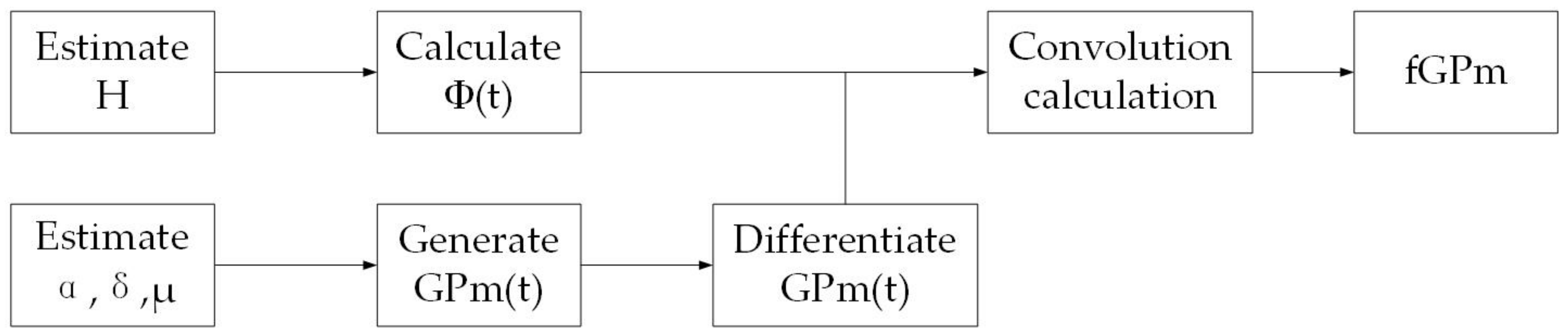
Generalized Pareto motion (GPm) represents the corresponding random process. The fGPm can be constructed by using the GPm to drive the Riemann–Liouville integral.
Note that
as
. Thus, fGPm can be considered as the convolution of the differential of GPm and
.
The flow chart of the generation algorithm is depicted in
Figure 1.
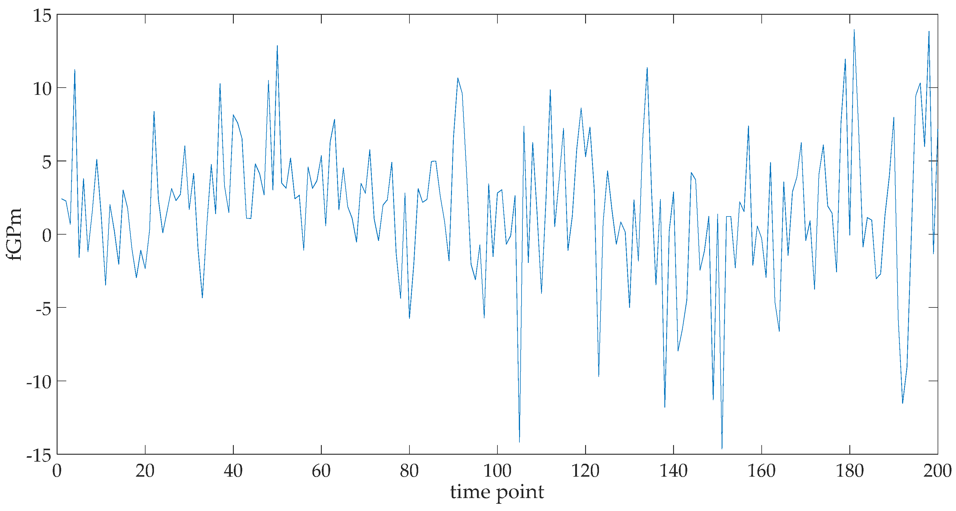
We performed 200 iterations of the fGPm (see
Figure 2). The variance shown represents the measure of the dispersion of the distribution. A previous study [
24] proved that the fGPm has a huge degree of variance, which causes the process to be heavy-tailed. The heavy-tailed characteristics of the fGPm indicate that the simulation path contains frequent long jumps.
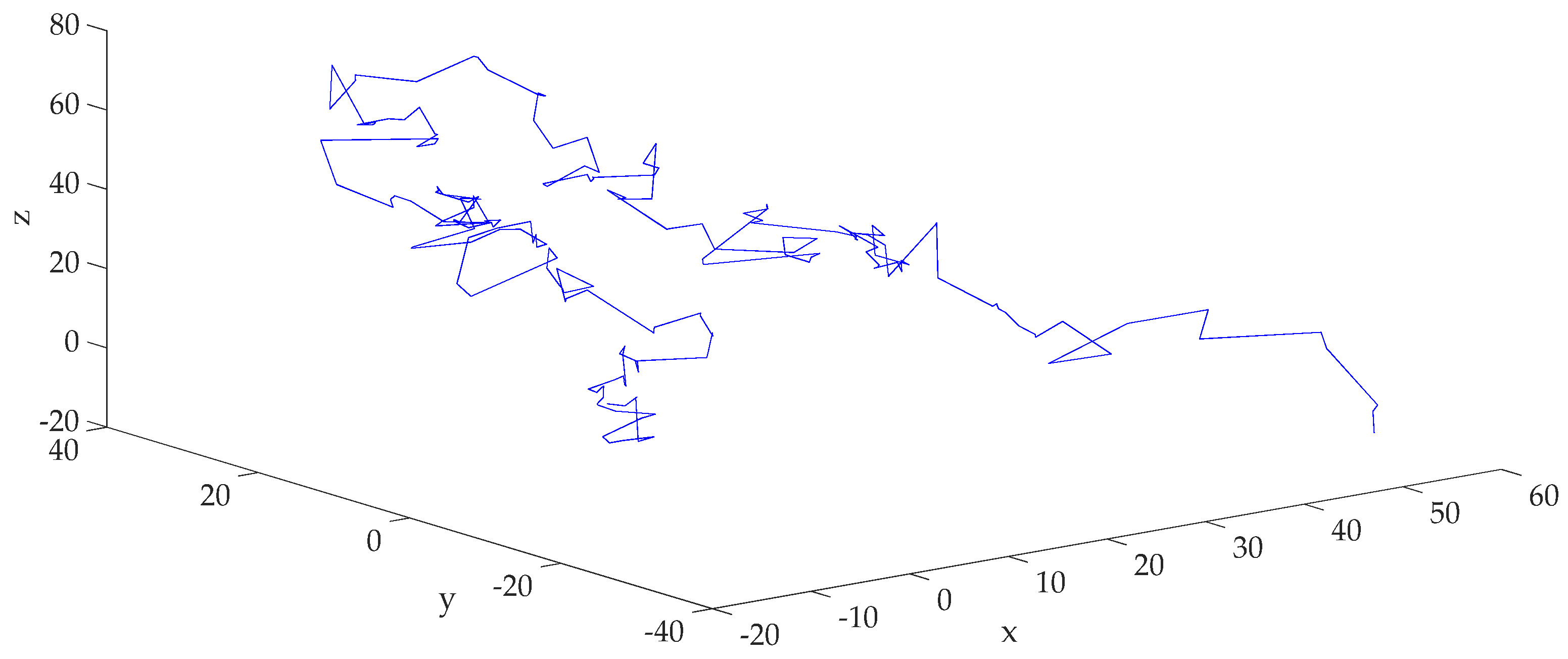
A three-dimensional fGPm random walk with 200 iterations is depicted in
Figure 3. The particle is moving in the three-dimensional space, with the initial position as its origin. In each iteration of the random walk, the moving direction for the particle is random and the jump length is subject to fGpm. For the heavy-tailed stochastic process, the jump lengths are usually long, and the area of movement is vast.
2.2. Long-Range Dependence and Self-Similarity of the fGPm
The parameters in the generalized Pareto distribution have a similar meaning as the Lévy distribution [
29]. When the Hurst exponent, H, of the fractional Lévy stable motion is greater than
, the previous values and successive values are positively related, which ensures the prediction accuracy. Therefore, the fractional Lévy stable motion has long-range dependence for
. Similarly, the long-range dependence of the fGPm also requires that
.
In the stochastic process,
is self-similar if a constant
exists to make the following condition holds true for any constant
:
where
denotes equality in the distribution.
Similar to the Lévy stable motion, the GPm is
and is self-similar:
Note that the fGPm is a self-similar process with the parameter of
, and the derivation is as follows:
2.3. The Difference and Iteration in the fGPm Predictive Model
The difference iterative prediction model is based on the Langevin-type stochastic differential equation (SDE), driven by the fGPm [
30]:
where
and
denote the global trend and volatility rate, respectively.
Note that the increment of the fGPm is not analytical; therefore, we apply the Maruyama notation for the derivation of the predictive model [
31]:
where
is the white noise conforming to a generalized double Pareto distribution [
24]. The location parameter is set to be zero for further derivation and the other parameters are estimated from the actual incremental data.
This provides the facility to combine the discretized forms of Equations (7) and (8):
Therefore, we can conclude the prediction formula for the future values:
Let
be a predictive time frame:
where
is the prediction time point.
This concludes the derivation for the difference iterative prediction model, based on the fGPm. The forecasting process is an additive iteration of the differences between two adjacent time points.
2.4. Parameter Estimation
In order to estimate the parameters for the predictive model, the increments of the dataset are calculated.
The estimation of location parameters is the mean of the incremental data:
In order to estimate the scaling and tail parameters, we use the maximum likelihood estimation, which reads as follows:
Then we take the logarithm to both sides of Equation (13), and we get the following:
Furthermore, the partial derivatives of Equation (14) are taken with respect to the scaling parameter and tail parameter. After elementary transformations, we obtain the following identities:
To estimate parameter
, we define a new quantity,
.
The mean of the white noise is zero, therefore Equation (18) can be established.
Therefore, the estimation of
reads as follows:
In order to calculate parameter
, we introduce a new variable,
, which reads as follows (see Equation (20)):
Then, one can estimate the value of
:
3. Combination of the Hidden Markov Model and Cosine-Similarity
The core of the hidden Markov model lies in the directed graph. Any state variable that is not observed directly is called a hidden variable. As time passes, the system switches among different states. Each state variable has an observed variable. In the prediction of meteorological quantities, extracting information from historical data is important because the climate in the area is stable. Therefore, cosine similarity is employed for similarity analysis of the solar irradiance within the same time frames (one year). Our CS-HMM model represents a hidden Markov model, in which the feature vector is calculated by using a cosine similarity measure.
Let
V and
W be
n-dimensional vectors; one can visualize the similarity of the two vectors as the cosine of the angle between
V and
W. From a geometric standpoint, the angle between
V and
W is given by:
where
and
are the elements of vectors
and
.
In order to calculate the feature vector, we need to constitute a radiation vector. The values in the vector are the solar radiation for the same day on five consecutive years. Then, the variation of the solar irradiance between two adjacent values in the radiation vector is calculated to form the variation vector. The three-dimensional vectors, named
and
, are defined as follows:
where
are the elements of the variation vector.
The cosine similarity between , , and a common criterion vector, , are calculated.
The elements in the three-dimensional criterion vector are randomly chosen as 0 and 1.
Equation (27) defines the feature vector,
:
For the predictive analysis, we select a value for the training set to be the candidate for prediction. Then, we calculate the feature vector between the candidate and the four last values of the training set. The vector with the maximum probability is preferred, and the corresponding candidate is the predicted value. If we set a prediction length, n, and repeat the process for n times, then the solar radiation prediction, based on CS-HMM, is completed.
The nonhomogeneous Markov jump system is suitable for describing the dynamical systems when subject to random changes [
32]. In solar irradiation prediction, the disturbance in the system is subject to the historical data and meteorological conditions. Therefore, it is more appropriate to employ a cosine similarity to extract historical information. The Takagi–Sugeno fuzzy model and singular system theory are not applied in this research, due to the excess computational complexity involved [
33,
34].
4. Hybrid Algorithm, Based on fGPm and CS-HMM
4.1. Calculation for the Number of Prediction Steps
To begin the hybrid prediction, the MPS must be determined. Within the MPS, the accuracy of the prediction can be secured. The MPS is the reciprocal of the maximum Lyapunov exponent, which is obtained via the small-data method [
26]:
where max
Ly is the maximum Lyapunov exponent.
4.2. Hybrid Predictive Algorithm
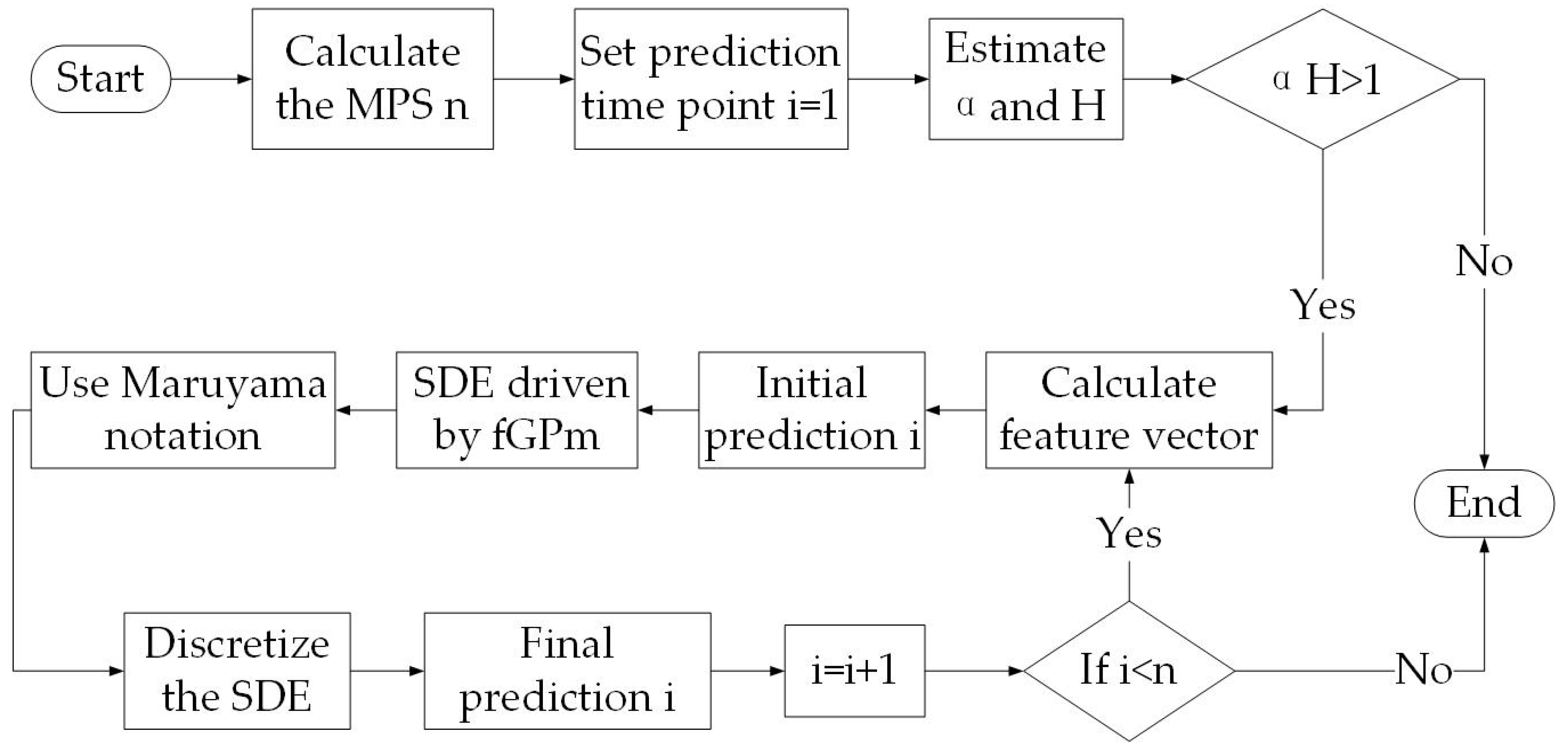
In this paper, the predictions based on statistical properties and artificial intelligence are combined to form a hybrid prediction model. Both the statistical characteristics and the training of historical data are utilized. The hybrid algorithm, which is based on fGPm and CS-HMM, can be divided into six steps:
- (1)
The MPS is obtained by calculating the maximum Lyapunov exponent.
- (2)
The long-range dependence condition for the fGPm difference iterative prediction model is tested.
- (3)
The initial prediction of the solar radiation is carried out, based on the CS-HMM algorithm.
- (4)
The initial prediction results are fed to the SDE, driven by fGPm to predict future increments.
- (5)
The Maruyama notation is employed in the discretized SDE.
- (6)
The prediction is finalized with the difference and iteration.
The flow chart of the prediction is in
Figure 4. The essence of the hybrid algorithm isa two-step prediction. First, the CS-HMM algorithm is utilized to reach the initial prediction results. Second, the initial prediction results are substituted into the SDE for the prediction of increments. The final prediction results are the additive iteration of present values and increments.
5. Case Study
5.1. Dataset of Solar Irradiation
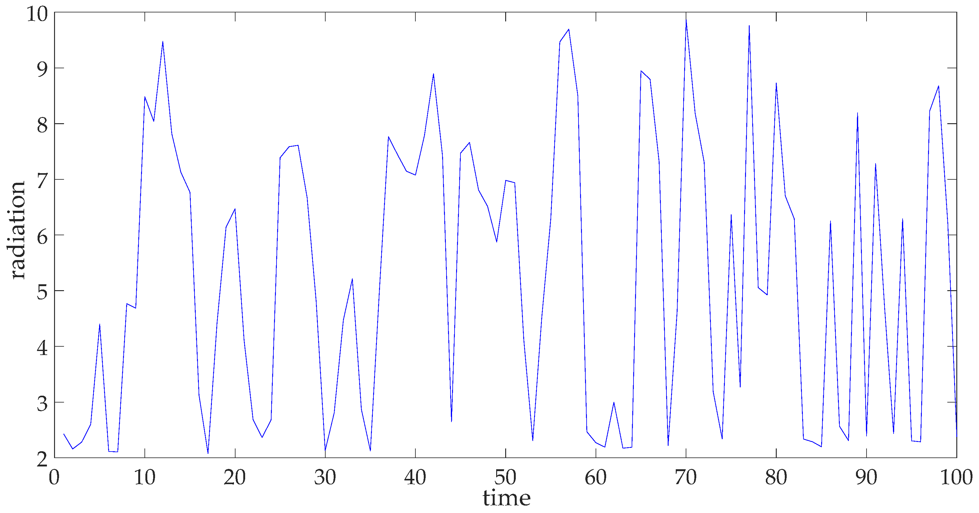
In order to validate our investigation, solar radiation forecasting is performed in the case study. The solar radiation is collected by the meteorological facility in Beijing, which can be found in the
Supplementary Materials. The data for this is collected once a day. The radiation data from 1 July 2014 to 8 October 2014 are used as the training data. The training data are depicted in
Figure 5, in which we can visualize the fluctuation of solar radiation.
As we see from
Figure 5, the fluctuation of the solar irradiance is stationary and periodic. The augmented Dickey–Fuller test is performed using MATLAB, which confirms the stationary nature of the dataset [
35].
5.2. The Number of Prediction Steps for Solar Irradiation Prediction
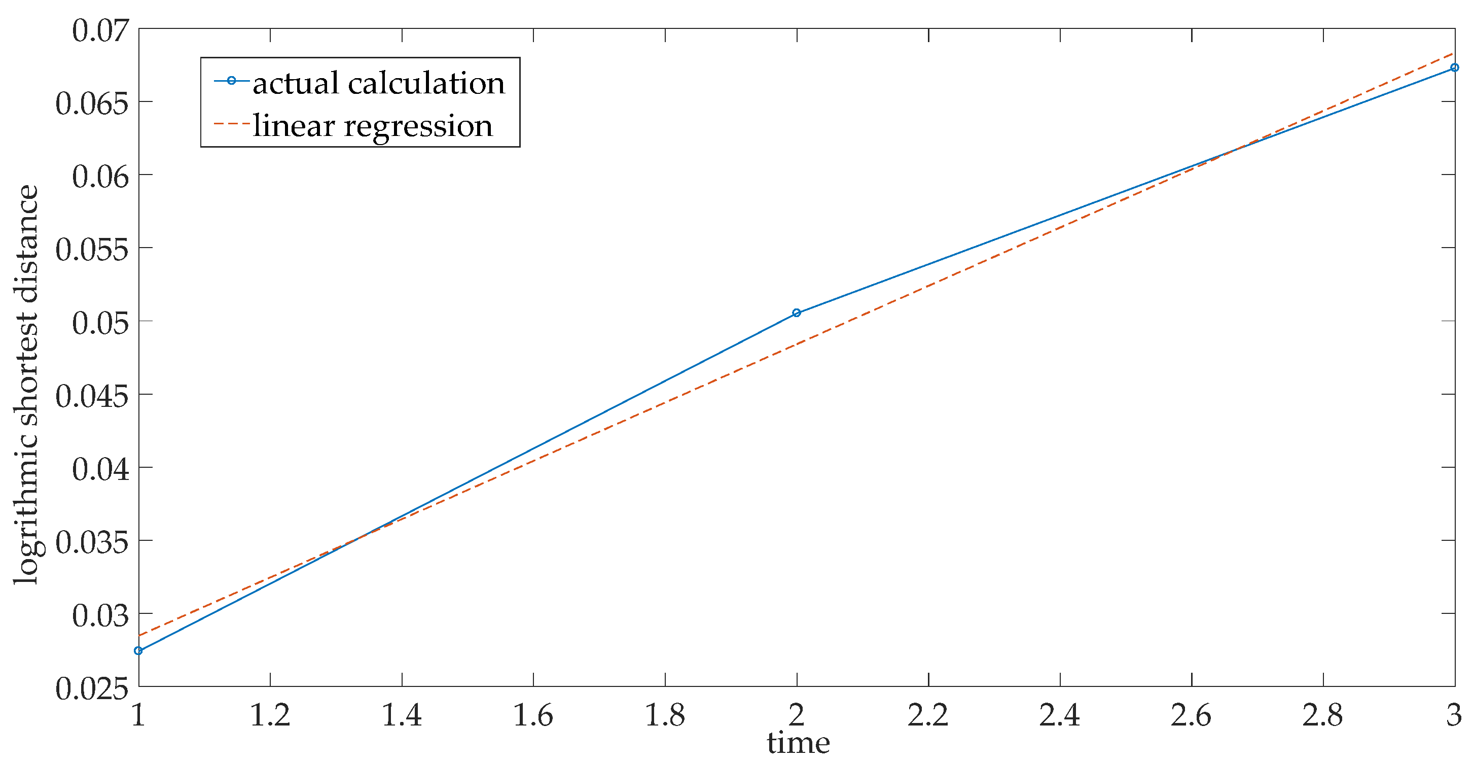
The logarithmic regression is plotted in
Figure 6 for the shortest distance in the reconstructed phase space. As we can see from
Figure 6, the slope of the straight line is the maximum Lyapunov exponent, which is 0.0199. First, we take the integral part of the reciprocal, then we can set the MPS to be 50 time steps.
5.3. Self-Similarity and the Long-Range Dependence of Solar Radiation Prediction
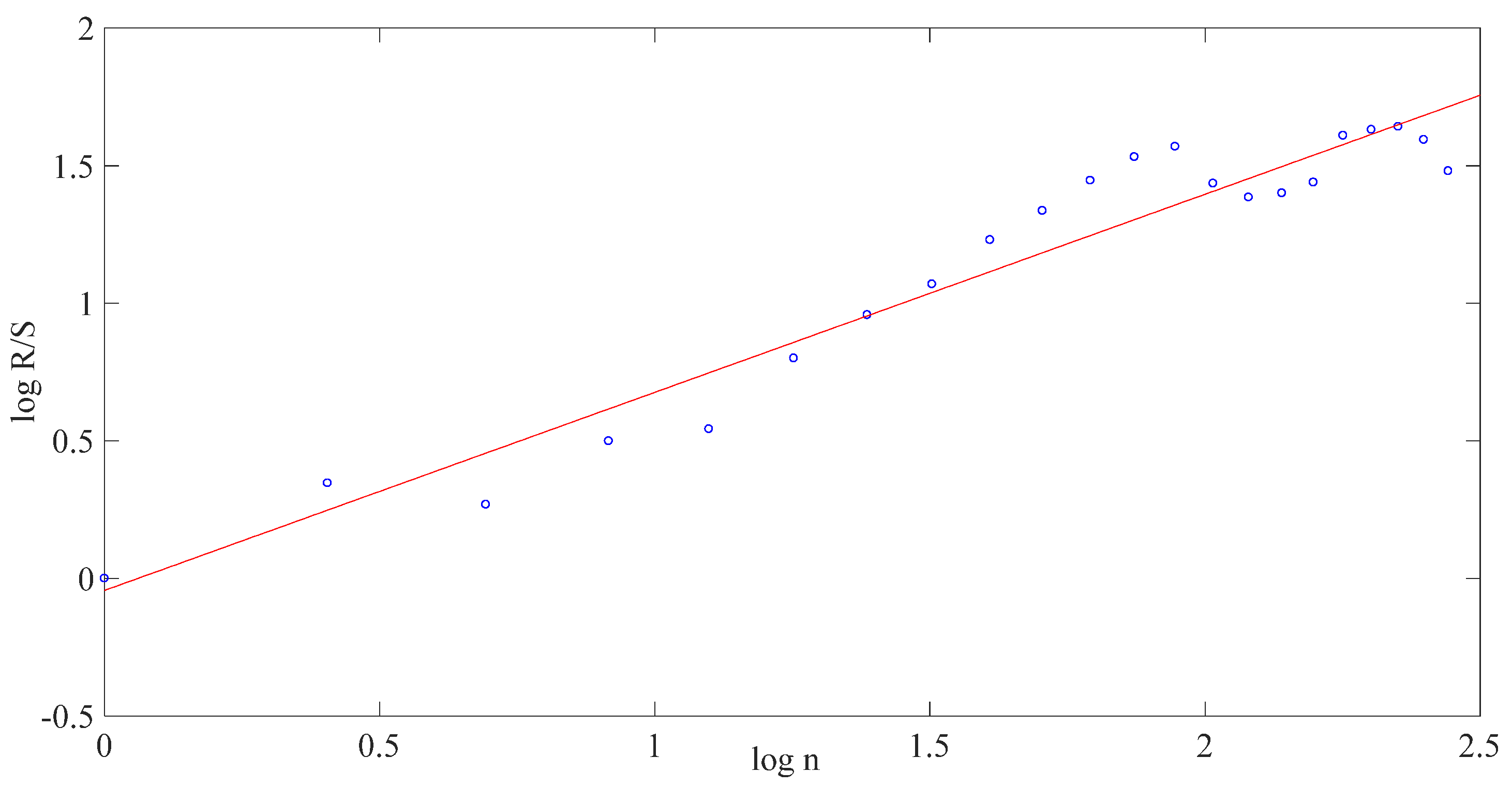
We should recall that the condition for long-range dependence is the following: . We must validate the estimated Hurst and tail parameters to ensure that they satisfy the criterion.
The Hurst exponent was calculated as the slope of the straight line (see
Figure 7). An estimation of the Hurst exponent, evaluated by the R/S method, gives 0.7198. The value of the Hurst exponent verifies the long-range dependence and self-similarity of the data.
The calculated tail parameter, , takes the value of 1.9708. The product between the Hurst exponent and the tail parameter is greater than 1, which shows that the model has long-range dependence.
5.4. Evaluation of the Hybrid Predictive Model
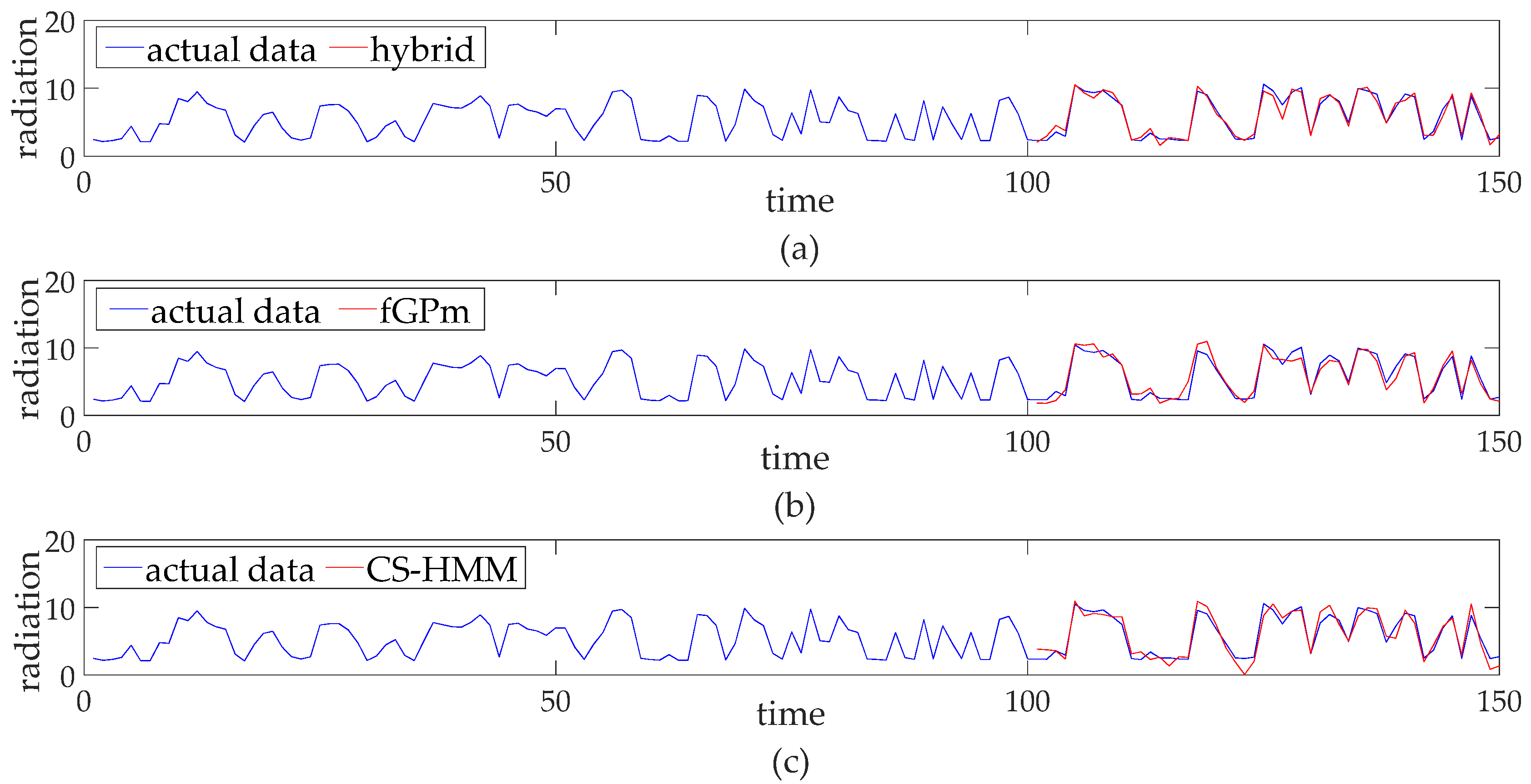
Prediction of solar irradiance was carried out with the hybrid algorithm, the fGPm difference iterative prediction model, and the CS-HMM algorithm. The prediction results are summarized in
Figure 8. The evaluation criteria were calculated for three predictive models, as shown in
Table 1. The mean absolute error (MAE) and the root mean squared error (RMSE) are given by the following formulas:
where
is the ith value of the prediction and
is the
ith value of the actual data.
5.5. Discussion and Future Work
It can be inferred from
Table 1 that the hybrid predictive algorithm shows better performance than the other two methods. The CS-HMM does not take into account the long-range dependence and self-similarity of the data. The disadvantage of the fGPm predictive method is as follows: the current increment is predicted on the basis of the present prediction. The prediction error can be propagated and enlarged during the prediction process. In the hybrid algorithm, long-range dependence and the self-similarity of solar radiation are considered. The error propagation is stopped by utilizing the initial prediction of CS-HMM to form the increment prediction.
Our further investigations will be aimed at an extension of the predictive model. The power load series is chaotic; therefore, the MPS needs to be calculated [
36]. The power load series is long-range-dependent and self-similar [
37,
38]. As reported in an earlier study [
39], the historical data can be used for the prediction of power load. Therefore, the hybrid predictive model can be extended to power load prediction.
6. Conclusions
In this study, we have suggested a hybrid predictive method that is based on the fGPm and CS-HMM models. Self-similarity and the long-range dependence of the fGPm are proven. The CS-HMM employs cosine similarity to extract information from the historical variation. In the hybrid algorithm, the MPS is determined with the maximum Lyapunov exponent. The initial prediction is performed by the CS-HMM and is then substituted into the fGPm difference iterative model to predict the successive values. The hybrid algorithm was then verified, using the dataset of solar irradiance.
The hybrid method utilizes the statistical properties of the dataset and avoids error propagation. The method’s predictive accuracy can be improved if the initial predictive algorithm is optimized.
Author Contributions
Conceptualization, W.S. and D.C.; methodology, W.S. and D.C.; software, W.D., validation, W.S. and A.K.; formal analysis, W.S.; investigation, R.J.; resources, W.S. and A.K.; data curation, W.S. and A.K.; writing—original draft preparation, W.D.; writing—review and editing, D.C.; visualization, R.J.; supervision, W.S.; project administration, W.S.; funding acquisition, W.S. All authors have read and agreed to the published version of the manuscript.
Funding
This research was supported as a major project of the Ministry of Science and Technology of the People’s Republic of China, grant number: 2020AAA0109301.
Institutional Review Board Statement
Not applicable.
Informed Consent Statement
Not applicable.
Data Availability Statement
Acknowledgments
Without the experimental support of the Shanghai University of Engineering Science, Jiangxi New Energy Technology Institute, and the Minnan University of Science and Technology, the research work in this paper could not have been completed.
Conflicts of Interest
The authors declare no conflict of interest.
Abbreviations
| CS-HMM | cosine similarity hidden Markov model |
| fGPm | fractional generalized Pareto motion |
| GPm | generalized Pareto motion |
| SDE | stochastic differentiate equation |
| MPS | maximum prediction steps |
| RMSE | root mean square error |
| MAE | mean absolute error |
| R/S | rescaled range method |
References
- Wu, J.; Chan, C.K. Prediction of hourly solar radiation with multi-model framework. Energy Convers. Manag. 2013, 76, 347–355. [Google Scholar] [CrossRef]
- Ghosh, O.; Chatterjee, T.N. On the Signature of Chaotic Dynamics in 10.7 cm Daily Solar Radio Flux. Sol. Phys. 2015, 290, 3319–3330. [Google Scholar] [CrossRef]
- Debbouche, N.; Almatroud, A.O.; Ouannas, A.; Batiha, I.M. Chaos and coexisting attractors in glucose-insulin regulatory system with incommensurate fractional-order derivatives. Chaos Solitons Fractals 2021, 143, 110575. [Google Scholar] [CrossRef]
- Liu, H.; Song, W.; Zhang, Y.; Kudreyko, A. Generalized Cauchy Degradation Model with Long-Range Dependence and Maximum Lyapunov Exponent for Remaining Useful Life. IEEE Trans. Instrum. Meas. 2021, 702021, 9369345. [Google Scholar] [CrossRef]
- Fainberg, J.; Osherovich, V. Spectroscopy of Electric-Field Oscillations in the Solar Wind During the Passage of a Type III Radio Burst Using Observations Compared with Self-Similar Theory. Sol. Phys. 2022, 297, 50. [Google Scholar] [CrossRef]
- Vipindas, V.; Gopinath, S.; Girish, T.E. A study on the variations in long-range dependence of solar energetic particles during different solar cycles. In Proceedings of the International Astronomical Union, Vienna, Austria, 20–31 August 2018. [Google Scholar] [CrossRef]
- Feng, S.; Wang, X.; Sun, H.; Zhang, Y.; Li, L. A better understanding of long range temporal dependence of traffic flow time series. Phys. A Stat. Mech. Its Appl. 2018, 492, 639–650. [Google Scholar] [CrossRef]
- Zaliapin, I.; Kovchegov, Y. Tokunaga and Horton self-similarity for level set trees of Markov chains. Chaos Solitons Fractals 2012, 45, 358–372. [Google Scholar] [CrossRef] [Green Version]
- Wang, S.Y.; Qiu, J.; Li, F.F. Hybrid Decomposition-Reconfiguration Models for Long-Term Solar Radiation Prediction Only Using Historical Radiation Records. Energies 2018, 11, 1376. [Google Scholar] [CrossRef] [Green Version]
- Narvaez, G.; Giraldo, L.F.; Bressan, M.; Pantoja, A. Machine learning for site-adaptation and solar radiation forecasting. Renew. Energy 2021, 167, 333–342. [Google Scholar] [CrossRef]
- Salcedo-Sanz, S.; Casanova-Mateo, C.; Muñoz-Marí, J.; Camps-Valls, G. Prediction of Daily Global Solar Irradiation Using Temporal Gaussian Processes. IEEE Geosci. Remote Sens. Lett. 2014, 11, 1936–1940. [Google Scholar] [CrossRef]
- Qazi, A.; Fayaz, H.; Wadi, A.; Raj, R.G.; Rahim, N.A.; Khan, W.A. The artificial neural network for solar radiation prediction and designing solar systems: A systematic literature review. J. Clean. Prod. 2015, 104, 1–12. [Google Scholar] [CrossRef]
- Song, W.; Liu, H.; Zio, E. Long-range dependence and heavy tail characteristics for remaining useful life prediction in rolling bearing degradation. Appl. Math. Model. 2022, 102, 268–284. [Google Scholar] [CrossRef]
- Kuhe, A.; Achirgbenda, V.T.; Agada, M. Global solar radiation prediction for Makurdi, Nigeria, using neural networks ensemble. Energy Sources Part A Recovery Util. Environ. Eff. 2021, 43, 1373–1385. [Google Scholar] [CrossRef]
- Capizzi, G.; Napoli, C.; Bonanno, F. Innovative Second-Generation Wavelets Construction With Recurrent Neural Networks for Solar Radiation Forecasting. IEEE Trans. Neural Netw. Learn. Syst. 2012, 23, 1805–1815. [Google Scholar] [CrossRef] [Green Version]
- Dong, N.; Chang, J.F.; Wu, A.G.; Gao, Z.K. A novel convolutional neural network framework based solar irradiance prediction method. Int. J. Electr. Power Energy Syst. 2019, 114, 105411. [Google Scholar] [CrossRef]
- Wang, Z.; Tian, C.; Zhu, Q.; Huang, M. Hourly Solar Radiation Forecasting Using a Volterra-Least Squares Support Vector Machine Model Combined with Signal Decomposition. Energies 2018, 11, 68. [Google Scholar] [CrossRef] [Green Version]
- Bhardwaj, S.; Sharma, V.; Srivastava, S.; Sastry, O.S.; Bandyopadhyay, B.; Chandel, S.S.; Gupta, J.R.P. Estimation of solar radiation using a combination of Hidden Markov Model and generalized Fuzzy model. Sol. Energy 2013, 93, 43–54. [Google Scholar] [CrossRef]
- Khreich, W.; Granger, E.; Miri, A.; Sabourin, R. On the memory complexity of the forward-backward algorithm. Pattern Recognit. Lett. 2010, 31, 91–99. [Google Scholar] [CrossRef]
- Benyacoub, B.; ElBernoussi, S.; Zoglat, A.; Ouzineb, M. Credit Scoring Model Based on HMM/Baum-Welch Method. Comput. Econ. 2021, 59, 1135–1154. [Google Scholar] [CrossRef]
- Zhou, Y.; Liu, Y.; Wang, D.; De, G.; Li, Y.; Liu, X.; Wang, Y. A novel combined multi-task learning and Gaussian process regression model for the prediction of multi-timescale and multi-component of solar radiation. J. Clean. Prod. 2021, 284, 124710. [Google Scholar] [CrossRef]
- Ayodele, T.R.; Ogunjuyigbe, A.S.O. Prediction of monthly average global solar radiation based on statistical distribution of clearness index. Energy 2015, 90, 1733–1742. [Google Scholar] [CrossRef]
- Fatemi, S.A.; Kuh, A.; Fripp, M. Parametric methods for probabilistic forecasting of solar irradiance. Renew. Energy 2018, 129, 666–676. [Google Scholar] [CrossRef]
- Song, W.; Duan, S.; Chen, D.; Zio, E.; Yan, W.; Cai, F. Finite Iterative Forecasting Model Based on Fractional Generalized Pareto Motion. Fractal Fract. 2022, 6, 471. [Google Scholar] [CrossRef]
- Ghasvarian Jahromi, K.; Gharavian, D.; Mahdiani, H. A novel method for day-ahead solar power prediction based on hidden Markov model and cosine similarity. Soft Comput. 2020, 24, 4991–5004. [Google Scholar] [CrossRef]
- Liu, H.; Song, W.; Zio, E. Generalized Cauchy difference iterative forecasting model for wind speed based on fractal time series. Nonlinear Dyn. 2021, 103, 759–773. [Google Scholar] [CrossRef]
- Castillo, E.; Hadi, A.S. Fitting the Generalized Pareto Distribution to Data. J. Am. Stat. Assoc. 2012, 92, 1609–1620. [Google Scholar] [CrossRef]
- Armagan, A.; Dunson, D.B.; Lee, J. Generalized double Pareto shrinkage. Stat. Sin. 2013, 23, 119–143. [Google Scholar] [CrossRef] [Green Version]
- Penson, K.A.; Górska, K. Exact and Explicit Probability Densities for One-Sided Lévy Stable Distributions. Phys. Rev. Lett. 2010, 105, 210604. [Google Scholar] [CrossRef] [Green Version]
- Kwok, K.Y.; Chiu, M.C.; Wong, H.Y. Demand for longevity securities under relative performance concerns: Stochastic differential games with cointegration. Insur. Math. Econ. 2017, 71, 353–366. [Google Scholar] [CrossRef]
- Leobacher, G.; Szölgyenyi, M. Convergence of the Euler-Maruyama method for multidimensional SDEs with discontinuous drift and degenerate diffusion coefficient. Numer. Math. 2018, 138, 219–239. [Google Scholar] [CrossRef] [Green Version]
- Sathishkumar, M.; Sakthivel, R.; Alzahrani, F.; Kaviarasan, B.; Ren, Y. Mixed H∞ and passivity-based resilient controller for nonhomogeneous Markov jump systems. Nonlinear Anal. Hybrid Syst. 2018, 31, 86–99. [Google Scholar] [CrossRef]
- Sathishkumar, M.; Sakthivel, R.; Kwon, O.M.; Kaviarasan, B. Finite-time mixed H∞ and passive filtering for Takagi–Sugeno fuzzy nonhomogeneous Markovian jump systems. Int. J. Syst. Sci. 2017, 48, 1416–1427. [Google Scholar] [CrossRef]
- Sathishkumar, M.; Sakthivel, R.; Wang, C.; Kaviarasan, B.; Anthoni, S.M. Non-fragile filtering for singular Markovian jump systems with missing measurements. Signal Process. 2017, 142, 125–136. [Google Scholar] [CrossRef]
- Gomez-Biscarri, J.; Hualde, J. A residual-based ADF test for stationary cointegration in I (2) settings. J. Econom. 2015, 184, 280–294. [Google Scholar] [CrossRef]
- Liu, Y.; Lei, S.; Sun, C.; Zhou, Q.; Ren, H. A multivariate forecasting method for short-term load using chaotic features and RBF neural network. Eur. Trans. Electr. Power 2011, 21, 1376–1391. [Google Scholar] [CrossRef]
- Shalalfeh, L.; Bogdan, P.; Jonckheere, E. Evidence of Long-Range Dependence in Power Grid. In Proceedings of the 2016 IEEE Power & Energy Society General Meeting (PES), Boston, MA, USA, 17–21 July 2016. [Google Scholar] [CrossRef]
- Li, C.; Zhuang, H.; Wang, Q.; Zhou, X. SSLB: Self-Similarity-Based Load Balancing for Large-Scale Fog Computing. Arab. J. Sci. Eng. 2018, 43, 7487–7498. [Google Scholar] [CrossRef]
- Lai, C.S.; Mo, Z.; Wang, T.; Yuan, H.; Ng, W.W.; Lai, L.L. Load forecasting based on deep neural network and historical data augmentation. IET Gener. Transm. Distrib. 2020, 14, 5927–5934. [Google Scholar] [CrossRef]
| Disclaimer/Publisher’s Note: The statements, opinions and data contained in all publications are solely those of the individual author(s) and contributor(s) and not of MDPI and/or the editor(s). MDPI and/or the editor(s) disclaim responsibility for any injury to people or property resulting from any ideas, methods, instructions or products referred to in the content. |
© 2023 by the authors. Licensee MDPI, Basel, Switzerland. This article is an open access article distributed under the terms and conditions of the Creative Commons Attribution (CC BY) license (https://creativecommons.org/licenses/by/4.0/).


