Article

A Fast Computational Scheme for Solving the Temporal-Fractional Black–Scholes Partial Differential Equation

1
Department of Mathematics, Hamedan Branch, Islamic Azad University, Hamedan, Iran
2
Mathematical Modeling and Applied Computation (MMAC) Research Group, Department of Mathematics, King Abdulaziz University, Jeddah 21589, Saudi Arabia
3
Department of Mathematics and Applied Mathematics, School of Mathematical and Natural Sciences, University of Venda, P. Bag X5050, Thohoyandou 0950, South Africa
*
Authors to whom correspondence should be addressed.
Fractal Fract. 2023, 7(4), 323; https://doi.org/10.3390/fractalfract7040323
Submission received: 13 March 2023 / Revised: 29 March 2023 / Accepted: 6 April 2023 / Published: 12 April 2023

Abstract

:
In this work, we propose a fast scheme based on higher order discretizations on graded meshes for resolving the temporal-fractional partial differential equation (PDE), which benefits the memory feature of fractional calculus. To avoid excessively increasing the number of discretization points, such as the standard finite difference or meshfree methods, and, at the same time, to increase the efficiency of the solver, we employ discretizations on spatially non-uniform meshes with an attention on the non-smoothness area of the underlying asset. Therefore, the PDE problem is transformed to a linear system of algebraic equations. We perform numerical simulations to observe and check the behavior of the presented scheme in contrast to the existing methods.

1. Introduction

1.1. PDE Formulation

Many of the new practical problems in the literature [1,2] require the derivative not to be of integer order and, due to this, fractional differentiation in several senses in terms of definition must be dealt with in order to model the problems.
Let us assume that a derivative is to be defined by the (right) modified Riemann–Liouville (RL) notion. Then the fractional Black–Scholes (BS) price of an option u, by considering T > 0 as the maturity time, can be written as follows (forward in time) [1,2]:
α u ( z , t ) t α = 1 2 σ 2 z 2 2 u ( z , t ) z 2 + ( r q ) z u ( z , t ) z r u ( z , t ) , z 0 ,
where the interest rate is r and 0 < α 1 . Moreover, α = 2 H , is the real-valued Hurst exponent and 1 > H > 0 , which describes an exponent for the time series’s memory [3]. Clearly (1) will be simplified to the classic BS partial differential equation (PDE) by assuming H = 1 / 2 . Additionally, σ and q are some positive constants. u is deterministic and stands for the fractional option price in an equity market.
For most settings under (1), we must solve numerically the PDE problem to the present and then find the present value of the financial derivative. Time-fractional financial PDEs describe models which have important applications in memory behaviors of long-time heavy tail decay for computational finance. This raises a need for fractional PDE problems and subsequently finding new effective methods are necessary.

1.2. Initial Conditions

The initial condition for the fractional BS option pricing problem (1) is written for the two common cases of put and call as follows (respectively) ([4] Chapter 1):
u ( z , 0 ) = ( K z ) + ,
and
u ( z , 0 ) = ( z K ) + ,
where K stands for the strike price.

1.3. Boundary Conditions

For the put and call cases, the side conditions can be given by, respectively, [5]:
lim z u ( z , t ) = 0 , u ( 0 , t ) = K exp { r t } ,
lim z u ( z , t ) = z max exp ( q t ) K exp ( r t ) , u ( 0 , t ) = 0 ,
where z max is a large fixed constant.

1.4. Caputo Fractional Derivative

For the real continuous function g, the modified Riemann–Liouville (RL) fractional derivative in the fractional calculus can be defined as [6]:
g ( α ) ( t ) : = d α g ( t ) d t α = ( Γ ( α ) ) 1 0 t ( t ζ ) α 1 ( g ( 0 ) + g ( ζ ) ) d ζ , α < 0 , ( Γ ( α + 1 ) ) 1 d d t 0 t ( t ζ ) α ( g ( 0 ) + g ( ζ ) ) d ζ , 0 < α < 1 , d o ( g ( α o ) ( t ) ) d t o , o α < o + 1 ,
where Γ ( · ) is the Gamma function and o is a constant. Recall that fractional differentiation in the Caputo sense is given as follows [7]:
0 C D t α g ( t ) = 0 t ( t ζ ) α g ( ζ ) d ζ ( Γ ( 1 α ) ) 1 , 0 < α < 1 .

1.5. Time Discretization

Let the time discretization be given as 0 = t 0 < t 1 < < t n = T , with the equally-spaced step size Δ t also given. The author in [8] presented the L1 scheme for computing the RL fractional differentiation on the function g as follows:
0 R D t α ( g ( t n ) ) = Δ t α j = 0 n f j , n g ( t n j ) + O ( Δ t α + 2 ) ,
wherein
Γ ( α + 2 ) f j , n = ( j 1 ) α + 1 j α + 1 , j = n , ( 1 + j ) α + 1 + ( j + 1 ) α + 1 2 j α + 1 , 1 j n 1 , 1 , j = 0 .
For equally-spaced stencils, the L1 scheme can also be written in the form below:
0 C D t α ( u ( z i , t k + 1 ) ) = Δ t α Γ [ 2 α ] j = 0 k u i , j + 1 u i , j Δ t ( j ) 1 α + ( 1 + j ) 1 α .

1.6. Background on Numerical Methods

Numerical methods for PDEs are necessary for challenging PDEs arising in real applications. Mostly, methods are constructed belonging to various categories such as finite differences (FD) and finite element methods (FEMs). FD methods discussed for such problems mainly in [9,10,11]. The meshfree RBF methods based on a shape parameter were also discussed for resolving (1) very recently in [12].
It is commented that it is possible to first impose a logarithmic transformation on (1) to obtain a PDE formulation which does not have variable coefficients anymore. However, this is not done here since this transformation encounters the logarithm of zero and an unbounded domain on two sides, which is harder to deal with than the original one which has unboundedness only from one side.
The main target of the present investigation is to follow the works [13,14,15] and propose a fast and efficient scheme for solving (1) but with an employment of graded meshes. The motivation behind choosing graded meshes is that the original fractional PDE problem has non-smoothness at the strike price and thus a non-uniform discretization of higher order will help improving the accuracy of the numerical results. The main motivation behind the designed numerical method is to have a fourth-order method for spatial discretization with an adaptation on the financial hot area of the problem. In fact, a main drawback in the already published works to tackle (1) is that they rely on second-order approximations on uniform meshes which can result in losing some accuracies for low number of discretization points specially around the strike price ( z = K ).

1.7. Paper’s Outline

The remaining parts of this manuscript are as follows. Section 2 provides a graded mesh, i.e., a nonuniform mesh that we need to discretize (1)–(3) adaptively with a clear focus on the financially significant area, at which the underlying asset tends to z = K . Section 3 describes a high-order discretization along the spatial variable of fourth order by employing five/six adjacent nodes since the fourth order must attain on a graded mesh. Section 4 investigates how the proposed solver can be constructed in sparse arrays and matrix forms as elegantly as possible. Section 5 is devoted to the numerical investigation of our high-order solver. Numerical experiments are given and discussed in detail therein. A summary of the work is furnished in Section 6.

2. Spatial Discretization Nodes

Numerical solution methods generally utilize the discretization methord to perform approximate calculations. When the interval is partitioned more finely, the calculation result is closer to the theoretical solution. To proceed, we first recall an algorithm to produce adaptive meshes with an emphasis on the non-smooth part of the initial condition. This is pursued by employing the inverse of hyperbolic function which and mapping some sets of points based on such function to have more number of discretization nodes on the hot area. Then, we construct the fourth-order FD approximations on these meshes using five adjacent nodes for estimating the first derivative and six adjacent nodes in computing the second derivative of a function.
We now assume that { z i } i = 1 m is a partition for z [ z min , z max ] . Now, a well-resulted mesh can be given as follows [16]:
z i = Ψ ( μ i ) , i = 1 , 2 , , m ,
where m 3 and
μ max = μ m > > μ 2 > μ 1 = μ min ,
are m equidistant nodes and we also use:
μ int = z right z left d 1 , μ min = sinh 1 z min z left d 1 , μ max = μ int + sinh 1 z max z right d 1 .
We too take into account that z min = 0 and z max = 3 K . The parameter υ 1 > 0 controls the node density around z = K . In addition, one defines
Ψ ( μ ) = z left + υ 1 sinh ( μ ) , μ min μ < 0 , z left + υ 1 μ , 0 μ μ int , z right + υ 1 sinh ( μ μ int ) , μ int < μ μ max .
The idea behind the definition of Ψ ( μ ) is to use hyperbolic functions in order to stretch the points. Using such a function and its application as a zooming function, we can stretch the discretization points. Here in (13), we consider υ 1 = K 20 , while z left = max { e 0.0025 T , 0.5 } × K , z right = K , and [ z left , z right ] [ 0 , z max ] ,16].

3. A Fast High-Order Discretization

Let us consider the graded mesh (14) along the spatial independent variable of the PDE problem. To derive and introduce FD approximation on such graded meshes, five and six stencil nodes must be taken into account at each position of the computational discretized domain to finally attain approximated FD formulas which are of higher order of convergence, four, for both the first and second derivatives of the function.
Accordingly, without loss of generality, we take into consideration that g ( z ) is a sufficiently differentiable function and there is a given set of discretized points as follows:
{ z 1 , z 2 , , z m 1 , z m } .
Here (15) is an arbitrary discretization of points and thus is it a graded mesh. In practice, it is produced by (11)–(14). Now five nodal points are considered as follows:
{ { z i 2 , g ( z i 2 ) } , { z i 1 , g ( z i 1 ) } , { z i , g ( z i ) } , { z i + 1 , g ( z i + 1 ) } , { z i + 2 , g ( z i + 2 ) } } ,
and we calculate the interpolatory polynomial passing through the adjacent points; see e.g., [17]. By employing z = z i and some symbolic computations, one obtains the following FD formulation on our graded mesh:
g ( z i ) = a i 2 g z i 2 + a i 1 g z i 1 + a i g z i + a i + 1 g z i + 1 + a i + 2 g z i + 2 + O h 4 ,
wherein the maximum spacing of local grid is h. Finally we attain
a i 2 = ϱ i 1 , i ϱ i , i + 1 ϱ i , i + 2 ϱ i 2 , i 1 ϱ i 2 , i ϱ i 2 , i + 1 ϱ i 2 , i + 2 ,
a i 1 = ϱ i 2 , i ϱ i , i + 1 ϱ i , i + 2 ϱ i 2 , i 1 ϱ i 1 , i ϱ i 1 , i + 1 ϱ i 1 , i + 2 ,
a i = 1 ϱ i 2 , i ϱ i , i 1 ϱ i , i + 1 ϱ i , i + 2 Z 1 ,
a i + 1 = ϱ i 2 , i ϱ i , i 1 ϱ i , i + 2 ϱ i 2 , i + 1 ϱ i + 1 , i 1 ϱ i + 1 , i ϱ i + 1 , i + 2 ,
a i + 2 = ϱ i 2 , i ϱ i , i 1 ϱ i , i + 1 ϱ i 2 , i + 2 ϱ i + 2 , i 1 ϱ i + 2 , i ϱ i + 2 , i + 1 ,
using ϱ l , q = z l z q and
Z 1 = z i 2 ( z i 1 ( ϱ i + 1 , i + ϱ i + 2 , i ) + 3 z i 2 2 ( z i + 2 + z i + 1 ) z i + z i + 1 z i + 2 ) + z i ( 4 z i 2 + 3 ( z i + 1 + z i + 2 ) z i 2 z i + 1 z i + 2 ) + z i 1 ( 3 z i 2 2 ( z i + 2 + z i + 1 ) z i + z i + 1 z i + 2 ) .
The FD formulations (of the sided type) must be derived similarly and employed for the points on the boundaries and only the one near to the boundaries to have a unified fourth order of convergence. It is noted that, in the case of applying these formulas on structured grids, the fourth order of convergence is preserved.
Using a similar approach, we may obtain the weighting coefficients for approximating the 2nd derivative of the function using graded meshes and having fourth order of convergence. Hence, it is considered that:
{ { z i 3 , g ( z i 3 ) } , { z i 2 , g ( z i 2 ) } , { z i 1 , g ( z i 1 ) } , { z i , g ( z i ) } , { z i + 1 , g ( z i + 1 ) } , { z i + 2 , g ( z i + 2 ) } } ,
and the 2nd-derivative interpolatory function g ( z ) is calculated based on z. At this moment, by considering z = z i , one obtains [17]:
g ( z i ) = b i 3 g z i 3 + b i 2 g z i 2 + b i 1 g z i 1 + b i g z i + b i + 1 g z i + 1 + b i + 2 g z i + 2 + O h 4 ,
wherein
b i 3 = Z 2 ϱ i 3 , i 2 ϱ i 3 , i 1 ϱ i 3 , i ϱ i 3 , i + 1 ϱ i 3 , i + 2 ,
b i 2 = Z 3 ϱ i 3 , i 2 ϱ i 2 , i 1 ϱ i 2 , i ϱ i 2 , i + 1 ϱ i 2 , i + 2 ,
b i 1 = Z 4 ϱ i 2 , i 1 ϱ i 1 , i 3 ϱ i 1 , i ϱ i 1 , i + 1 ϱ i 1 , i + 2 ,
b i = Z 5 ϱ i 3 , i ϱ i , i 2 ϱ i , i 1 ϱ i , i + 1 ϱ i , i + 2 ,
b i + 1 = Z 6 ϱ i 3 , i + 1 ϱ i + 1 , i 2 ϱ i + 1 , i 1 ϱ i + 1 , i ϱ i + 1 , i + 2 ,
b i + 2 = Z 7 ϱ i 3 , i + 2 ϱ i + 2 , i 2 ϱ i + 2 , i 1 ϱ i + 2 , i ϱ i + 2 , i + 1 .
Here, we obtain
Z 2 = z i 1 ( 6 z i 2 + 4 ( z i + 2 + z i + 1 ) z i 2 z i + 1 z i + 2 ) + 2 z i ( 4 z i 2 3 ( z i + 2 + z i + 1 ) z i + 2 z i + 1 z i + 2 ) + z i 2 ( 6 z i 2 + 4 ( z i + 1 + z i + 2 ) z i 2 z i + 1 z i + 2 + z i 1 ( 4 z i 2 ( z i + 1 + z i + 2 ) ) ) , Z 3 = 2 ( z i 3 ( z i 1 ( ϱ i + 1 , i + ϱ i + 2 , i ) + 3 z i 2 2 ( z i + 1 + z i + 2 ) z i + z i + 1 z i + 2 ) + z i ( 4 z i 2 + 3 ( z i + 1 + z i + 2 ) z i 2 z i + 1 z i + 2 ) + z i 1 ( 3 z i 2 2 ( z i + 1 + z i + 2 ) z i + z i + 1 z i + 2 ) ) , Z 4 = 2 ( z i 3 ( z i 2 ( ϱ i + 1 , i + ϱ i + 2 , i ) + 3 z i 2 2 ( z i + 1 + z i + 2 ) z i + z i + 1 z i + 2 ) + z i ( 4 z i 2 + 3 ( z i + 1 + z i + 2 ) z i 2 z i + 1 z i + 2 ) + z i 2 ( 3 z i 2 2 ( z i + 1 + z i + 2 ) z i + z i + 1 z i + 2 ) ) , Z 5 = 2 ( z i 2 ( z i 1 ( ϱ i + 1 , i + ϱ i + 2 , i z i ) + 6 z i 2 3 ( z i + 1 + z i + 2 ) z i + z i + 1 z i + 2 ) + z i 3 ( z i 1 ( ϱ i + 1 , i + ϱ i + 2 , i z i ) + z i 2 ( ϱ i + 1 , i + ϱ i + 2 , i + z i 1 z i ) + 6 z i 2 3 z i + 1 z i 3 z i + 2 z i + z i + 1 z i + 2 ) + z i ( 2 z i ( 3 z i + 1 5 z i ) + z i 1 ( 6 z i 3 z i + 1 ) ) + ( 3 z i ( 2 z i z i + 1 ) + z i 1 ( z i + 1 3 z i ) ) z i + 2 ) ,
Z 6 = 2 ( z i ( z i 1 ( 2 ϱ i , i + 2 + z i ) + z i ( 3 z i + 2 4 z i ) ) + z i 2 ( z i ( 2 ϱ i , i + 2 + z i ) + z i 1 ( ϱ i + 2 , i z i ) ) + z i 3 ( 2 z i ϱ i , i + 2 + z i 1 ( ϱ i + 2 , i z i ) + z i 2 ( ϱ i 1 , i + ϱ i + 2 , i ) + z i 2 ) ) , Z 7 = 2 ( z i ( z i 1 ( 2 ϱ i , i + 1 + z i ) + z i ( 3 z i + 1 4 z i ) ) + z i 2 ( z i ( 2 ϱ i , i + 1 + z i ) + z i 1 ( ϱ i + 1 , i z i ) ) + z i 3 ( 2 z i ϱ i , i + 1 + z i 1 ( ϱ i + 1 , i z i ) + z i 2 ( ϱ i 1 , i + ϱ i + 1 , i ) + z i 2 ) ) .
Here, in fact, the FD approximation (25) based on Taylor expansions of appropriate orders and severe simplifications were performed on graded meshes. Note that, for the nodes { z 1 , z 2 , z 3 , z m 1 , z m } and to keep the quartical speed, a similar procedure can be performed by the six adjacent nodes as discussed above but for that specific node. The relations (17) and (25) are applicable on both graded and uniform meshes and, in the case of equidistant discretion nodes, can yield in more accurate formulations.

4. Construction of the Solver
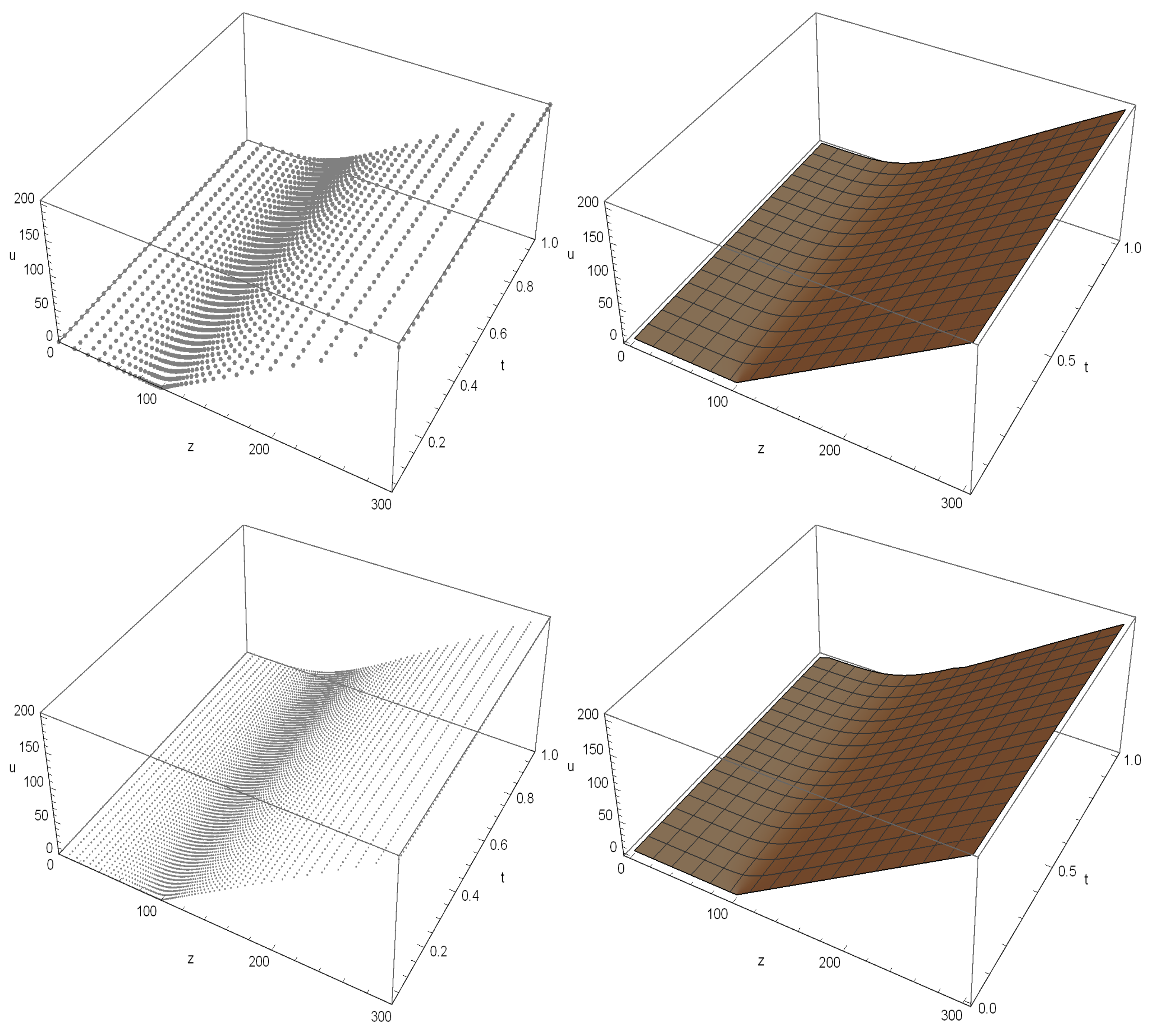
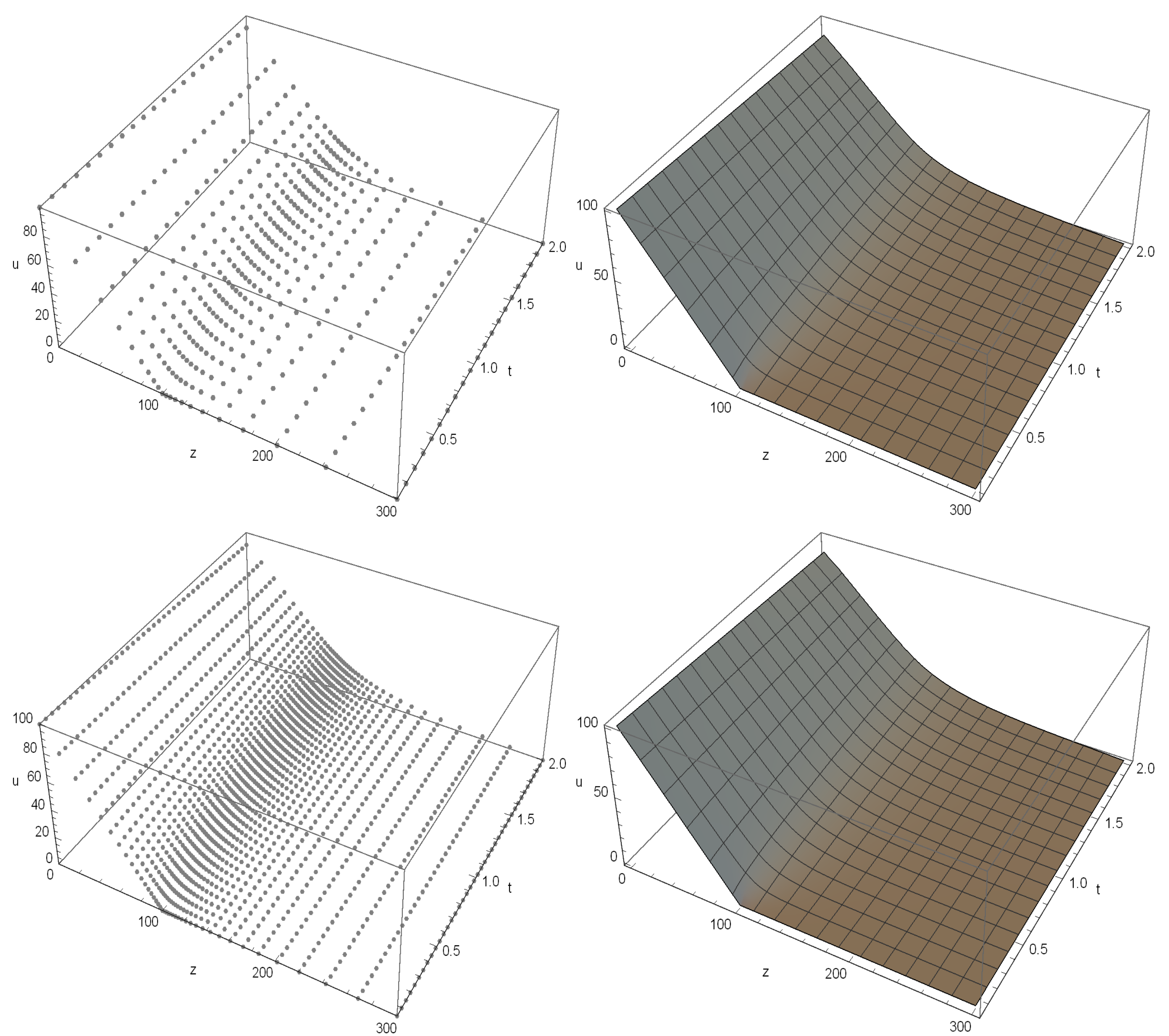
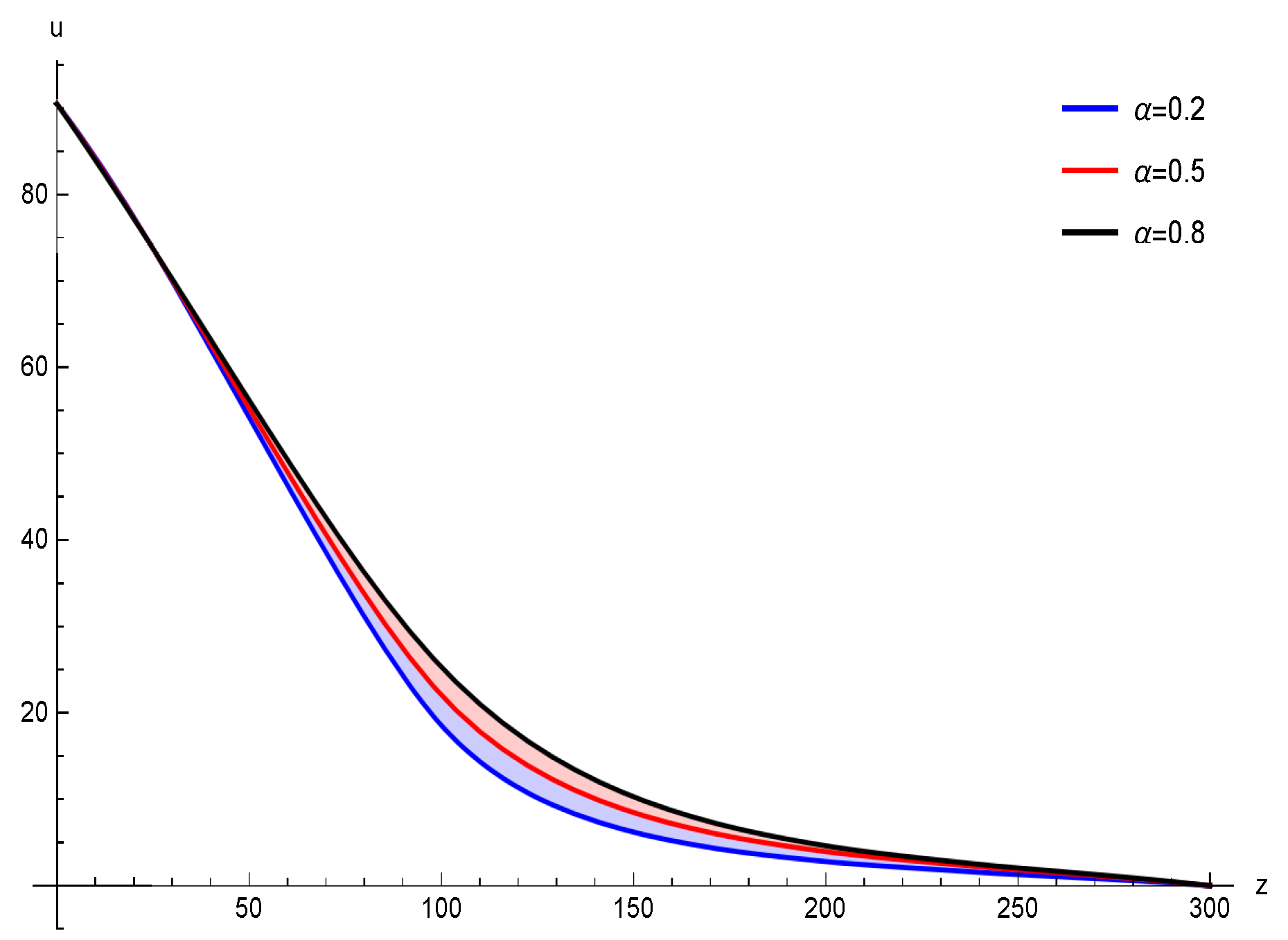
By denoting u i , j u ( z i , t j ) , one can find now the whole discretization solver for (1) as follows:
D t α u ( z i , t j + 1 ) + O ( Δ t 2 α ) = 1 2 σ 2 z i 2 [ b i 3 , j u i 3 , j + b i 2 , j u i 2 , j + b i 1 , j u i 1 , j + b i , j u i , j + b i + 1 , j u i + 1 , j + b i + 2 , j u i + 2 , j ] + O ( h 4 ) + ( r q ) z i [ a i 2 , j u i 2 , j + a i 1 , j u i 1 , j + a i , j u i , j + a i + 1 , j u i + 1 , j + a i + 2 , j u i + 2 , j ] + O ( h 4 ) r u i , j .
It is now possible to write down
D t α u ( z i , t j + 1 ) = Γ [ 2 α ] 1 l = 0 j u i , l + 1 u i , l Δ t l + 1 ( t l + t j + 1 ) 1 α ( t j + 1 t l + 1 ) 1 α .
To continue more formally, now the derivative matrices corresponding to the weights obtained by employing fourth-order approximations in Section 3 are gathered up in some matrices as follows:
M z = a i , j by ( 18 ) i j = 2 , a i , j by ( 19 ) i j = 1 , a i , j by ( 20 ) i j = 0 , a i , j by ( 21 ) j i = 1 , a i , j by ( 22 ) j i = 2 , 0 otherwise ,
and
M z z = b i , j by ( 26 ) i j = 3 , b i , j by ( 27 ) i j = 2 , b i , j by ( 28 ) i j = 1 , b i , j by ( 29 ) i j = 0 , b i , j by ( 30 ) j i = 1 , b i , j by ( 31 ) j i = 2 , 0 otherwise .
We now denote the time derivative matrix as M t . Hence, to derive our proposed method using matrix notations, we consider the following matrix:
Y = 1 2 σ 2 Z 2 ( M z z I t ) + ( r q ) Z ( M z I t ) r I N ,
where ⊗ is the Kronecker product and
Z = diag z 1 , z 2 , , z m I t .
Consider A m × n and B p × q and two matrices, then their Kronecker product C = A B is an ( m p ) × ( n q ) matrix as followss [18]:
c α , β = a i , j b k , l ,
wherein
α = p ( i 1 ) + k , β = q ( j 1 ) + l .
Here I N = I z I t , is an N × N identity matrix, with I z and I t being m × m and n × n identity matrices, respectively. Thus, the temporal-fractional PDE (33) is finally fully discretized as follows:
( I z M t ) U = Υ U ,
where U = ( u 1 , 1 , u 1 , 2 , , u m , n ) * . Now we take into account
B = ( I z M t ) Υ .
Thus, one obtains B U = 0 . By incorporating the boundary and initial conditions, one is able to find a system of linear algebraic equations:
B ¯ U = b ¯ ,
wherein b ¯ and B ¯ are the vector and system matrix, respectively, after incorporating the conditions related to the initial and side.
Based on truncation errors obtained using the approximations used along the spatial and temporal variables of the PDE problem (1), the convergence order is O ( Δ t 2 α ) + O ( h 4 ) . Moreover, the consistency of the solving procedure can be obtained when Δ t , h tend to zero.

5. Numerical Tests

The major point here is to compare and exhibit the efficiency of different schemes to solve (1) on the same numerical domain. The solvers are summarized as follows:
  • The quadratically convergent FD method presented in [19] and shown by FDM.
  • The RBF-FD method on graded meshes given in [20] and denoted by SM.
  • The presented scheme given in this work and shown by PMBS via the non-uniform mesh in Section 3.
Mathematica 12.0 [21] has been used to perform the calculations and write the programs. The computer specifications are Windows 11, Core i7-8750h. Here, z max = 3 K is considered for the numerical domains and the computational time is given in second. Furthermore, the absolute error can be calculated as:
ε = u approx u ref ,
wherein u ref and u approx are the referenced and numerical solutions, respectively.
Example 1.
Let us consider the parameters below for solving (1) in the call case:
α = 0.8 , σ = 40 % , K = 100 $ , q = 0 , T = 1 year , r = 5 % .
The reference value is u ( K , T ) 18.1883 , [20].
Table 1 consists of the convergence history of different solvers. Based on the observations, the proposed high-order method is efficient and gives higher accuracies in lower computational time. Additionally, to check the numerical stability of the presented scheme in practice, the computational solution attained for Example 1 is given in Figure 1 for various numbers of discretization points.
Example 2.
Let us consider the parameters below for solving (1) in the put case:
α = 0.7 , σ = 30 % , q = 20 % , T = 2 year , r = 5 % , K = 100 $ .
The reference solution is taken from [20] as u ( K , T ) 24.6299 .
Numerical pieces of evidence have been furnished in Table 2. They too reveal that the presented scheme converges faster and is more effective for solving the temporal fractional BS PDE. For Example 2, the numerical solutions for various numbers of discretization points are given in Figure 2 as well.
Example 3.
In this test, consider the same assumptions as in Example 2 but different α = { 0.2 , 0.5 , 0.8 } to observe how the numerical solutions behave.
This is pursued by imposing the proposed high-order procedure of this work with 21 discretization points, which is 20 un-equally spaced discretized nodes. The nodes are obtained via (11). The numerical observations are gathered in Figure 3. It is revealed that by increasing α the price of the option increases especially on the hotzone (around the strike price).

6. Conclusions

One of the fundamental and important problems in mathematical finance is to price options via the PDE of BS. Several extensions to this model were given in the literature, such as the model of Heston. However extensions based on the fractional Brownian motion which leads to fractional BS PDE are of practical importance since the memory feature of fractional derivatives can help obtain more reliable option prices in equity markets. To achieve this goal, we have proposed a high-order discretization scheme for solving the fractional BS PDE using graded meshes, i.e., on non-uniform meshes. The motivation of using this was to concentrate more on the hotzone. In this area, the initial condition has a payoff. We have presented our solver on sparse matrices and by the help of the Kronecker product, we have transformed the whole PDE into a system of algebraic linear equations. Numerical tests have been carried out and confirmed the superiority of the novel high-order method for solving fractional BS PDE. Table 1 and Table 2 show the convergence history of different solvers while revealing that our proposed solver is better than the FDM and the SM schemes. Forthcoming studies can be focused on the use of graded meshes on rough Heston PDE along with high-order discretizations to propose a fast solver for such a problem.

Author Contributions

Conceptualization, R.G., T.L., M.Z.U.; formal analysis, T.L., M.Z.U. and S.S.; funding acquisition, R.G., T.L., S.S.; investigation, M.Z.U. and S.S.; methodology, R.G., T.L., M.Z.U.; supervision, R.G., T.L.; validation, M.Z.U., S.S.; writing—original draft, R.G. and S.S.; writing—review & editing, M.Z.U. and S.S. All authors have read and agreed to the published version of the manuscript.

Funding

This research received no external funding.

Institutional Review Board Statement

Not applicable.

Informed Consent Statement

Not applicable.

Data Availability Statement

For the data availability statement, we state that data sharing is not applicable to this article as no new data were created in this study.

Conflicts of Interest

The authors declare that they have no known competing financial interests or personal relationships that could have appeared to influence the work reported in this paper.

References

  1. Wyss, W. The fractional Black-Scholes equation. Fract. Calc. Appl. Anal. 2000, 3, 51–62. [Google Scholar]
  2. Jumarie, G. Derivation and solutions of some fractional Black-Scholes equations in coarse-grained space and time: Application to Merton’s optimal portfolio. Comput. Math. Appl. 2010, 59, 1142–1164. [Google Scholar] [CrossRef] [Green Version]
  3. Hurst, H.E. Long-term storage capacity of reservoirs. Trans. Am. Soc. Civil Eng. 1951, 116, 770–799. [Google Scholar] [CrossRef]
  4. Seydel, R.U. Tools for Computational Finance, 6th ed.; Springer: London, UK, 2017. [Google Scholar]
  5. Soleymani, F.; Zhu, S. Error and stability estimates of a time-fractional option pricing model under fully spatial-temporal graded meshes. J. Comput. Appl. Math. 2023, 425, 115075. [Google Scholar] [CrossRef]
  6. Jumarie, G. Modified Reimann-Liouville derivative and fractional Taylor series of non-differentiable functions further results. Comput. Math. Appl. 2006, 51, 1367–1376. [Google Scholar]
  7. Caputo, M. Linear model of dissipation whose Q is almost frequency independent II. Geophys. J. Int. 1967, 13, 529–539. [Google Scholar] [CrossRef]
  8. Diethelm, K. An algorithm for the numerical solution of differential equations of fractional order. Electron. Trans. Numer. Anal. 1997, 5, 1–6. [Google Scholar]
  9. Soleymani, F.; Barfeie, M. Pricing options under stochastic volatility jump model: A stable adaptive scheme. Appl. Numer. Math. 2019, 145, 69–89. [Google Scholar] [CrossRef]
  10. Soheili, A.R.; Soleymani, F. Some derivative-free solvers for numerical solution of SODEs. SeMA 2015, 68, 17–27. [Google Scholar] [CrossRef]
  11. Love, E.; Rider, W.J. On the convergence of finite difference methods for PDE under temporal refinement. Comput. Math. Appl. 2013, 66, 33–40. [Google Scholar] [CrossRef]
  12. Nikan, O.; Avazzadeh, Z.; Tenreiro Machado, J.A. Localized kernel-based meshless method for pricing financial options underlying fractal transmission system. Math. Meth. Appl. Sci. 2021. [Google Scholar] [CrossRef]
  13. Roul, P.; Prasad Goura, V.M.K. A compact finite difference scheme for fractional Black-Scholes option pricing model. Appl. Numer. Math. 2021, 166, 40–60. [Google Scholar] [CrossRef]
  14. Torres-Hernandez, A.; Brambila-Paz, F.; Torres-Martínez, C. Numerical solution using radial basis functions for multidimensional fractional partial differential equations of type Black-Scholes. Comput. Appl. Math. 2017, 40, 1–25. [Google Scholar] [CrossRef]
  15. He, J.; Zhang, A. Finite difference/Fourier spectral for a time fractional Black-Scholes model with option pricing. Math. Prob. Eng. 2020, 2020, 1393456. [Google Scholar] [CrossRef]
  16. Kluge, T. Pricing Derivatives in Stochastic Volatility Models Using the Finite Difference Method. Ph.D. Thesis, TU Chemnitz, Chemnitz, Germany, 2002. [Google Scholar]
  17. Akgül, A.; Soleymani, F. How to construct a fourth-order scheme for Heston-Hull-White equation? In Proceedings of the AIP Conference Proceedings of ICNAAM, Rhodes, Greece, 13–18 September 2018; pp. 1–5. [Google Scholar]
  18. Henderson, H.V.; Pukelsheim, F.; Searle, S.R. On the history of the kronecker product. Linear Multilinear Algebra 1983, 14, 113–120. [Google Scholar] [CrossRef] [Green Version]
  19. Zhang, H.; Liu, F.; Turner, I.; Yang, Q. Numerical solution of the time fractional Black-Scholes model governing European options. Comput. Math. Appl. 2016, 71, 1772–1783. [Google Scholar] [CrossRef]
  20. Song, Y.; Shateyi, S. Inverse multiquadric function to price financial options under the fractional Black-Scholes model. Fractal Fract. 2022, 6, 599. [Google Scholar] [CrossRef]
  21. Georgakopoulos, N.L. Illustrating Finance Policy with Mathematica; Springer International Publishing: Cham, Switzerland, 2018. [Google Scholar]
Figure 1. Computational illustrations in Example 1 for PMBS. Top Left: The point plot of the computational solution for m = n = 40 . Top Right: The plot of the computational solution for m = n = 40 . Bottom Left: The point plot of the computational solution for m = n = 80 . Bottom Right: The plot of the computational solution for m = n = 80 .
Fractalfract 07 00323 g001
Figure 2. Computational illustrations in Example 2 for PMBS. Top Left: The point plot of the computational solution for m = n = 21 . Top Right: The plot of the computational solution for m = n = 21 . Bottom Left: The point plot of the computational solution for m = n = 41 . Bottom Right: The plot of the computational solution for m = n = 41 .
Fractalfract 07 00323 g002
Figure 3. The numerical solutions for (1) by varying α .
Fractalfract 07 00323 g003
Table 1. Convergence history for Example 1.
m,n u FDM ε FDM T FDM u SM ε SM T SM u PMBS ε PMBS T PMBS
1016.0702.11 × 10 0 0.0117.3788.1 × 10 1 0.0117.3818.0 × 10 1 0.01
2017.8892.98 × 10 1 0.0217.6944.94 × 10 1 0.0217.7014.8 × 10 1 0.02
4017.9132.75 × 10 1 0.1618.0031.85 × 10 1 0.1818.0919.7 × 10 2 0.16
8018.0391.48 × 10 1 3.9618.2132.46 × 10 2 3.8418.2051.6 × 10 2 3.63
12018.0551.33 × 10 1 20.0218.1901.64 × 10 3 20.9618.1871.3 × 10 3 19.17
Table 2. Convergence history for Example 2.
m,n u FDM ε FDM T FDM u SM ε SM T SM u PMBS ε PMBS T PMBS
1123.9147.1 × 10 1 0.0123.6319.9 × 10 1 0.0323.7129.1 × 10 1 0.02
2124.3163.1 × 10 1 0.0324.1175.1 × 10 1 0.0524.2393.9 × 10 1 0.05
4124.4661.6 × 10 1 0.1524.3562.7 × 10 1 0.2124.5468.3 × 10 2 0.19
8124.5458.4 × 10 2 4.1424.5656.4 × 10 2 4.6924.6012.8 × 10 2 4.37
16124.5804.9 × 10 2 63.9724.6366.1 × 10 3 64.0124.6245.9 × 10 3 62.64
Disclaimer/Publisher’s Note: The statements, opinions and data contained in all publications are solely those of the individual author(s) and contributor(s) and not of MDPI and/or the editor(s). MDPI and/or the editor(s) disclaim responsibility for any injury to people or property resulting from any ideas, methods, instructions or products referred to in the content.

