Article

Numerical Investigation of the Three-Dimensional HCIR Partial Differential Equation Utilizing a New Localized RBF-FD Method

1
Department of Basic Courses, Jiaozuo University, Jiaozuo 454000, China
2
Mathematical Modeling and Applied Computation (MMAC) Research Group, Department of Mathematics, King Abdulaziz University, Jeddah 21589, Saudi Arabia
3
Department of Mathematics and Applied Mathematics, School of Mathematical and Natural Sciences, University of Venda, P. Bag X5050, Thohoyandou 0950, South Africa
*
Author to whom correspondence should be addressed.
Fractal Fract. 2023, 7(4), 316; https://doi.org/10.3390/fractalfract7040316
Submission received: 7 March 2023 / Revised: 24 March 2023 / Accepted: 29 March 2023 / Published: 6 April 2023
(This article belongs to the Section Numerical and Computational Methods)

Abstract

:
This work is concerned with the computational solution of the time-dependent 3D parabolic Heston–Cox–Ingersoll–Ross (HCIR) PDE, which is of practical importance in mathematical finance. The HCIR dynamic states that the model follows randomness for the underlying asset, the volatility and the rate of interest. Since the PDE formulation has degeneracy and non-smoothness at some area of its domain, we design a new numerical solver via semi-discretization and the radial basis function–finite difference (RBF-FD) scheme. Our scheme is built on graded meshes so as to employ the lowest possible number of discretized nodes. The stability of our solver is proven analytically. Computational testing is conducted to uphold the analytical findings in practice.

1. Introduction

1.1. Background

One of the fundamental and important problems in mathematical finance is to price options via the partial differential equation (PDE) of Black–Scholes (BS), see e.g., [1,2]. Several extensions to this model can be found in the literature, such as the Heston model; see, for instance, [3] and the references cited therein.
The Heston model, as an extension of the Black–Scholes model [4], can be extended further if the rate of interest pursues a stochastic dynamic as well. In literature, one of the famous models that take both the volatility and the rate of interest to follow stochastic dynamics is the model of Heston–Cox–Ingersoll–Ross (HCIR); see [5,6]. The point is that such extensions based on the randomness of the volatile and the interest of the Black–Scholes model are more favorable than some generalizations based on considering fractional Brownian motion, which leads to fractional Black–Scholes PDE or similar ones in option pricing, as discussed in [7,8].
Recalling that for the non-negative stochastic variable R ( t ) , the classic process of the Cox–Ingersoll–Ross (CIR) was given in [9] as follows:
R ( 0 ) = R 0 , d R ( t ) = R ( t ) θ d W ( t ) + ( R ( t ) + η ) κ d t ,
wherein θ , κ , and η , are the volatility’s speed, the adjustment, and the mean, respectively. Besides, W ( t ) is the standard Wiener process.
The model of HCIR, combining the model of Heston and (1) with the correlation constants ρ 12 , ρ 13 , ρ 23 [ 1 , 1 ] , can be provided as follows [10]:
d R ( t ) = σ 2 R ( t ) d W 3 ( t ) + ( b ( t ) R ( t ) ) a d t , d V ( t ) = σ 1 V ( t ) d W 2 ( t ) + ( η V ( t ) ) κ d t , d S ( t ) = V ( t ) S ( t ) d W 1 ( t ) + R ( t ) S ( t ) d t ,
whereas R ( t ) represents the process of rate of interest. Meanwhile, γ > 0 , S ( t ) and V ( t ) are the volatility of volatility, the stock and variance processes, respectively. Additionally, d W 1 ( t ) d W 2 ( t ) = ρ d t and κ > 0 shows the speed of adjustment of the volatility to η > 0 as its mean, while W 1 ( t ) , W 2 ( t ) , and W 3 ( t ) are 3 motions of Brownian. Additionally, b is a positive. Here, the parameters σ 1 , σ 2 , a are real positive constants. Noting that the condition of Feller for the positivity of V ( t ) states that 2 κ η > γ 2 , see [11].

1.2. PDE Formulation

Considering (1), the European option valuation under the HCIR model could be attained as the following PDE (forward in time) [12]:
U ( x , y , z , t ) t = 1 2 x 2 y 2 U ( x , y , z , t ) x 2 + 1 2 σ 1 2 y 2 U ( x , y , z , t ) y 2 + 1 2 σ 2 2 z 2 U ( x , y , z , t ) z 2 + ρ 12 σ 1 x y 2 U ( x , y , z , t ) x y + ρ 13 σ 2 x y z 2 U ( x , y , z , t ) x z + ρ 23 σ 1 σ 2 v r 2 U ( x , y , z , t ) y z + z x U ( x , y , z , t ) x + κ ( η y ) U ( x , y , z , t ) y + a ( b ( T t ) z ) U ( x , y , z , t ) z z U ( x , y , z , t ) ,
where in z , y , and x are the interest rate, the instantaneous variance, and the asset price, respectively.
For the call case of pricing, the initial condition (the so-called payoff) can be given by:
U ( x , y , z , 0 ) = ( x K , 0 ) + ,
where K stands for the price of the strike. The initial condition when the option is of the stated type can be furnished similarly.
The HCIR 3D model is provided on ( x , y , z , t ) [ 0 , + ) × [ 0 , + ) × [ 0 , + ) × ( 0 , T ] . A truncation of the unbounded domain is needed to resolve the problem numerically. This is considered as follows:
Ω = [ 0 , x max ] × [ 0 , y max ] × [ 0 , z max ] ,
wherein x max , y max , and z max are real fixed values.
Generally speaking, it is hard to choose x max , y max , and z max as the optimal value to obtain the best numerical results. The chosen values must be large enough to make the incorporation of the boundary conditions possible. We also plan to use graded meshes to concentrate further on the hot part, in which the spontaneous variance and the interest rate tend to zero (the PDE is degenerate) and the underlying asset approaches the strike price.

1.3. Motivation and the Need for Numerical Methods

The application of time-dependent PDE-based models in finance is an obvious, since in the modeling process, each asset or the involved variables with randomness mainly yield in a new spatial variable in terms of a PDE problem. Finite difference (FD) methods as pioneer schemes of different versions have been discussed for solving financial PDEs [13]. In this work, the main goal is to propose a novel computational procedure for resolving (3) via the well-resulted methodology of the radial basis function–finite difference (RBF-FD) [14,15,16]. In fact, in such methods, we have the accuracy of the meshfree RBF methods and the sparsity patterns of the FD schemes simultaneously [17,18]. Hence, it will be highly suitable and not yet employed for the 3D PDE (3). Numerical pieces of evidence will support the theoretical discussions.

1.4. Layout

The remainder of this manuscript is as follows. Section 2 provides the graded meshes, i.e., the non-uniform meshes that we need to discretize (3) and (4), adaptively, with a clear focus on the financially significant part, at which the underlying asset, the spontaneous variance and the rate of interest tend to the x = K , and y = z = 0 , respectively. In fact, the 3D time-dependent parabolic PDE (3) demonstrates non-smoothness at x = K . Section 3 describes the methodology of the RBF-FD method along the weighting coefficients of a generalized RBF for our procedure. Section 4 investigates how the proposed solver can be constructed in sparse arrays and matrix forms as elegantly as possible. Ultimately, a sparse set of linear ordinary differential equations (ODEs) is derived. Section 5 is devoted to the numerical investigation of a high-order time-stepping solver with sixth-order convergence. The theoretical stability of our solver is proven. Numerical experiments are given and discussed in detail in Section 6. A short conclusion of this work is furnished in Section 7.

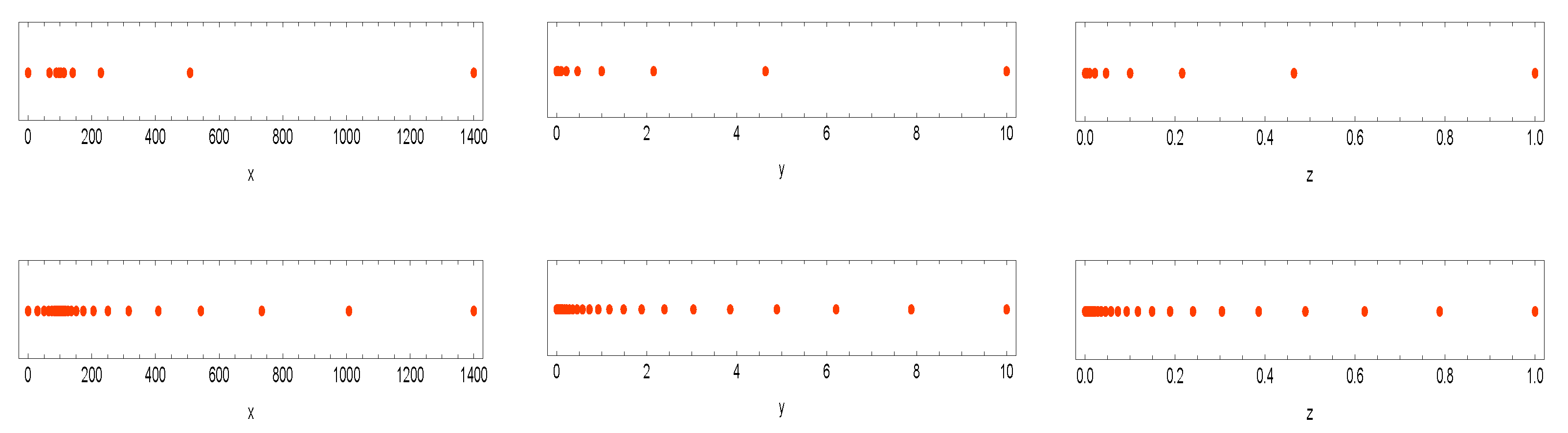
2. The Graded Meshes

For these proceedings, it is assumed that { x i } i = 1 m is a partition for x [ x min , x max ] . A well-resulted and famous non-uniform mesh can be given as follows [19,20]:
x i = Ψ ( ν i ) , 1 i m ,
where m 3 and
ν max = ν m > > ν 2 > ν 1 = ν min ,
stand for m equidistant nodes, while we have:
ν int = x right x left d 1 , ν min = sinh 1 x min x left d 1 , ν max = ν int + sinh 1 x max x right d 1 .
We, too, find that x min = 0 and x max = 14 K . The parameter υ 1 > 0 controls the nodes density on x = K . In addition, one defines
Ψ ( ν ) = x left + υ 1 sinh ( ν ) , ν min ν < 0 , x left + υ 1 ν , 0 ν ν int , x right + υ 1 sinh ( ν ν int ) , ν int < ν ν max .
Here, in (8), we consider υ 1 = K 20 , while x left = max { e 0.0025 T , 0.5 } × K , x right = K , and [ x left , x right ] [ 0 , x max ] .
The discretized nodes for the variable y, i.e., { y j } j = 1 n are constructed by:
y j = sinh ( ς j ) υ 2 , j = 1 , 2 , , n ,
wherein υ 2 > 0 furnishes a density around y = 0 . Here, we consider υ 2 = y max 500 , where y max = 10 . Additionally, ς j are the equidistant discretized nodes furnished by:
Δ ς = ( n 1 ) 1 sinh 1 y max υ 2 , ς j = ( j 1 ) Δ ς , 1 j n .
Ultimately, the non-uniform nodes for the variable z are provided as:
z k = υ 3 sinh ( ζ k ) , 1 k o ,
wherein z max = 1 and υ 3 = z max 500 is a positive value. Here, we consider that ζ k = ( Δ ζ ) ( k 1 ) , Δ ζ = 1 o 1 sinh 1 z max υ 3 . We note that the variables i , j , and k are local variables in this manuscript. It is also necessary to show such graded meshes in some plots. This is illustrated in Figure 1 for different values of m, n, and o.

3. The Weighting Coefficients for the RBF-FD Methodology

To compute the coefficients α i in the RBF-FD methodology, we take into consideration that there is a linear operator, L. Then, at y ̲ = y ̲ p , for the point locations y ̲ i , it is possible to have the following system [21]:
ϕ 1 ( y ̲ 1 ) ϕ 1 ( y ̲ 2 ) ϕ 1 ( y ̲ m ) ϕ 2 ( y ̲ 1 ) ϕ 2 ( y ̲ 2 ) ϕ 2 ( y ̲ m ) ϕ m ( y ̲ 1 ) ϕ m ( y ̲ 2 ) ϕ m ( y ̲ m ) α 1 α 2 α m = L ϕ 1 ( y ̲ ) | y ̲ = y ̲ p L ϕ 2 ( y ̲ ) | y ̲ = y ̲ p L ϕ m ( y ̲ ) | y ̲ = y ̲ p ,
wherein y ̲ denotes a d-dimensional vector quantity for a set of test functions ϕ ( y ̲ ) , 1 k m .
The generalized multiquadric RBF (GMQ RBF) is used for numerical implementations from now on, as follows ([22], Chapter 4):
ϕ ( r i ) = ( p 2 + r i 2 ) ς , 1 i m ,
wherein ς stands for an appropriate constant, the shape parameter is p, and r i = x x i stands for the Euclidean distance.
It concentrates on calculating the weighting coefficients for the GMQ RBF (for the one-dimensional case without loss of generality). To calculate the coefficients of the RBF-FD methodology, we consider three non-uniform points in a stencil and write for the first derivative [23]:
L [ ϕ ( x j ) ] i = 1 ψ α i ϕ ( x i ) , j = 1 , 2 , , ψ ,
wherein L as an operator. In fact, for ψ = 3 , we attain: { x i + θ h , x i , x i h } , θ > 0 , h > 0 , and compute (15) as follows:
f ( x i ) α i + 1 f ( x i + 1 ) + α i f ( x i ) + α i 1 f ( x i 1 ) .
In approximating the first derivative of a sufficiently differentiable function, the analytical weights corresponding to this RBF can be determined as follows [24]:
α i 1 = θ p 2 ( 9 6 ς ) h 2 ( ς 1 ) ( 4 ( ς 5 ) θ 10 ς + 29 ) 3 p 2 h ( 2 ς 3 ) ( θ + 1 ) ,
α i = ( θ 1 ) p 2 ( 6 ς 9 ) + 4 h 2 ( ς 5 ) ( ς 1 ) θ 3 p 2 h ( 2 ς 3 ) θ ,
α i + 1 = p 2 ( 6 ς 9 ) h 2 ( ς 1 ) θ ( 2 ς ( 5 θ 2 ) 29 θ + 20 ) 3 p 2 h ( 2 ς 3 ) θ ( θ + 1 ) .
In a similar way, to estimate the function’s second derivative, one has the following
f ( x i ) j = i 1 i + 1 Θ j f ( x j ) ,
and we obtain the following weighting coefficients:
Θ i 1 = 2 p 2 ( 6 ς 9 ) h 2 ( ς 1 ) 4 ( ς 5 ) θ 2 + ( 34 8 ς ) θ + 10 ς 29 3 p 2 h 2 ( 2 ς 3 ) ( θ + 1 ) ,
Θ i = 2 p 2 ( 9 6 ς ) + h 2 ( ς 1 ) 4 ( ς 5 ) θ 2 + ( 25 2 ς ) θ + 4 ( ς 5 ) 3 p 2 h 2 ( 2 ς 3 ) θ ,
Θ i + 1 = 2 p 2 ( 6 ς 9 ) h 2 ( ς 1 ) ( 2 ς ( θ ( 5 θ 4 ) + 2 ) + θ ( 34 29 θ ) 20 ) 3 p 2 h 2 ( 2 ς 3 ) θ ( θ + 1 ) .
The procedure for the discretization nodes which are on the boundaries is given along the spatial variable x, while it is similar for the other spatial variables of the PDE problem (3). The formulations (17)–(19) and (21)–(22) are fruitful from the second row to the second-to-last row, while for the first and final rows of (28) and (29), the weights are not valid on boundaries and sided estimations must be incorporated. Thus, using [25] for the stencil { x 1 , x 2 , x 3 } , we have:
f ( x 1 ) = f [ x 2 , x 1 ] f [ x 2 , x 3 ] + f [ x 3 , x 1 ] + O ( x 1 x 2 ) 2 ,
and
f ( x m ) = f [ x m 2 , x m 1 ] + f [ x m 2 , x m ] + f [ x m 1 , x m ] + O ( x m 1 x m ) 2 ,
where f [ w , q ] = ( f ( w ) f ( q ) ) ( w q ) 1 . Although we have used these approximation from the work [25], it is recalled that they are obtained by considering three unstructured points in a stencil and constructing the unique interpolating polynomial of the second degree. We then compute its first derivative in x 1 to obtain (24) or in x m to obtain (25).
In a similar manner, for the four points { { x 4 , f ( x 4 ) } , { x 3 , f ( x 3 ) } , { x 2 , f ( x 2 ) } , { x 1 , f ( x 1 ) } } , we can obtain
f ( x 1 ) = 2 ( δ x 1 , 2 + δ x 1 , 3 + δ x 1 , 4 ) δ x 1 , 2 δ x 1 , 3 δ x 1 , 4 f x 1 + 2 ( δ x 3 , 1 + δ x 4 , 1 ) δ x 1 , 2 δ x 2 , 3 δ x 2 , 4 f x 2 + 2 ( δ x 2 , 1 + δ x 4 , 1 ) δ x 1 , 3 δ x 3 , 2 δ x 3 , 4 f x 3 + 2 ( δ x 2 , 1 + δ x 3 , 1 ) δ x 1 , 4 δ x 4 , 2 δ x 4 , 3 f x 4 + O h 2 ,
where δ x ς , q = x ς x q , h is for the maximum space width along the stencil’s points. Recalling that we can also obtain:
f ( x m ) = 2 δ x m 3 , m + δ x m 2 , m + δ x m 1 , m δ x m 3 , m δ x m , m 2 δ x m , m 1 f x m + 2 δ x m 3 , m + δ x m 2 , m δ x m 3 , m 1 δ x m 1 , m 2 δ x m 1 , m f x m 1 + 2 δ x m 3 , m + δ x m 1 , m δ x m 3 , m 2 δ x m 2 , m 1 δ x m 2 , m f x m 2 + 2 δ x m 2 , m + δ x m 1 , m δ x m 2 , m 3 δ x m 1 , m 3 δ x m , m 3 f x m 3 + O h 2 .

4. Construction of Our Solver

Now, the method of lines (MOL) is employed [26,27] to semi-discretize the PDE problem. In this procedure, the spatial variables are discretized with the RBF-FD formulations we have obtained in Section 3, and we will obtain a system of ODEs. Thus, we can obtain the following differentiation matrices for the first and second derivatives of the function based on the non-uniform stencils provided in Section 2, as follows:
M x = α i , j using ( 17 ) i j = 1 , α i , j using ( 18 ) i j = 0 , α i , j using ( 19 ) j i = 1 , 0 otherwise ,
and
M x x = Θ i , j using ( 21 ) i j = 1 , Θ i , j using ( 22 ) i j = 0 , Θ i , j using ( 23 ) j i = 1 , 0 otherwise .
We come up with the matrices (28) and (29) form the weights in Section 3. To be more precise, we must consider a loop on the set of discretization points. Then, each time, a stencil with three non-uniform points is considered and the corresponding weights are computed. These weights are written in the corresponding rows of the differentiation matrix. For instance, if we take the second node of the set of discretization points, then the three-point stencil consists of the first, second the third nodes. After we have obtained the weights, they will be written in the second row (corresponding to the second node of the discretization points) of the differentiation matrix.
Now, we denote the Kronecker product by ⊗ and consider I = I x I y I z , as an N × N identity matrix where N = o × n × m , I x is the m × m unit matrix for x, and a similar operation is conducted for I y and I z . The PDE (3) has several diffusions, reactions and advection terms. Let us consider the first term of this PDE as follows:
1 2 x 2 y 2 U ( x , y , z , t ) x 2 ,
which can be semi-discretized along space using matrix notations, as follows:
1 2 X 2 Y ( M x x I y I z ) ,
where the square matrices M x , and M x x are derived via the corresponding weights (28) and (29), respectively. Furthermore, X is a diagonal and sparse matrix, as follows:
X = diag x 1 , x 2 , , x m I y I z .
Hence, the MOL procedure on (3) leads to the following matrix:
B = 1 2 X 2 Y ( M x x I y I z ) + 1 2 σ 1 2 Y ( I x M y y I z ) + 1 2 σ 2 2 Z ( I x I y M z z ) + ρ 12 σ 1 X Y ( M x M y I z ) + ρ 13 σ 2 X ( Y Z ) 1 2 ( M x I y M z ) + ρ 23 σ 1 σ 2 ( Y Z ) 1 2 ( I x M y M z ) + Z X ( M x I y I z ) + κ ( η I Y ) ( I x M y I z ) + a ( β 0 I Z ) ( I x I y M z ) z I .
In addition, the square matrices M y , M z , M y y , and M z z , are similarly derived via the corresponding weights. Furthermore, Z , and Y are diagonal and sparse matrices, as follows:
Z = I x I y diag z 1 , z 2 , , z o ,
Y = I x diag y 1 , y 2 , , y n I z ,
The derivation of (33) is based on the differentiation matrices and the structure of the 3D PDE (3). The function b ( T t ) can be defined by:
b ( τ ) = c 1 c 2 exp ( c 3 τ ) β 0 ,
where c 1 , c 2 , and c 3 are fixed parameters, and τ = T t . The advantage of the approximation in (36) when c 2 and c 3 are not zero is that, with such an approximation, we can get rid of the time-dependent function b, and thus the system matrix B is constant.
Now, finally, we determine that:
u ( t ) = B u ( t ) .
The boundaries for the spaces x , y and z are defined by [12]:
U ( x , y , z , t ) = x ,   y = y max ,
U x ( x , y , z , t ) = 1 , x = x max ,
U ( x , y , z , t ) = 0 , x = 0 ,
U z ( x , y , z , t ) = 0 , z = z max .
Once y = 0 and z = 0 , the problem (3) is degenerate, and boundary conditions should not be incorporated.
By imposing such boundaries, finally, a set of ODEs is deduced by:
u ( t ) = B ¯ u ( t ) = F ( t , u ( t ) ) ,
wherein B ¯ is the coefficient matrix including all the conditions of the boundary. The boundary conditions (38)–(41) of the PDE are non-homogeneous. However, the system ODE (42) which comes from the semi-discretization is homogeneous. This is because the boundaries are imposed by differentiating over time, so for the Neumann conditions, we write the second-order estimation along each boundary and then they are differentiated over time. The coefficients will then be replaced as new rows to the matrix B in order to obtain B ¯ .

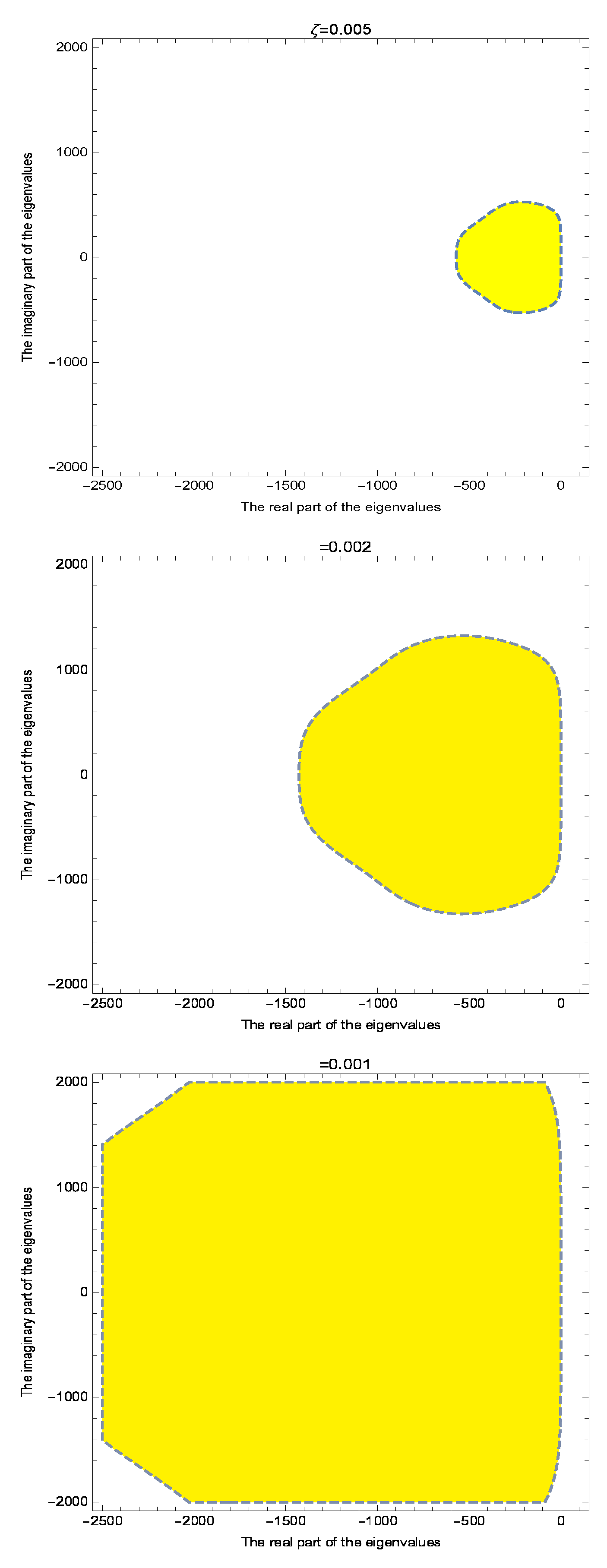
5. The Time-Stepping Solver

The solution in the closed-form for the system of stiff ODEs (42) can be given by:
u ( t ) = e t B ˜ u ( 0 ) ,
wherein u ( 0 ) is initial condition (payoff) based on the type of the option. Finding the final approximated solution based on (43) needs the calculation of matrix exponential as a matrix function, which is a time-consuming procedure in a general setting.
Now, consider that u ι as an approximate to u ( t ι ) . We construct the explicit time-integrating scheme as follows. Consider k + 1 equidistant points along time, a temporal step size ζ = T k > 0 , t ι + 1 = ζ + t ι , u 0 = u ( 0 ) and 0 ι k , then the Runge–Kutta (RK) method with s stages [28] can be written as follows:
g i = u ι + ζ j = 1 s k j a i , j , k i = F ζ c i + t ι , g i , u ι + 1 = u ι + ζ i = 1 s q i k i ,
wherein F ( · , · ) = B ˜ u ( t ) . Note that basically, we consider:
c i = j = 1 s a i , j , 1 i s .
Explicit RK solvers are a specific case when
Λ = [ a i , j ] ,
to be lower in a strictly triangular sense. Hence, we can attain a solver with sixth-order convergence by considering [29]:
Λ = 0 0 0 0 0 0 0 1 0 0 0 0 0 0 3 8 1 8 0 0 0 0 0 8 27 2 27 8 27 0 0 0 0 3 3 p 1 7 392 p 1 7 49 6 p 1 7 49 3 p 1 21 392 0 0 0 3 17 p 1 + 77 392 p 1 7 49 8 p 1 49 3 121 p 1 + 21 1960 p 1 + 6 5 0 0 7 p 1 + 22 12 2 3 2 7 p 1 5 9 7 3 p 1 2 20 7 9 p 1 + 49 90 7 p 1 7 18 0 ,
with p 1 = 21 1 / 2 , C = ( 1 , 1 / 2 , 2 / 3 , ( 7 p 1 ) / 14 , ( 7 + p 1 ) / 14 , 1 ) , and q = ( 9 / 180 , 0 , 64 / 180 , 0 , 49 / 180 , 49 / 180 , 9 / 180 ) .
Here, the choice c 1 = 0 in (45) led to an explicit solver having sixth order of convergence along time with seven stages. This means that the total accumulated error is O ( ζ 6 ) and the local truncation error is O ( ζ 7 ) , ([30], Chapter 8). It is remarked that (44) is just an application of literature in the process of resolving (3), which is considered the main result in this work.
Such a higher-order scheme is employed over time to solve (42), since the spatial order is four and there is a non-smoothness at the strike price for the payoff function. This automatically affects the accuracy of the numerical solution when marching along time. Hence, an explicit easy-to-implement solver of higher convergence rate help derive an effective numerical method.
Theorem 1.
Consider that (42) reads the well-known Lipschitz condition. Hence, one has a conditional temporal-stable iterative method according to (44)–(46) for solving (42).
Proof. 
The existence and uniqueness can be obtained by the assumption of satisfying in the Lipschitz condition. Thus, by incorporating the solver (44)–(46) on the set of ODEs, (42) provides the relation below [31]:
u ι + 1 = I + ζ B ˜ + ( ζ B ˜ ) 2 2 ! + ( ζ B ˜ ) 3 3 ! + ( ζ B ˜ ) 4 4 ! + ( ζ B ˜ ) 5 5 ! + ( ζ B ˜ ) 6 6 ! ( ζ B ˜ ) 7 2160 u ι .
Hence, the A-stability is
1 + ζ λ i + ( ζ λ i ) 2 2 + ( ζ λ i ) 3 6 + ( ζ λ i ) 4 24 + ( ζ λ i ) 5 120 + ( ζ λ i ) 6 720 ( ζ λ i ) 7 2160 1 ,
which is due to (47) for any λ i as the eigenvalue of B ˜ . The condition of stability can be now expressed as follows:
1 + ζ λ max + ( ζ λ max ) 2 2 + ( ζ λ max ) 3 6 + ( ζ λ max ) 4 24 + ( ζ λ max ) 5 120 + ( ζ λ max ) 6 720 ( ζ λ max ) 7 2160 1 .
Considering Γ = ζ λ max , the inequality (49) furnishes a non-linear scalar equation, as follows:
Γ 7 3 Γ 6 18 Γ 5 90 Γ 4 360 Γ 3 1080 Γ 2 2160 Γ 4320 = 0 ,
with { 2.61051 1.23959 i , 2.61051 + 1.23959 i , 0.720604 2.58827 i , 0.720604   + 2.58827 i , 0.900758 2.88184 i , 0.900758 + 2.88184 i , 7.86071 } as its roots. Equivalently, one could calculate the following condition on ζ using (44)–(46) when solving (42):
ζ 7.86 Real λ max .
This inequality on the eigenvalues of B ˜ will determine the conditional temporal stability bounds of the presented method when solving (3). Thus, it completes the proof. □
Now, an inquiry might arise. The inequality (51) depends on the real part of the largest eigenvalues of matrix B ˜ . On the other hand, on the proposed graded mesh, the largest eigenvalue of B ˜ is usually large, so the choice of the time-step ζ could be restrictive. Thus, it seems the proposed numerical method is not quite stable! In fact, the real part of the largest eigenvalue of B ˜ might be larger due to employing the graded mesh, but because of this, we need to employ a higher-order explicit method which has large numerical stability region. To illustrate this further, in Figure 2, we have drawn the numerical stability region for different time step sizes. It is clear that when ζ is changed at a smaller size, it has a very big impact on the numerical stability region, and this upholds our choice for the time stepping solver. It is also pointed out that the application of the graded mesh leads to a lower number of discretization points to obtain the required accuracy, and this means that the resulting B ˜ is basically of lower dimension when we want to obtain the same accuracy on uniform meshes.

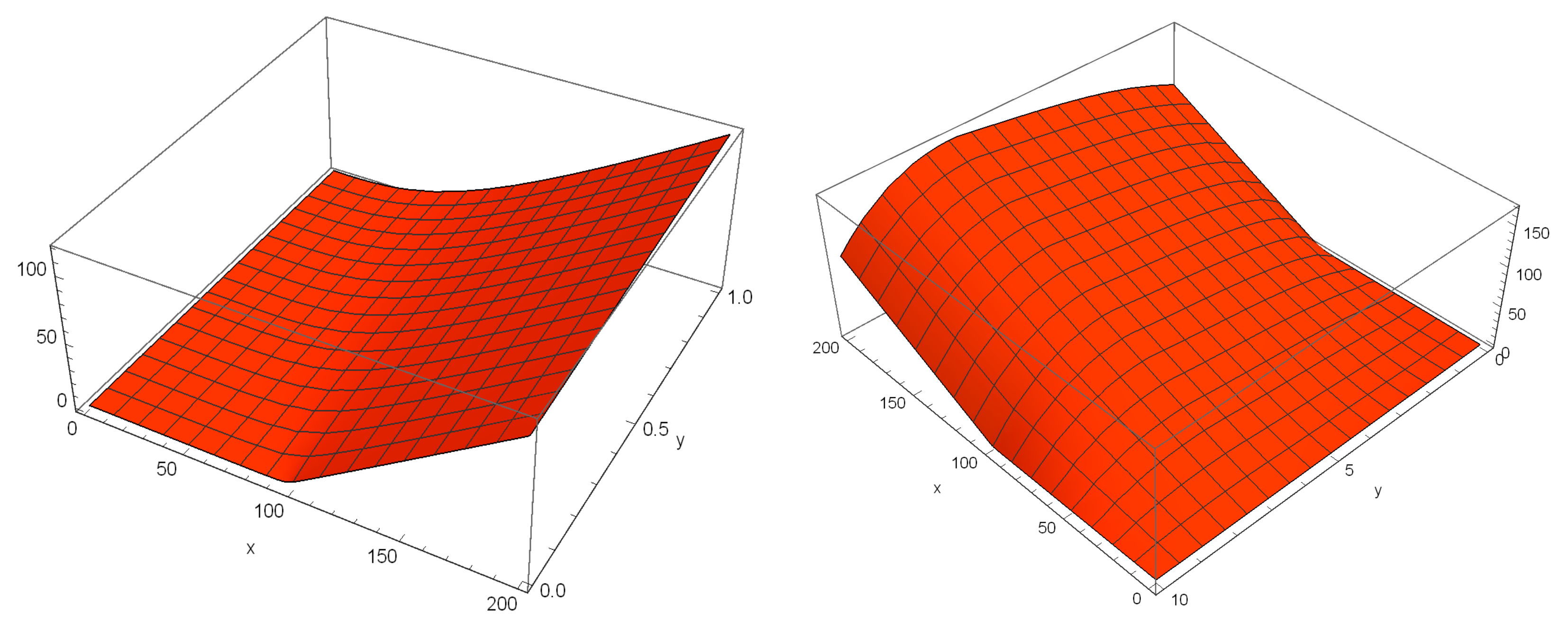
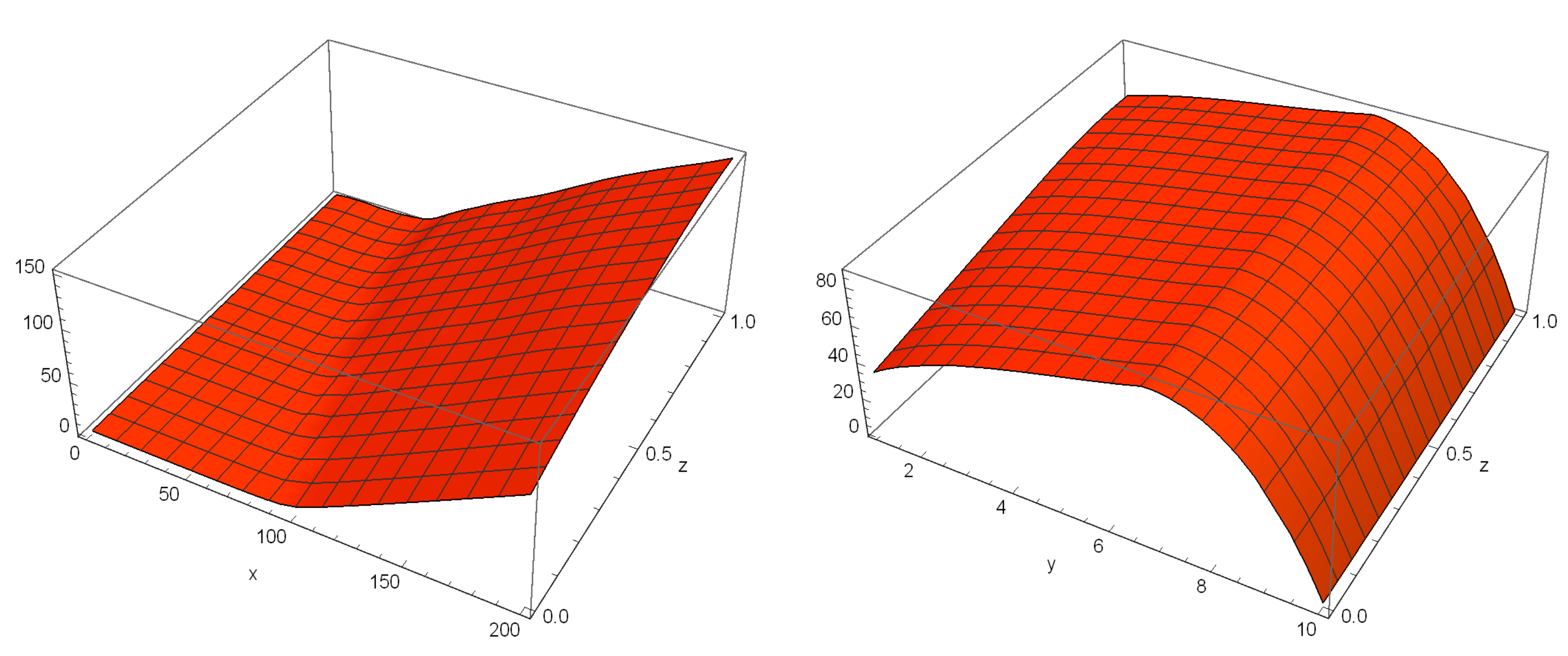
6. Financial Experiments

The goal here is to calculate the efficiency of different methods to numerically resolve (3) on a same computational domain when K = 100 $ , T = 1 year, y 0 = 0.04 , z 0 = 10 % . The outcome of tests must be compared with the associated outcome of existing solvers to arrive at a logical and valid conclusion. The following solvers are used:
  • The quadratically convergent FD method on uniform meshes and the first-order explicit Euler’s scheme denoted by FDS.
  • The scheme with non-equally spaced node distribution (via the Douglas time-stepping method) given in [19], (shown by THM).
  • The method presented by Soleymani et al. in [25] and shown by SAM.
  • The presented method of Section 2, Section 3, Section 4 and Section 5 shown by RBF-FD-PM.
We used Mathematica 12.0 [32] for programming, with double-precision arithmetic. The absolute error is given by:
ε = u ref u num u ref ,
wherein u ref and u num are the referenced and numerical solutions, respectively. u ref was obtained from the literature.
One effective procedure with which to calculate the parameter of the shape is p = 5 max { Δ x i } , where 1 i m 1 , and Δ x i are the increments along the variable mesh.
Three different types of parameters have been considered in Table 1. Table 2, Table 3 and Table 4 show the convergence history of different solvers in Cases I-III, while also revealing that RBF-FD-PM is better than the FDS and the THM methods.
The reference solutions for the Cases I-II-III are 13.444, 6.839 and 3.890, respectively [25]. A numerical solution is presented for Case II in Figure 3, showing the stability of the numerical solution using RBF-FD-PM.
It can be inferred from the findings of performance outcomes, displayed in Table 2, Table 3 and Table 4, that the presented solver is numerically more effective compared to the available methods. Similar computational tests, conducted on different parameter settings, largely uphold the above conclusions.
We note that implicit schemes might be attractive for solving the system of ODEs (42), since they mostly do not rely on the selection of the step size. However, this topics needs further investigation, since the problem with implicit solvers is that a large set of non-linear algebraic equations must be solved via a Newton-type method, which increases the computational elapsed time.

7. Conclusions

To computationally and efficiently solve the PDE problem (3), this work began by considering the RBF-FD formulations corresponding to the GMQ RBF in Section 3 based on the graded meshes discussed in Section 2. Then, the MOL for (3) was performed using sparse arrays in order to maintain and develop the sparsity as the dimension of the problem grew. Then in Section 4, a sixth-order explicit solver from the RK family of methods was introduced. It was shown that the contributed scheme is fast and stable, with error bounds O ( ζ 6 ) . The numerical results given in Section 6 overwhelmingly upheld the theoretical discussions of the paper. Hence, the proposed solver can be used to solve the important 3D time-dependent PDE (3) in practice.

Author Contributions

Conceptualization, X.M.; formal analysis, X.M. and S.S.; funding acquisition, M.Z.U.; investigation, X.M., M.Z.U. and S.S.; methodology, X.M. and S.S.; supervision, M.Z.U.; validation, X.M., M.Z.U. and S.S.; writing—original draft, X.M. and S.S.; writing—review and editing, X.M., M.Z.U. and S.S. All authors have read and agreed to the published version of the manuscript.

Funding

This research received no external funding.

Institutional Review Board Statement

Not applicable.

Informed Consent Statement

Not applicable.

Data Availability Statement

For the data availability statement, we state that data sharing is not applicable to this article, as no new data were created in this study.

Acknowledgments

This research work was funded by Institutional Fund Projects under grant no. (IFPIP: 1417-130-1443). The authors gratefully acknowledge technical and financial support provided by the Ministry of Education and King Abdulaziz University, DSR, Jeddah, Saudi Arabia.

Conflicts of Interest

The authors declare that they have no known competing financial interest or personal relationship that could have appeared to influence the work reported in this paper.

References

  1. Adhikari, R. Foundations of Computational Finance. Math. J. 2020, 22, 1–59. [Google Scholar] [CrossRef]
  2. Itkin, A. Pricing Derivatives Under Lévy Models: Modern Finite-Difference and Pseudo–Differential Operators Approach; Birkhäuser: Basel, Switzerland, 2017. [Google Scholar]
  3. Guo, S.; Grzelak, L.; Oosterlee, C.W. Analysis of an affine version of the Heston-Hull-White option pricing partial differential equation. Appl. Numer. Math. 2013, 72, 143–159. [Google Scholar] [CrossRef] [Green Version]
  4. Heston, S.L. A closed-form solution for options with stochastic volatility with applications to bond and currency options. Rev. Finan. Stud. 1993, 6, 327–343. [Google Scholar] [CrossRef] [Green Version]
  5. Cao, J.; Lian, G.; Roslan, T.R.N. Pricing variance swaps under stochastic volatility and stochastic interest rate. Appl. Math. Comput. 2016, 277, 72–81. [Google Scholar] [CrossRef]
  6. Hull, J.; White, A. Using Hull-White interest rate trees. J. Deriv. 1996, 4, 26–36. [Google Scholar] [CrossRef]
  7. Ampun, S.; Sawangtong, P.; Sawangtong, W. An analysis of the fractional-order option pricing problem for two assets by the generalized Laplace variational iteration approach. Fractal Fract. 2022, 6, 667. [Google Scholar] [CrossRef]
  8. Zhang, X.; Yang, J.; Zhao, Y. Numerical solution of time fractional Black-Scholes model based on Legendre wavelet neural network with extreme learning machine. Fractal Fract. 2022, 6, 401. [Google Scholar] [CrossRef]
  9. Cox, J.C.; Ingersoll, J.E.; Ross, S.A. A theory of the term structure of interest rates. Econometrica 1985, 53, 385–407. [Google Scholar] [CrossRef]
  10. Grzelak, L.A.; Oosterlee, C.W. On the Heston model with stochastic interest rates. SIAM J. Finan. Math. 2011, 2, 255–286. [Google Scholar] [CrossRef] [Green Version]
  11. Djeutcha, E.; Fono, L.A. Pricing for options in a Hull-White-Vasicek volatility and interest rate model. Appl. Math. Sci. 2021, 15, 377–384. [Google Scholar] [CrossRef]
  12. Haentjens, T. Efficient and stable numerical solution of the Heston-Cox-Ingersoll–Ross partial differential equation by alternating direction implicit finite difference schemes. Int. J. Comput. Math. 2013, 90, 2409–2430. [Google Scholar] [CrossRef]
  13. Fornberg, B. A Practical Guide to Pseudospectral Methods; Cambridge University Press: Cambridge, UK, 1996. [Google Scholar]
  14. Kadalbajoo, M.K.; Kumar, A.; Tripathi, L.P. Radial-basis-function–based finite difference operator splitting method for pricing American options. Int. J. Comput. Math. 2018, 95, 2343–2359. [Google Scholar] [CrossRef]
  15. Vanani, S.K.; Hafshejani, J.S.; Soleymani, F.; Khan, M. Radial basis collocation method for the solution of differential-difference equations. World Appl. Sci. J. 2011, 13, 2526–2530. [Google Scholar]
  16. Farahmand, G.; Lotfi, T.; Ullah, M.Z.; Shateyi, S. Finding an efficient computational solution for the Bates partial integro-differential equation utilizing the RBF-FD scheme. Mathematics 2023, 11, 1123. [Google Scholar] [CrossRef]
  17. Liu, T.; Ullah, M.Z.; Shateyi, S.; Liu, C.; Yang, Y. An efficient localized RBF-FD method to simulate the Heston-Hull-White PDE in finance. Mathematics 2023, 11, 833. [Google Scholar] [CrossRef]
  18. Milovanović, S.; von Sydow, L. A high order method for pricing of financial derivatives using radial basis function generated finite differences. Math. Comput. Simul. 2020, 174, 205–217. [Google Scholar] [CrossRef] [Green Version]
  19. Haentjens, T.; In’t Hout, K.J. Alternating direction implicit finite difference schemes for the Heston-Hull-White partial differential equation. J. Comput. Financ. 2012, 16, 83–110. [Google Scholar] [CrossRef]
  20. Kluge, T. Pricing Derivatives in Stochastic Volatility Models Using the Finite Difference Method. Ph.D. Thesis, Technische Universität Chemnitz, Chemnitz, Germany, 2002. [Google Scholar]
  21. Milovanović, S.; von Sydow, L. Radial basis function generated finite differences for option pricing problems. Comput. Math. Appl. 2018, 75, 1462–1481. [Google Scholar]
  22. Fasshauer, G.E. Meshfree Approximation Methods with MATLAB; World Scientific Publishing: Singapore, 2007. [Google Scholar]
  23. Wright, G.B.; Fornberg, B. Scattered node compact finite difference-type formulas generated from radial basis functions. J. Comput. Phys. 2006, 212, 99–123. [Google Scholar] [CrossRef]
  24. Soleymani, F.; Zhu, S. RBF-FD solution for a financial partial-integro differential equation utilizing the generalized multiquadric function. Comput. Math. Appl. 2021, 82, 161–178. [Google Scholar] [CrossRef]
  25. Soleymani, F.; Akgül, A.; Karatas Akgül, E. On an improved computational solution for the 3D HCIR PDE in finance. Analele Stiintifice Ale Univ. Ovidius Constanta Ser. Mat. 2019, 27, 207–230. [Google Scholar] [CrossRef] [Green Version]
  26. Knapp, R. A method of lines framework in Mathematica. J. Numer. Anal. Indust. Appl. Math. 2008, 3, 43–59. [Google Scholar]
  27. Meyer, G.H. The Time-Discrete Method of Lines for Options and Bonds, A PDE Approach; World Scientific Publishing: Singapore, 2015. [Google Scholar]
  28. Sofroniou, M.; Knapp, R. Advanced Numerical Differential Equation Solving in Mathematica; Wolfram Mathematica, Tutorial Collection; Wolfram: Champaign, IL, USA, 2008. [Google Scholar]
  29. Luther, H.A. An explicit sixth-order Runge-Kutta formula. Math Comput. 1967, 22, 434–436. [Google Scholar] [CrossRef]
  30. Keskin, A.Ü. Ordinary Differential Equations for Engineers; Springer International Publishing: Cham, Switzerland, 2019. [Google Scholar]
  31. Shampine, L.F. Numerical Solution of Ordinary Differential Equations; Chapman and Hall: London, UK, 1994. [Google Scholar]
  32. Wellin, P.R.; Gaylord, R.J.; Kamin, S.N. An Introduction to Programming with Mathematica; Cambridge University Press: Cambridge, UK, 2005. [Google Scholar]
Figure 1. Distributions of the nodes along each spatial variables, for m = n = o = 10 at the top and m = m = o = 30 at the bottom.
Fractalfract 07 00316 g001
Figure 2. The numerical stability region of (44)–(46) for different values of ζ , i.e., ζ = 0.005 , ζ = 0.002 and ζ = 0.001 .
Fractalfract 07 00316 g002
Figure 3. Numerical solution of the HCIR PDE in Case II. Top-left: for u ( x , y , 0.024 , 1 ) on 0 x 200 , 0 y 1 , Top-right: for u ( x , y , 0.024 , 1 ) on 0 x 200 , 0 y 10 , Bottom-left: for u ( x , 0.04 , z , 1 ) on 0 x 200 , 0 z 1 and Bottom-right: for u ( 100 , y , z , 1 ) on 1 y 10 , 0 z 1 .
Fractalfract 07 00316 g003aFractalfract 07 00316 g003b
Table 1. The values of the constants in PDE (3).
Case ICase IICase III
c 3 002.10
c 2 000.014
c 1 0.050.0550.034
a0.200.160.22
σ 2 0.030.030.11
σ 1 0.040.901.00
η 0.120.040.09
ρ 23 0.40.1−0.2
ρ 13 0.20.2−0.5
ρ 12 0.6−0.5−0.3
κ 3.00.31.0
K100100100
T110.25
Table 2. Computational results for Case I.
MethodmnoN ζ u ε Time
FDS
10101010000.00121.187 5.75 × 10 1 0.49
16121223040.00055.887 5.62 × 10 1 1.07
30161676800.00017.542 4.38 × 10 1 11.23
40202016,0000.0000510.698 2.04 × 10 1 52.96
54222226,1360.0000210.738 2.01 × 10 1 382.17
THM
10101010000.00112.216 9.12 × 10 2 0.68
16121223040.000513.046 2.95 × 10 2 1.81
30161676800.000113.325 8.82 × 10 3 15.31
40202016,0000.0000513.376 4.99 × 10 3 99.67
54222226,1360.0000213.404 2.92 × 10 3 473.52
SAM
10101010000.00114.944 1.11 × 10 1 0.63
16121223040.000513.804 2.68 × 10 2 1.68
30161676800.000113.515 5.28 × 10 3 21.54
40202016,0000.0000513.477 2.49 × 10 3 107.49
54222226,1360.0000213.457 9.87 × 10 4 499.67
RBF-FD-PM
10101010000.00214.846 1.04 × 10 1 0.62
16121223040.00113.762 2.36 × 10 2 1.62
30161676800.000413.499 4.09 × 10 3 20.81
40202016,0000.000113.471 2.00 × 10 3 101.19
54222226,1360.0000413.455 8.18 × 10 4 477.28
Table 3. Computational results and comparisons for the Case II.
MethodmnoN ζ u ε Time
FDS
8885120.00247.829 5.99 × 10 0 0.27
14101014000.00055.469 2.00 × 10 1 0.71
20141233600.0002514.786 1.16 × 10 1 2.13
24161453760.000112.960 8.95 × 10 1 6.91
32181810,3680.000058.599 2.57 × 10 1 28.64
45242019,8000.0000256.456 5.59 × 10 2 178.43
THM
8885120.0025.010 2.67 × 10 1 0.30
14101014000.00056.440 5.83 × 10 2 0.69
20141233600.000256.672 2.43 × 10 2 1.97
24161453760.00016.729 1.59 × 10 2 6.58
32181810,3680.000056.797 6.02 × 10 3 32.44
45242019,8000.0000256.830 1.28 × 10 3 180.59
SAM
8885120.0025.794 1.52 × 10 1 0.35
14101014000.00056.628 3.07 × 10 2 0.96
20141233600.000256.759 1.16 × 10 2 3.11
24161453760.00016.776 9.07 × 10 3 13.37
32181810,3680.000056.809 4.30 × 10 3 57.16
45242019,8000.0000256.833 8.52 × 10 4 232.76
RBF-FD-PM
8885120.0045.861 1.43 × 10 1 0.33
14101014000.0016.501 4.94 × 10 2 0.90
20141233600.00046.760 1.15 × 10 2 3.03
24161453760.00026.786 7.74 × 10 3 12.69
32181810,3680.00016.826 1.90 × 10 3 55.84
45242019,8000.000046.834 7.31 × 10 4 224.21
Table 4. Computational results and comparisons for Case III.
MethodmnoN ζ u ε Time
FDS
8885120.0020.857 7.79 × 10 1 0.10
14101014000.00052.124 4.53 × 10 1 0.27
20141233600.000252.976 2.34 × 10 1 1.08
24161453760.00013.214 1.73 × 10 1 3.54
THM
8885120.0023.210 1.74 × 10 1 0.30
14101014000.00053.528 9.30 × 10 2 1.01
20141233600.000253.604 7.35 × 10 2 1.51
24161453760.00013.694 5.03 × 10 2 4.92
SAM
8885120.0023.329 1.44 × 10 1 0.26
14101014000.00053.539 9.02 × 10 2 0.87
20141233600.000253.719 4.39 × 10 2 1.48
24161453760.00013.924 8.74 × 10 3 4.76
RBF-FD-PM
8885120.00253.413 1.22 × 10 1 0.23
14101014000.0006253.610 7.19 × 10 2 0.78
20141233600.00043.816 1.90 × 10 2 1.39
24161453760.000253.918 7.19 × 10 3 4.67
Disclaimer/Publisher’s Note: The statements, opinions and data contained in all publications are solely those of the individual author(s) and contributor(s) and not of MDPI and/or the editor(s). MDPI and/or the editor(s) disclaim responsibility for any injury to people or property resulting from any ideas, methods, instructions or products referred to in the content.

