Adaptive Neural Network Synchronization Control for Uncertain Fractional-Order Time-Delay Chaotic Systems

Abstract

We propose an adaptive radial basis (RBF) neural network controller based on Lyapunov stability theory for uncertain fractional-order time-delay chaotic systems (FOTDCSs) with different time delays. The controller does not depend on the system model and can achieve synchronous control under the condition that nonlinear uncertainties and external disturbances are completely unknown. Stability analysis showed that the error system asymptotically tended to zero in combination with the relevant lemma. Numerical simulation results show the effectiveness of the controller.

1. Introduction

The theory of fractional calculus has been developed for more than 300 years, but due to a lack of effective computing means, its research has been in the field of pure mathematics, and its development has been slow. With the continuous development of computer technology, the application of fractional calculus in engineering practice and physics has become a hotspot [1,2,3,4]. Compared with integer-order differential equations, fractional-order calculus equations can describe natural phenomena more accurately [5,6]. Therefore, they are universal to studying fractional-order systems.

Chaos is a special movement state of a nonlinear system that is the unity of order and disorder; it is easily affected by external conditions and especially sensitive to the initial value of the system. With the gradual deepening of people’s understanding of chaotic systems, scholars have found that fractional-order chaotic systems have almost all the characteristics of integer-order chaotic systems. Because of their historical memory characteristics, fractional-order chaotic systems often have more complex dynamic behaviors than those of integer-order chaotic systems. Time delay is a common phenomenon in nature [7]. Due to the influence of friction, machinery, and other practical factors, there are always time delays in practical systems, such as physics, machinery, economy, biology, and engineering. In addition, time delay has an important impact on the dynamic characteristics of the system. When the change in the system on both the current and past states, the system is called a time-delay system. The existence of a time delay renders the fractional chaotic system more complex, and has broad application prospects in image encryption [8], secure communication [9], and biomedicine [10].

Chaos synchronization control means that the state trajectory of the response system can completely follow the drive system under the action of the controller. In 1990, chaos synchronization was first proposed by Pecora and Carroll, who successfully realized the synchronization of two systems with the same structure under different initial conditions [11]. As a typical feature of nonlinear systems, the synchronization of chaotic systems has been studied extensively, and a large number of synchronization control methods were proposed [12,13,14,15,16,17]. In [18], a linear controller was designed for the synchronization control of fractional-order financial chaotic systems with time delay in the absence of uncertainties and external disturbances. This controller realized the active synchronization control of fractional-order Financial chaotic systems with time delay. Liu et al. [19] investigated a sliding-mode controller that had been designed for the synchronization control of FOTDCSs with uncertainties. The controller realized the self-synchronization of FOTDCSs, but required that uncertainties be bounded and did not consider external disturbances. In addition, the controller could not achieve synchronization with different structures. In [20,21], the authors adopted active control to directly eliminate the nonlinear term, rendering the coefficient matrix of the system constant and realizing the hybrid projection synchronization of FOTDCSs. However, its control cost was large, and when there were unknown uncertainties in the system, this method could not achieve the expected control effect. Li et al. [22] realized the impulse synchronization of FOTDCSs, but the controller needed to know the coefficient matrix of the linear part of the drive and the response system, which was highly dependent on the system model. When there are uncertainties or external disturbances in the system, it is difficult for this method to achieve synchronization control. Velmurugan et al. [23] proposed hybrid projection synchronization on the basis of the neural network fractional time-delay memristor model, which also uses active control to eliminate nonlinear terms. Second, it did not consider the aging and decay of memristor elements (that is, there were unknown uncertainties in the system). Luo et al. [24] investigated the fractional-order MEMS model and achieved the active synchronization of the model through a Chebyshev neural network. However, this idea was only aimed at special models and is not universal. In addition, all the above control methods are only applicable to synchronous control when the time delays of the drive and response systems are the same.

In an actual physical system, the system may be affected by external disturbances, and the aging and attenuation of components exist in the running process of the system. The above factors hinder the ideal model from accurately describing the actual physical system. On the basis of the above considerations, this paper mainly focuses on the synchronization control of uncertain FOTDCSs based on adaptive RBF neural networks. On the one hand, an RBF neural network, as a local approximation network, could approximate any continuous function with arbitrary precision. So, an RBF neural network can be used to estimate an unknown system type. On the other hand, adaptive control can eliminate the influence of uncertainty and complex factors by automatically adjusting the relevant parameters of the controller, so that the controller could adapt to the controlled object and the environment. Under the action of the designed synchronous controller, the synchronization error asymptotically approaches zero. The novelty and contributions of this paper are as follows:

(1)

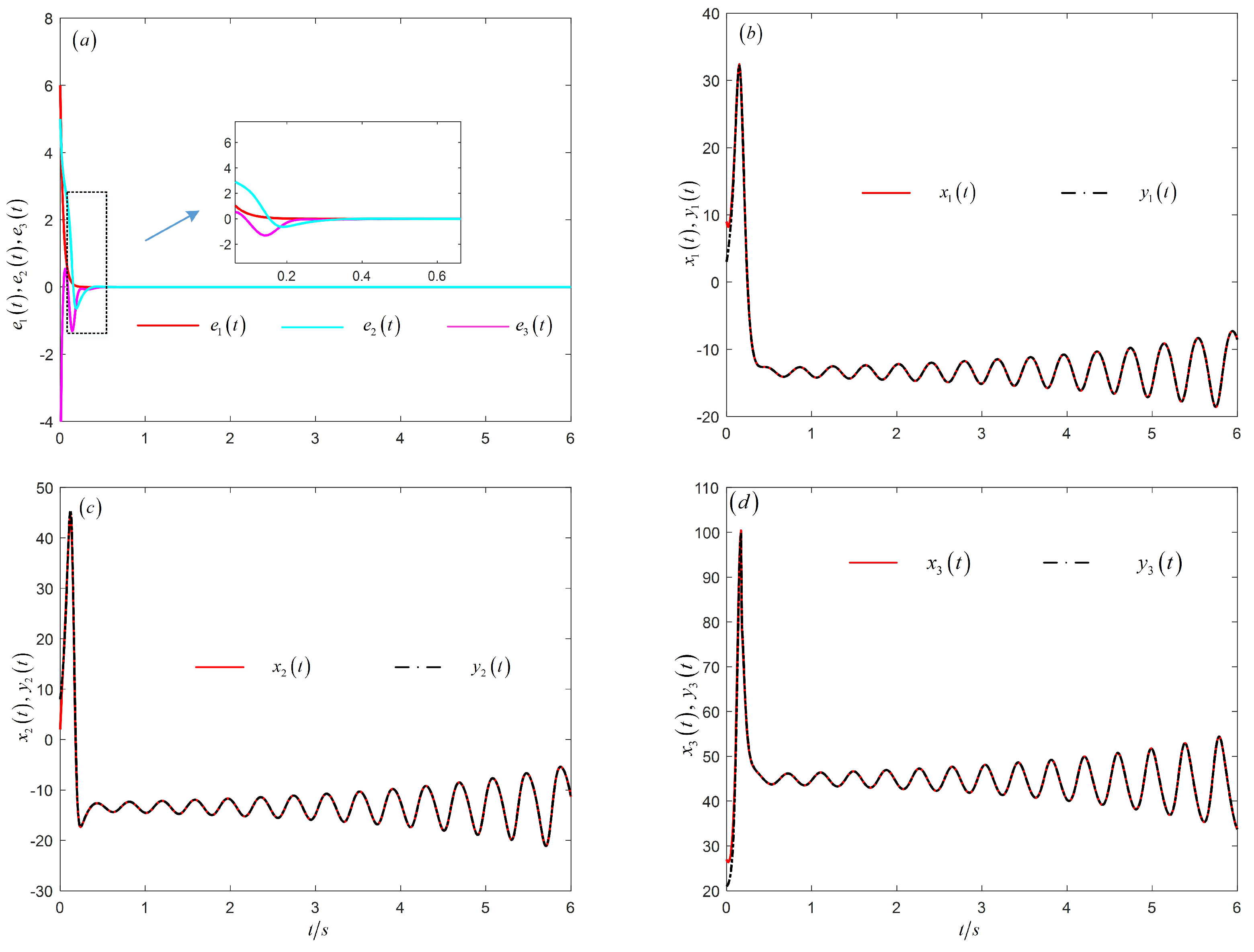
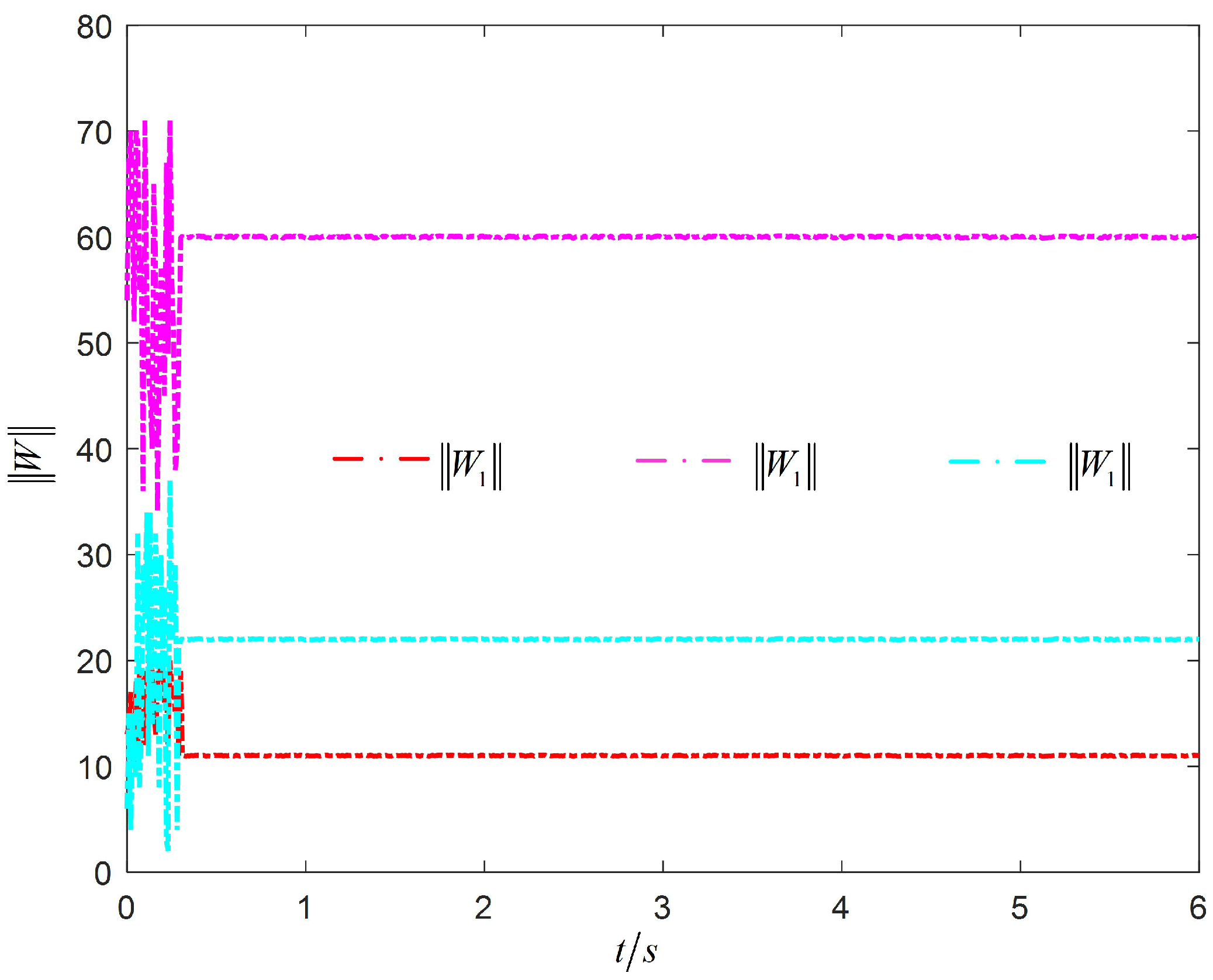
On the basis of Barbarat’s lemma, an adaptive RBF neural network controller was designed that realizes the synchronization control of FOTDCSs with nonlinear uncertainty and external disturbance.

(2)

When the driving system and the response system have different time delays, they could also achieve synchronization under the action of the controller.

(3)

A numerical simulation realized the synchronous control of the uncertain fractional time-delay Liu chaotic system and the uncertain fractional time-delay financial chaotic system. The theoretical proof and simulation results show the effectiveness of the controller.

The rest of this paper is arranged as follows: In Section 2, the preliminaries and radial basis neural network models are given. In Section 3, the synchronization controller and stability analysis based on a radial basis function neural network are presented. In Section 4, a numerical simulation is provided. Lastly, some conclusions are drawn in Section 5.

2. Preliminaries

2.1. Introduction to Fractional Calculus

There are three different definitions of fractional calculus: the Caputo derivative [25], Riemann–Liouville (R–L) derivative [26], and Grünwald–Letnikov (G–L) derivative [27]. This paper is based on Caputo’s definition; the Caputo derivative is defined as follows:

$$D_t^{\alpha }f\left(t\right)=\frac{1}{\Gamma (n-\alpha )}{\int }_0^t\frac{f^{\left(n\right)}\left(\tau \right)}{{(t-\tau )}^{(\alpha -n+1)}}d\tau ,$$

(1)

The fractional Caputo integral is defined as follows:

$$D_t^{-\alpha }f\left(t\right)=\frac{1}{\Gamma \left(\alpha \right)}{\int }_0^t{(t-\alpha )}^{(\alpha -1)}f\left(\tau \right)d\tau ,$$

(2)

where fractional order $\alpha >0$, and n is a smaller integer that is greater than $\alpha$, namely, $n-1<\alpha <n$. $\Gamma (·)$ is the Gamma function, defined as $\Gamma \left(\alpha \right)={\int }_0^t{t}^{(\alpha -1)}{e}^{-t}dt$. In addition, the fractional Caputo differential is Laplace-transformed as follows:

$$\mathcal{L}\left\{D_t^{\alpha }f\left(t\right),s\right\}=s^{\alpha }F\left(s\right)-\sum _{k=0}^{n-1}{s}^{\alpha -k-1}{f}^{\left(k\right)}\left(0\right),$$

(3)

where $F\left(s\right)$ is the Laplace transform of $f\left(t\right)$, and $h^{\left(k\right)}\left(0\right)$ are the initial conditions. Since the subsequent stability proof of the system needs to use the properties of fractional calculus, several properties are given in the following.

Proposition 1 

([28]). If $x\left(t\right)\in C^1[0,T](T>0)$, then $D_t^{\alpha }{D}_t^{\alpha -1}x\left(t\right)=x\left(t\right)$.

Proposition 2

([29]). If $x\left(t\right)\in R$, then there is $D_t^{\alpha -1}\left|x\left(t\right)\right|\ge 0$ and $D_t^{\alpha -1}\left|x\left(t\right)\right|\ge D_t^{\alpha -1}x\left(t\right)$.

Proposition 3 

([30] (Barbalat’s lemma)). Set $\underset{t\to +\infty }{lim}{x}^2\left(\tau \right)d\tau <\infty$, then $x\left(t\right)\in L_2$; when $x\left(t\right)\in L_{\infty }$, if $\stackrel{·}{x\left(t\right)}$ exists and is bounded, then $\underset{t\to +\infty }{lim}x\left(t\right)=0$.

Proof. 

Set $x\left(t\right)=D_t^{\alpha -1}e\left(t\right)$. According to Property 1, the following equation can be obtained.

$$e\left(t\right)=D_t^{\alpha -1}x\left(t\right)$$

(4)

By taking the Laplace transform of both sides of Equation (4), we could obtain

$$E\left(s\right)=s^{1-\alpha }X\left(s\right)-s^{-\alpha }x\left(0\right).$$

(5)

Via the final value theorem, we have

$$\underset{t\to +\infty }{lim}e\left(t\right)=\underset{s\to +0}{lim}{s}^{1-\alpha }\left(sX\left(s\right)\right)-\underset{s\to 0}{lim}{s}^{1-\alpha }\left(x\left(0\right)\right),$$

(6)

$$\underset{t\to +\infty }{lim}x\left(t\right)=\underset{s\to +\infty }{lim}sX\left(s\right)=0,$$

(7)

When $s\to 0$, $sX\left(s\right)$ and $s^{1-\alpha }$ are infinitely small, then $\underset{s\to +0}{lim}{s}^{1-\alpha }\left(sX\left(s\right)\right)=0$ and $\underset{s\to 0}{lim}{s}^{1-\alpha }\left(x\left(0\right)\right)=0$. Therefore, $\underset{t\to +\infty }{lim}e\left(t\right)=0$. The proof of Proposition 1 is completed. □

2.2. Introduction to Radial Basis Neural Network

The RBF neural network is widely used in pattern recognition, nonlinear control, and graph processing [31,32]. The RBF neural network is a kind of two-layer local convergence neural network, so it has fast convergence. RBF neural networks can approximate any continuous function with arbitrary precision. The first layer is the nonlinear input layer, namely, the Gaussian basis function whose output is

$$h_j\left(X\right)=exp(\frac{-∥X-c_j∥}{2b_2^2}),(j=1,2,\cdots ,m)$$

(8)

The second layer is the linear output layer whose expression is

$$y_j=\sum _{j=1}^m{w}_{ij}{h}_j=W_i^{T}H,(i=1,2,\cdots ,n)$$

(9)

where $X={[X_1,X_2,\cdots ,X_n]}^T$ is the input vector of the RBF neural network, and the central values of $n\times m$ form the matrix $C=[c_1,c_2,\cdots ,c_j,\cdots ,c_m]$. $c_j={[c_{1j},c_{2j},\cdots ,c_{ij},\cdots ,c_{nj}]}^T$ and $b_j$ are the central vector and width of the hidden layer node of the RBF neural network, respectively. $W_i={[w_{i1},w_{i2},\cdots ,w_{im}]}^T$ is the weight vector of the network, and $H={[h_1,h_2,\cdots ,h_m]}^T$ is the Gaussian basis function vector.

3. Design and Stability Analysis of the Adaptive Controller Based on the RBF Neural Network

3.1. Synchronization of Uncertain FOTDCSs

In this paper, an n-dimensional fractional time-delay chaotic system with uncertain terms was considered. The driving system and response system are expressed as follows:

$$D_t^{\alpha }x=f(x,x(t-{\tau }_1))+\Delta f_1\left(x\right)+d_1\left(t\right),$$

(10)

$$D_t^{\alpha }y=g(y,y(t-{\tau }_2))+\Delta f_2\left(x\right)+d_2\left(t\right)+U\left(t\right),$$

(11)

where $x={[x_1\left(t\right),x_2\left(t\right),\cdots ,x_n\left(t\right)]}^T\in R^n$, $y={[y_1\left(t\right),y_2\left(t\right),\cdots ,y_n\left(t\right)]}^T\in R^n$ are the measurable state variables of the driving system and the response system, respectively, and ${\tau }_1$ and ${\tau }_2$ are different time delays. $\Delta f\left(x\right)$ is the nonlinear uncertainty term, and $d\left(t\right)$ the external interference term. $U\left(t\right)$ is the controller to be configured.

The synchronization error is defined as $e\left(t\right)=y\left(t\right)-x\left(t\right)$. If $\underset{t\to +0}{lim}∥e\left(t\right)∥=0$. Then, the driving system and the response system are synchronized.

3.2. Adaptive Controller Based on the RBF Neural Network

The synchronization error system is expressed as follows:

$$\begin{array}{cc}\hfill D_t^{\alpha }e& =g(y,y(t-{\tau }_2))-f(x,x(t-{\tau }_1))+\Delta f_2\left(x\right)-\hfill \\ \hfill & \Delta f_1\left(x\right)+d_2\left(t\right)-d_1\left(t\right)+U\left(t\right).\hfill \end{array}$$

(12)

Set $\varphi =g(y,y(t-{\tau }_2))-f(x,x(t-{\tau }_1))+\Delta f_2\left(x\right)-f_1\left(x\right)+d_2\left(t\right)-d_1\left(t\right)$, and $\varphi$ is an unknown function. Equation (12) can be derived as follows:

$$D_t^{\alpha }e=\varphi +U\left(t\right).$$

(13)

The synchronization error vector is

$$D_t^{\alpha }{e}_i={\varphi }_i+u_i\left(t\right).$$

(14)

Nonlinear function ${\varphi }_i$ can be approximated with the RBF neural network:

$$\widehat{{\varphi }_i}=W_i^{T}H,(i=1,2,\cdots ,n)$$

(15)

where H is the Gaussian basis function vector, and $W_i$ is the weight vector of the network. The optimal estimation parameter of the RBF neural network was set to $W_i^{*}$. Then, the optimal estimation is

$$\widehat{{\varphi }_i^{*}}={W_i^{*}}^{T}H,(i=1,2,\cdots ,n)$$

(16)

The parameter error and the optimal estimation error of the RBF neural network were set to, respectively,

$$\widetilde{W_i}=W_i-W_i^{*},\rho ={\varphi }_i-{\varphi }_i^{*}$$

(17)

where the RBF neural network estimation error is bounded, that is, $\left|{\rho }_i\right|\le {\rho }_i^{*}$, ${\rho }_i^{*}>0$ is the upper bound of the optimal estimation error. Therefore, the estimation error of the unknown nonlinear function is

$${\varphi }_i-\widehat{{\varphi }_i}={\rho }_i-{\widetilde{W_i}}^{T}H.$$

(18)

In view of the above discussion, the proposed controller is as follows:

$$U\left(t\right)=-W^{T}H-Ksign\left(p{D}_t^{\alpha -1}e\right)+q{D}_t^{\alpha -1}e.$$

(19)

where $K={[k_1,k_2,\cdots ,k_n]}^T$ is the estimated value of the upper bound ${\rho }_i^{*}$ of the optimal approximation error. In this paper, the adaptive law of the RBF neural network weight and the estimated value of the upper bound of the optimal approximation error were designed as follows:

$$\dot{W_i}={\lambda }_{i}p\left(D_t^{\alpha -1}{e}_i\left(t\right)\right)H,$$

(20)

$$\dot{k_i}={\gamma }_i\left(D_t^{\alpha -1}{e}_i\left(t\right)\right)p·sign\left(p{D}_t^{\alpha -1}{e}_i\left(t\right)\right),$$

(21)

where ${\lambda }_1$ and ${\gamma }_i$ are the adjustment parameters of the adaptive law, and ${\lambda }_1$ and ${\gamma }_i$ are positive real numbers. p satisfies $p·q<0$. In the following subsection, stability analysis is given on the basis of the Lyapunov stability criterion.

3.3. Stability Analysis

The RBF neural network controller and its corresponding adaptive law are given in Section 3.2, and this subsection discusses whether the trajectory of the response system could reach the synchronization state with the driving system under this controller.

Proposition 2 Given the initial conditions, the adaptive RBF neural network controller proposed in this paper could realize the synchronization.

Proof. 

After the synchronization controller $U\left(t\right)$ proposed in the previous section had been introduced into the synchronization error system, the error system was organized as follows:

$$D_t^{\alpha }{e}_i\left(t\right)={\varphi }_i-W^{T}H-Ksign\left(p{D}_t^{\alpha -1}e\right)+q{D}_t^{\alpha -1}e.$$

(22)

It can be further deduced as follows:

$$D_t^{\alpha }{e}_i\left(t\right)={\rho }_i-{\widetilde{W_i}}^{T}H-k_{i}sign\left(p{D}_t^{\alpha -1}{e}_i\left(t\right)\right)+q{D}_t^{\alpha -1}{e}_i\left(t\right).$$

(23)

The Lyapunov function was constructed as follows:

$$\begin{array}{cc}\hfill V& =\frac{1}{2}\sum _{i=1}^n{\left(D_t^{\alpha -1}{e}_i\left(t\right)\right)}^T·p{D}_t^{\alpha -1}{e}_i\left(t\right)+\frac{1}{2}\sum _{i=1}^n\frac{1}{{\lambda }_i}{\widetilde{W_i}}^T\widetilde{W_i}+\frac{1}{2}\sum _{i=1}^n\frac{1}{{\gamma }_i}{(k_i-{\rho }_i^{*})}^2,\hfill \end{array}$$

(24)

where ${\rho }_i^{*}$ is a positive real number. The fractional derivative of both sides of the following equation were taken:

$$\begin{array}{cc}\hfill \dot{V}& =\frac{1}{2}\sum _{i=1}^n{\left(D_t^{\alpha }{e}_i\left(t\right)\right)}^T·p·D_t^{\alpha -1}{e}_i\left(t\right)+\frac{1}{2}\sum _{i=1}^n{\left(D_t^{\alpha -1}{e}_i\left(t\right)\right)}^T\hfill \\ \hfill & ·p{D}_t^{\alpha }{e}_i\left(t\right)+\sum _{i=1}^n\frac{1}{{\lambda }_i}{\widetilde{W_i}}^T\dot{\widetilde{W_i}}+\sum _{i=1}^n\frac{1}{{\gamma }_i}(k_i-{\rho }_i^{*})\dot{k_i}.\hfill \end{array}$$

(25)

By substituting adaptive laws ${\lambda }_1,{\gamma }_i$ into the above equation, Equation (25) could be rearranged as follows:

$$\begin{array}{cc}\hfill \dot{V}& \le \sum _{i=1}^n{\left(D_t^{\alpha -1}{e}_i\left(t\right)\right)}^T·\left(pq\right)·D_t^{\alpha -1}{e}_i\left(t\right)+\sum _{i=1}^n{\left(D_t^{\alpha -1}{e}_i\left(t\right)\right)}^T\hfill \\ \hfill & ·p∥\rho ∥-\sum _{i=1}^n{\left(D_t^{\alpha -1}{e}_i\left(t\right)\right)}^T·p∥{\rho }^{*}∥.\hfill \end{array}$$

(26)

In view of $0\le \left|{\rho }_i\right|\le {\rho }^{*}$, the above equation can be reduced to

$$\dot{V}\le -\sum _{i=1}^{n}l·{\left(D_t^{\alpha -1}{e}_i\left(t\right)\right)}^2\le 0,$$

(27)

where $l=-pq$. $0\le V\left(t\right)\le V\left(0\right)$, that is, $V\left(t\right)$, is bounded. The integral of both sides of Equation (28) yield the following equation:

$$\begin{array}{cc}\hfill V\left(t\right)-V\left(0\right)& \le l{\int }_0^t\sum _{i=1}^n{\left(D_t^{\alpha -1}{e}_i\left(\tau \right)\right)}^2\le l{\int }_0^t{\left(D_t^{\alpha -1}{e}_i\left(\tau \right)\right)}^2.\hfill \end{array}$$

(28)

This can be further deduced as follows:

$$\underset{t\to +\infty }{lim}{\int }_0^t{\left(D_t^{\alpha -1}{e}_i\left(\tau \right)\right)}^2\le \frac{V\left(0\right)-\underset{t\to +\infty }{lim}V\left(t\right)}{l}\le \infty .$$

(29)

Then, $D_t^{\alpha -1}{e}_i\left(t\right)\in L_2$. The following formula can be derived from the synchronization error system:

$$∥D_t^{\alpha -1}{e}_i\left(t\right)∥\le {\rho }_i+∥{\widetilde{W_i}}^T∥∥H∥+\left|k_i\right|+\left|q\right|\left|D_t^{\alpha }{e}_i\left(t\right)\right|.$$

(30)

Thus, $\parallel H\parallel$ is bounded. Then, $D_t^{\alpha }{e}_i\left(t\right)\in L_2\cap L_{\infty }$ and $D_t^{\alpha }{e}_i\left(t\right)\in L_{\infty }$. It follows from Barbalat’s lemma that $\underset{t\to +\infty }{lim}{D}_t^{\alpha }{e}_i\left(t\right)=0$. Through Proposition 1, the following equation can be obtained:

$$\underset{t\to +\infty }{lim}{e}_i\left(t\right)=0.(i=1,2,\cdots ,n)$$

(31)

So, the synchronization error asymptotically approached zero, and the proof of Proposition 2 is completed. □

4. Numerical Example

In order to verify the effectiveness of the controller presented in this paper, the improved predictor-corrector method [33] was applied to the numerical simulation of the fractional chaotic system. The controller in this paper is synchronous control in the case of the nonlinear function model of the chaotic system. The nonlinear uncertainty term and the external disturbance were completely unknown. The relevant models required for the simulation are given below.

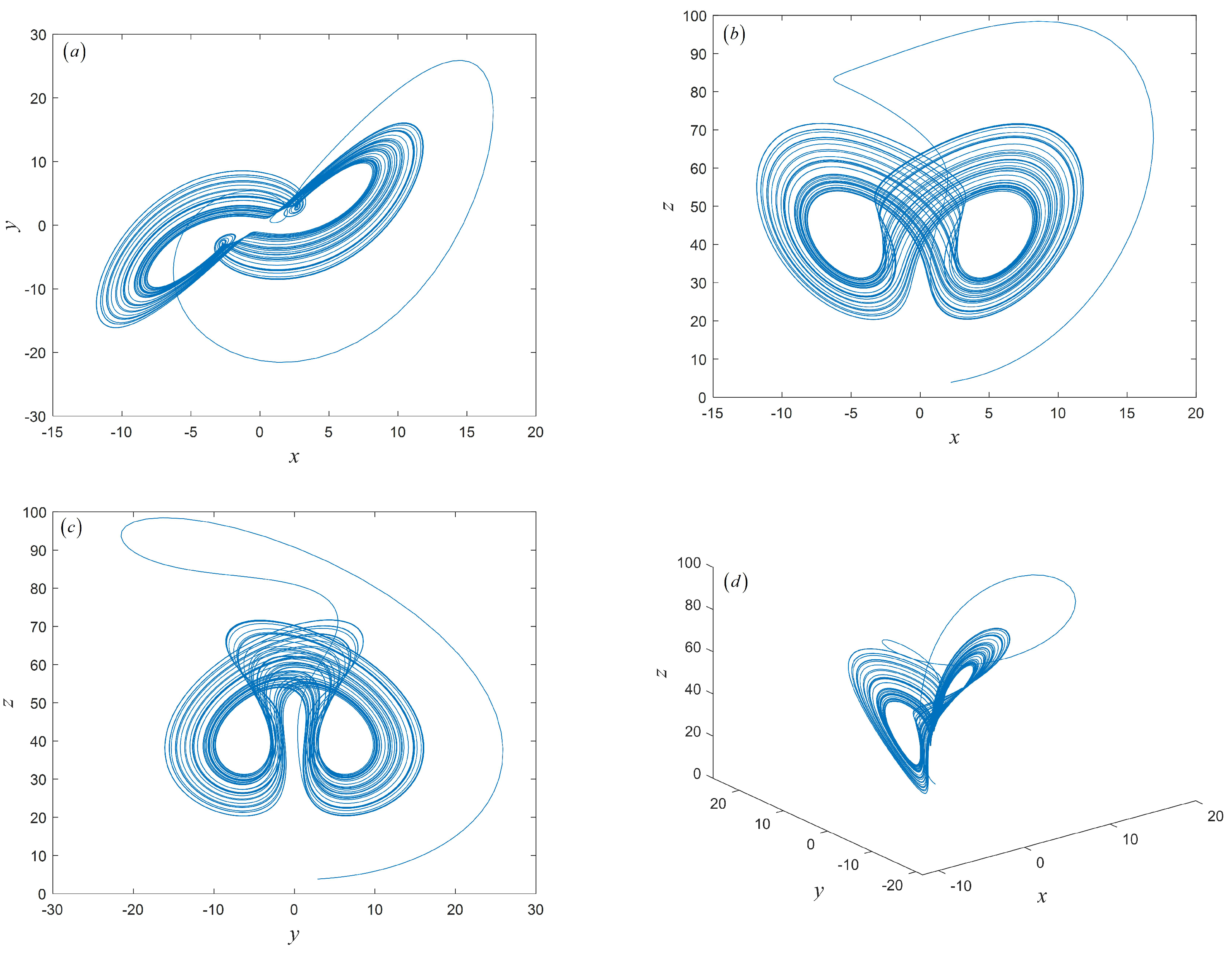
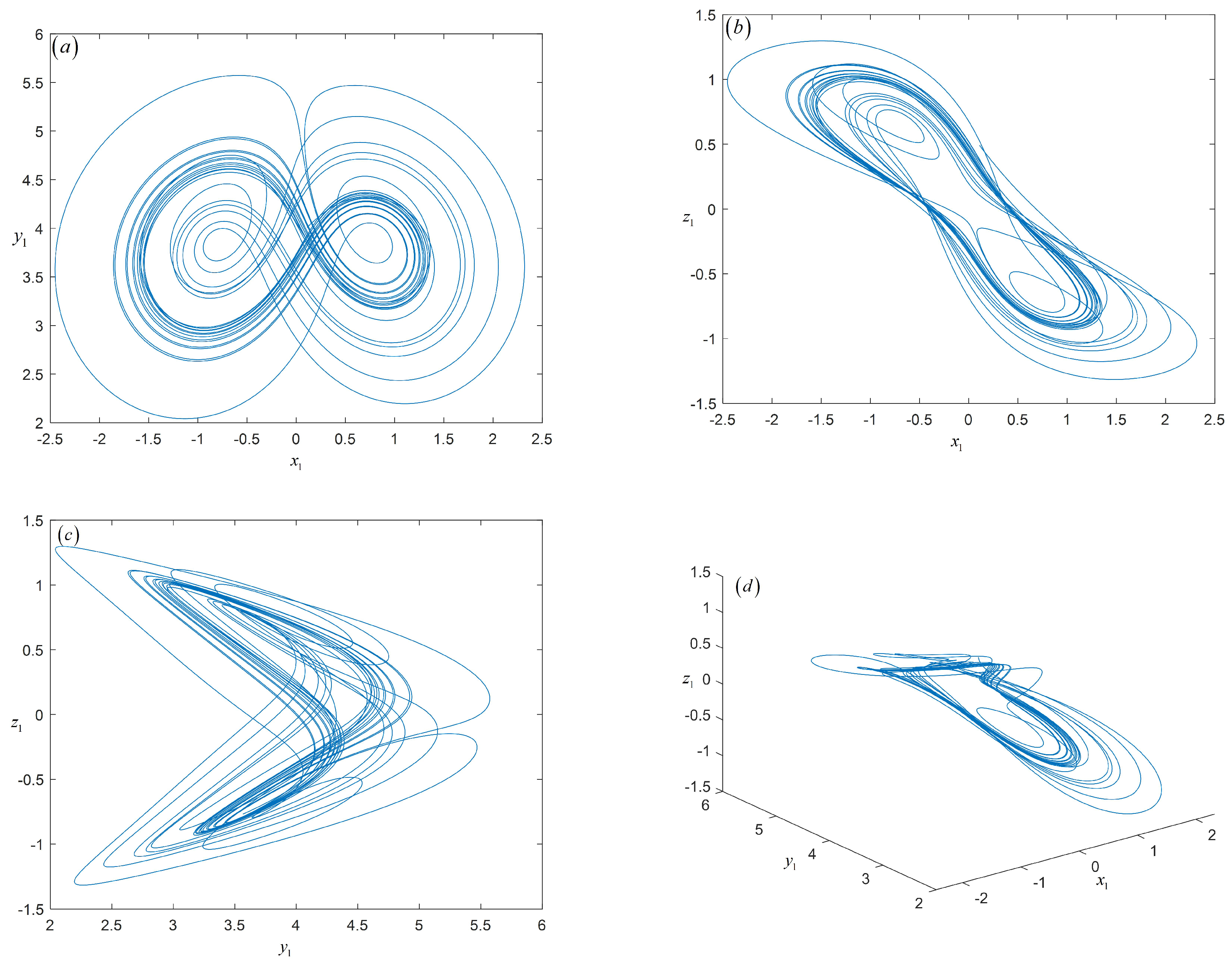
4.1. Fractional-Order Time-Delay Chaotic System

The expression of the fractional delay Liu system [34] is as follows:

$$\left\{\begin{array}{cc}\hfill D_t^{\alpha }x& =a\left(y\right(t)-x(t-\tau \left)\right)\hfill \\ \hfill D_t^{\alpha }y& =bx(t-\tau )-x\left(t\right)z\left(t\right)\hfill \\ \hfill D_t^{\alpha }z& =cz(t-\tau )-d{x}^2\left(t\right)\hfill \end{array},\right.$$

(32)

when the order of the system iwass set as $\alpha =0.97$, the control parameter $(a,b,c,d)=(10,20,-2.5,4)$, and the time delay $0<\tau \le 0.005$, the system was in a chaotic state. In this paper, time $\tau =0.005$ was selected, the initial value state of the system iwass $(x_0,y_0,z_0)=(2.2,2.4,4.8)$, and the phase–space trajectory of the system is shown in Figure 1. The expression of the fractional delay financial system [35] is as follows:

$$\left\{\begin{array}{cc}\hfill D_t^{\alpha }{x}_1& =z_1-a_1{z}_1+x_1{y}_1(t-\tau )\hfill \\ \hfill D_t^{\alpha }{y}_1& =1-b_1{y}_1+x^2(t-\tau )\hfill \\ \hfill D_t^{\alpha }{z}_1& =-x_1(t-\tau )-c_1{z}_1\hfill \end{array},\right.$$

(33)

when the order of the system was $\alpha =0.97$, control parameter $(a_1,b_1,c_1)=(3,0.1,1)$, and time delay $\tau =0.001$, the system was in a chaotic state. In this paper, the initial value state of the system was $(x_0,y_0,z_0)=(0.1,4,0.5)$, and the phase–space trajectory of the system is shown in Figure 2.

4.2. Simulation Results

In order to show the correctness and feasibility of the control method presented in this paper, the fractional delay Lu and financial system with uncertain terms and external disturbances were selected for numerical experiments. The expression of the driving system is as follows:

$$\begin{array}{cc}\hfill D_t^{\alpha }x& =f(x,x(t-{\tau }_2))+\Delta f_1\left(x\right)+d_1\left(t\right)\hfill \\ \hfill & =\left[\begin{array}{c}a(x_2\left(t\right)-x_1(t-{\tau }_1))\hfill \\ b{x}_1(t-{\tau }_1)-x_1\left(t\right)x_3\left(t\right)\hfill \\ c{x}_3(t-{\tau }_1)-d{x}_1^2\left(t\right)\hfill \end{array}\right]+\left[\begin{array}{c}ecos\left(\pi t\right)x_1\\ ecos\left(\pi t\right)x_2\\ ecos\left(\pi t\right)x_3\end{array}\right]+\left[\begin{array}{c}fsin\left(t\right)\\ fsin\left(t\right)\\ fsin\left(t\right)\end{array}\right]\hfill \end{array},$$

(34)

and the expression of the response system is as follows:

$$\begin{array}{cc}\hfill D_t^{\alpha }y& =g(x,x(t-{\tau }_2))+\Delta f_2\left(x\right)+d_2\left(t\right)+U\left(t\right)\hfill \\ \hfill & =\left[\begin{array}{c}{y}_3-a_1{y}_1+y_1{y}_2(t-{\tau }_2)\hfill \\ 1-b_1{y}_2-y_1^2(t-{\tau }_2)\hfill \\ -y_1(t-{\tau }_2)-c_1{y}_3\left(t\right)\hfill \end{array}\right]+\left[\begin{array}{c}{d}_{1}sin\left(\pi t\right)y_1\\ d_{1}sin\left(\pi t\right)y_2\\ d_{1}sin\left(\pi t\right)y_3\end{array}\right]+\left[\begin{array}{c}{f}_{1}cos\left(t\right)\\ f_{1}cos\left(t\right)\\ f_{1}cos\left(t\right)\end{array}\right]+\left[\begin{array}{c}{u}_1\left(t\right)\\ u_2\left(t\right)\\ u_3\left(t\right)\end{array}\right].\hfill \end{array}$$

(35)

From Equations (19), (34) and (35), the synchronization error system is as follows:

$$\left[\begin{array}{c}{\rho }_1-{\widetilde{W_1}}^{T}H-k_{1}sign\left(p{D}_t^{\alpha -1}{e}_1\left(t\right)\right)+q{D}_t^{\alpha -1}{e}_1\left(t\right)\hfill \\ {\rho }_2-{\widetilde{W_2}}^{T}H-k_{2}sign\left(p{D}_t^{\alpha -1}{e}_2\left(t\right)\right)+q{D}_t^{\alpha -1}{e}_2\left(t\right)\hfill \\ {\rho }_3-{\widetilde{W_3}}^{T}H-k_{3}sign\left(p{D}_t^{\alpha -1}{e}_3\left(t\right)\right)+q{D}_t^{\alpha -1}{e}_3\left(t\right)\hfill \end{array}\right].$$

(36)

From Proposition 2, driving system Equation (34) and response system Equation (35) could be synchronized under the action of the controller. The remaining unknown parameters selected in this paper were $e=0.7$, $f=1.3$, $e_1=0.2$, and $f_1=0.5$, and the input variables of the RBF neural network were synchronization error vectors $e_1,e_2,e_3$. The number of hidden layer neurons was 8, and the central matrix of the neurons was as follows:

$$C=\left[\begin{array}{cccccccc}-1.5& 1& -0.5& 0& 0.5& 1& 1.5& 2\\ -1.5& 1& -0.5& 0& 0.5& 1& 1.5& 2\\ -1.5& 1& -0.5& 0& 0.5& 1& 1.5& 2\end{array}\right].$$

(37)

The width value was $b_j=3,(j=1,2,\cdots ,8)$, and the adaptive adjustment parameters were ${\lambda }_i=3000,{\gamma }_i=3.5,(i=1,2,3)$. The initial weights of the neural network were 8 zero vectors, and the initial values of the adaptive law were $k_i\left(0\right)=0.4,(i=1,2,3)$. The values of p and q were $p=0.9,q=-10$. The time step was $h=0.001$ for the numerical simulation. Figure 3a shows that the synchronization error converged quickly, indicating that the designed RBF neural network had a good approximation effect. Figure 3b–d show that each state synchronized well. Figure 4 shows that the amplitude of the weight of the RBF neural network was not large, and the change was relatively stable, which indicates that the control effect of the synchronous controller presented in this paper was better.

5. Conclusions

An adaptive RBF neural network controller and an integer-order parameter adaptive law were presented for the synchronization of a heterogeneous structured fractional-order chaotic system with completely unknown nonlinear uncertainties and external disturbances. The controller and the RBF neural network were combined with adaptive control technology. On the one hand, the unknown nonlinear function was approximated with an RBF neural network. On the other hand, an adaptive law was used to adjust the corresponding parameters in the controller. Numerical simulation results show that the controller designed in this paper not only realized the synchronization control of heterogeneous structure fraction-order time-delay chaotic systems, but also had fast response speed, a good control effect, and strong anti-interference ability. In future work, we will construct a secure communication scheme on the basis of this synchronization scheme that forms an encrypted signal by driving the sequence generated by the system and the signal to be encrypted, the decryptor decrypts the encrypted signal in response to the sequence generated by the system, and the recovered signal is obtained. Therefore, the results of this study are not only of great theoretical importance, but also have great application value in the field of secure communication.

References

1. Rakkiyappan, R.; Chandrasekar, A.; Lakshmanan, S. Effects of leakage time-varying delays in Markovian jump neural networks with impulse control. Neurocomputing 2013, 121, 365–378. [Google Scholar] [CrossRef]
2. Rakkiyappan, R.; Chandrasekar, A.; Lakshmanan, S. Exponential stability of Markovian jumping stochastic Cohen-Grossberg neural networks with mode-dependent probabilistic time-varying delays and impulses. Neurocomputing 2014, 131, 265–277. [Google Scholar] [CrossRef]
3. Li, T.; Wang, T.; Song, A.; Fei, S. Combined convex technique on delay-dependent stability for delayed neural networks. IEEE Trans. Neural Netw. Learn. Syst. 2013, 24, 1459–1466. [Google Scholar] [CrossRef] [PubMed]
4. Deng, Y.M.; Fan, H.F.; Wu, S.M. A hybrid ARIMA-LSTM model optimized by BP in the forecast of outpatient visits. J. Ambient Intell. Humaniz. Comput. 2020. [Google Scholar] [CrossRef]
5. Deng, W.; Li, C.; Lu, J. Stability analysis of linear fractional differential system with multiple time delays. Nonlinear Dyn. 2007, 48, 409–416. [Google Scholar] [CrossRef]
6. Xiao, M.; Zheng, W.; Cao, J. Bifurcation and control in a neural network with small and large delays. Neural Netw. 2013, 44, 132–142. [Google Scholar] [CrossRef]
7. Choi, S.W.; Kim, B.H.S. Applying PCA to Deep Learning Forecasting Models for Predicting PM2.5. Sustainability 2021, 13, 3726. [Google Scholar] [CrossRef]
8. Xiao, D.Y.; Su, J.X. Research on Stock Price Time Series Prediction Based on Deep Learning and Autoregressive Integrated Moving Average. Sci. Program.-Neth. 2022, 2022, 4758698. [Google Scholar] [CrossRef]
9. Aghababa, M. Control of fractional-order systems using chatter-free sliding mode approach. J. Comput. Nonlinear Dyn. 2014, 9, 031003. [Google Scholar] [CrossRef]
10. Aghababa, M. No-chatter variable structure control for fractional nonlinear complex systems. Nonlinear Dyn. 2013, 73, 2329–2342. [Google Scholar] [CrossRef]
11. Aghababa, M. Synchronization and stabilization of fractional second-order nonlinear complex systems. Nonlinear Dyn. 2015, 80, 1731–1744. [Google Scholar] [CrossRef]
12. Pecora, L.; Carroll, T. Synchronization in chaotic system. Phys. Rev. Lett. 1990, 64, 821–824. [Google Scholar] [CrossRef] [PubMed]
13. Megherbi, O.; Hamiche, H.; Djennoune, S. A New Contribution for the Impulsive Synchronization of Fractional-Order Discrete-Time Chaotic Systems. Nonlinear Dyn. 2017, 980, 1519–1533. [Google Scholar] [CrossRef]
14. Park, J.H. Adaptive modified projective synchronization of a unified chaotic system with an uncertain parameter. Chaos Solitons Fractals 2017, 34, 1552–1559. [Google Scholar] [CrossRef]
15. Mobayen, S. Chaos Synchronization of Uncertain Chaotic Systems Using Composite Nonlinear Feedback Based Integral Sliding Mode Control. ISA Trans. 2018, 77, 100–111. [Google Scholar] [CrossRef] [PubMed]
16. Sangyun, L.; Mignon, P.; Jaeho, B. Robust adaptive synchronization of a class of chaotic systems via fuzzy bilinear observer using projection operator. Inf. Sci. 2017, 402, 182–198. [Google Scholar]
17. Chou, H.; Chuang, C.; Wang, W. A Fuzzy-Model-Based Chaotic Synchronization and Its Implementation on a Secure Communication System. IEEE Trans. Inf. Forensics Secur. 2013, 8, 2177–2185. [Google Scholar] [CrossRef]
18. Xu, G.; Xu, J.; Xiu, C.; Liu, F.; Zang, Y. Secure communication based on the synchronous control of hysteretic chaotic neuron. Neurocomputing 2017, 227, 108–112. [Google Scholar] [CrossRef]
19. Mainieri, R.; Rehacek, J. Projective synchronization in three-dimensional chaotic systems. Phys. Rev. Lett. 1999, 82, 3024–3045. [Google Scholar] [CrossRef]
20. Velmurugan, G.; Rakkiyappan, R. Hybrid Projective Synchronization of Fractional-Order Chaotic Complex Nonlinear Systems with Time Delays. J. Comput. Nonlinear Dyn. 2016, 11, 031016. [Google Scholar] [CrossRef]
21. Wang, S.; Yu, Y.; Wen, G. Hybrid projective synchronization of time-delayed fractional order chaotic systems. Nonlinear-Anal.-Hybrid Syst. 2014, 11, 129–138. [Google Scholar] [CrossRef]
22. Wang, X.Y.; He, Y.J. Projective synchronization of fractional order chaotic system based on linear separation. Phys. Lett. A 2008, 372, 435–441. [Google Scholar] [CrossRef]
23. Bao, H.B.; Cao, J. Projective synchronization of fractional-order memristor-based neural networks. Neural Netw. 2015, 63, 1–9. [Google Scholar] [CrossRef]
24. Zhou, P.; Zhu, W. Function projective synchronization for fractional-order chaotic systems. Nonlinear Anal. Real World Appl. 2011, 12, 811–816. [Google Scholar] [CrossRef]
25. Chen, J.; Zeng, Z.; Jiang, P. Global Mittag–Leffler stability and synchronization of memristor-based fractional-order neural networks. Neural Netw. 2014, 51, 1–8. [Google Scholar] [CrossRef]
26. Wang, X.Y.; Zhang, X.P.; Ma, C. Modified projective synchronization of fractional-order chaotic systems via active sliding mode control. Nonlinear Dyn. 2012, 69, 511–517. [Google Scholar] [CrossRef]
27. Yu, J.; Hu, C.; Jiang, H.; Fan, X. Projective synchronization for fractional neural networks. Neural Netw. 2014, 49, 87–95. [Google Scholar] [CrossRef]
28. Wang, S.; Yu, Y.G.; Diao, M. Hybrid projective synchronization of chaotic fractional order systems with different dimensions. Phys. A 2010, 389, 4981–4988. [Google Scholar] [CrossRef]
29. Wu, R.C.; Hei, X.D.; Chen, L.P. Finite-time stability of fractional-order neural networks with delay. Commun. Theor. Phys. 2013, 60, 189–193. [Google Scholar] [CrossRef]
30. Lazarevic, M.; Debeljkovic, D. Finite time stability analysis of linear autonomous fractional order systems with delayed state. Asian J. Control 2005, 7, 440–447. [Google Scholar] [CrossRef]
31. Lazarevic, M.; Spasic, A. Finite-time stability analysis of fractional order time-delay systems: Gronwall’s approach. Math. Comput. Model. 2009, 49, 475–481. [Google Scholar] [CrossRef]
32. Lorenz, C.; Hartley, T. Variable order and distributed order fractional operators. Nonlinear Dyn. 2002, 29, 57–98. [Google Scholar] [CrossRef]
33. Samko, S.; Kilbas, A.; Marichev, O. Fractional Integrals and Derivatives; Gordon and Breach Science Publishers: Basel, Switzerland, 1993. [Google Scholar]
34. Gorenflo, R.; Mainardi, F. Fractional Calculus; Springer: New York, NY, USA, 1997. [Google Scholar]
35. Liu, H.; Pan, Y.; Li, S. Adaptive fuzzy backstepping control of fractional-order nonlinear systems. IEEE Trans. Syst. Man Cybern. Syst. 2017, 47, 2209–2217. [Google Scholar] [CrossRef]
Figure 1. Phase–space trajectory distribution of fractional delay financial system: (a) X–Y plane; (b) X–Z plane; (c) Y–Z plane; (d) X–Y–Z plane.
Fractalfract 07 00288 g001
Figure 2. Phase–space trajectory distribution of fractional delay Liu system: (a) X–Y plane; (b) X–Z plane; (c) Y–Z plane; (d) X–Y–Z plane.
Fractalfract 07 00288 g002
Figure 3. State trajectories of synchronization error vectors (a) e 1 , e 2 ,and e 3 , (b) x 1 and y 1 , (c) x 2 and y 2 , and (d) x 3 and y 3 .
Fractalfract 07 00288 g003
Figure 4. The optimal weight value of the neural network.
Fractalfract 07 00288 g004
Disclaimer/Publisher’s Note: The statements, opinions and data contained in all publications are solely those of the individual author(s) and contributor(s) and not of MDPI and/or the editor(s). MDPI and/or the editor(s) disclaim responsibility for any injury to people or property resulting from any ideas, methods, instructions or products referred to in the content.