Bifurcation Phenomenon and Control Technique in Fractional BAM Neural Network Models Concerning Delays

Abstract

In this current study, we formulate a kind of new fractional BAM neural network model concerning five neurons and time delays. First, we explore the existence and uniqueness of the solution of the formulated fractional delay BAM neural network models via the Lipschitz condition. Second, we study the boundedness of the solution to the formulated fractional delayed BAM neural network models using a proper function. Third, we set up a novel sufficient criterion on the onset of the Hopf bifurcation stability of the formulated fractional BAM neural network models by virtue of the stability criterion and bifurcation principle of fractional delayed dynamical systems. Fourth, a delayed feedback controller is applied to command the time of occurrence of the bifurcation and stability domain of the formulated fractional delayed BAM neural network models. Lastly, software simulation figures are provided to verify the key outcomes. The theoretical outcomes obtained through this exploration can play a vital role in controlling and devising networks.

1. Introduction

Recently, the investigation of neural network models has aroused much interest from many scholars due to the wide application of neural networks in many areas, such as image processing, artificial intelligence, automatic control, associative memories, parallel computation, biological engineering, disease diagnosis, and more [1,2,3,4,5]. All these applications rely on the dynamics of neural network models; thus, the study of various dynamic behaviors of neural networks has attracted great attention in the scientific community. During the past several decades, a great deal of valuable results have been gained on neural networks. For example, Li and Shen [6] dealt with the near-automorphic solution to Clifford-valued delayed fuzzy cellular neural networks; Xu et al. [7] investigated the pseudo-near-periodic oscillation to quaternion-valued fuzzy delayed neural network models; Cui et al. [8] carried out a detailed analysis on fixed-time synchronization in a kind of Markovian jump fuzzy stochastic delayed neural network models; and Huang et al. [9] explored the anti-periodic oscillation to delayed neural network models. For more related studies, interested readers can refer to [10,11,12,13,14,15].

Here, we would to point out that all the publications above are concerned merely with the integer-order neural networks with delays. Now, the fractional-order dynamical model has displayed great application in numerous areas, including various aspects of waves, mechanics, control science, biology, neural networks, finance, information security, and more [16,17,18,19,20]. The present investigation indicates that fractional-order differential equations are a more effective tool to describe phenomena in the real world than integer-order ones, as fractional-order differential equations are able to retain memory and heredity for many dynamic development processes [21,22,23,24]. Recently, a great deal of valuable results on fractional-order dynamical systems have been presented. In particular, many excellent works on fractional delayed neural networks have been achieved. For example, Ci et al. [25] explored multiple asymptotical $\omega$-periodicity in fractional-order neural networks concerning delays; Lin et al. [26] discussed output synchronization and PD control of a kind of coupled fractional-order neural network models involving delays; Xiao et al. [27] performed a meaningful study for a new controller design of finite-time synchronization in fractional memristive neural networks; and Zhang et al. [28] set up a sufficient condition to ensure the global Mittag-Leffler synchronization in discrete-time fractional-order delayed neural networks. For further details, see [29,30,31,32].

Periodic oscillation is a vital dynamic behavior of delayed neural networks. In particular, delay-driven Hopf bifurcation can be regarded as a special form of periodic oscillation. Delay-driven Hopf bifurcation in neural networks plays an important role in their design. Thus, delay-driven Hopf bifurcation of neural networks has attracted much interest from many researchers. During the past several decades, many scholars have made great efforts to explore delay-driven Hopf bifurcation for various delayed neural networks. However, they have only paid serious attention to integer-order delayed neural network models. The research on delay-driven Hopf bifurcation of fractional delayed neural network models is relatively scarce. At present, there exist a few publications on this topic. For example, Huang et al. [33] discussed the impact of time delay on Hopf bifurcation in a class of delayed fractional quaternion-valued neural network models; Xu et al. [34] analyzed delay-driven Hopf bifurcation in fractional delayed BAM neural network models with multiple delays; and Huang et al. [35] set up a novel bifurcation result for fractional BAM neural networks involving leakage-type time delay. Kaslik and Rădulescu [36] discussed the Hopf bifurcation and stability behavior of fractional gene regulation network models. For further details, refer to [37,38,39,40].

Several researchers have studied the delay-driven Hopf bifurcation issue in fractional neural network models; however, there exist numerous open questions yet to be handled. Unlike integer-order neural network models, fractional delayed neural network models possess one more coefficient (e.g., fractional order), making the characteristic equation more complex. Thus, how to reveal the dynamics of fractional-order delayed neural networks is a vital aspect. Stimulated by this idea, in the current investigation we explore the following themes: (1) We test the existence, uniqueness, and boundedness of a solution to fractional BAM neural network models with time delays; (2) We construct a criterion guaranteeing the onset of Hopf bifurcation and the stability of a fractional BAM neural network model with time delays; (3) We investigate the influence of time delay on Hopf bifurcation and the stability of fractional BAM neural network models with time delays.

In 2009, Yang and Ye [41] investigated the following BAM neural network models with two different delays:

$$\left\{\begin{array}{c}{\displaystyle {\dot{y}}_1\left(t\right)=-a_1{y}_1\left(t\right)+b_{21}{g}_1\left(y_2(t-{\vartheta }_2)\right)+b_{31}{g}_1\left(y_3(t-{\vartheta }_2)\right)}\hfill \\ {\displaystyle +b_{41}{g}_1\left(y_4(t-{\vartheta }_2)\right)+b_{51}{g}_1\left(y_5(t-{\vartheta }_2)\right),}\hfill \\ {\displaystyle {\dot{y}}_2\left(t\right)=-a_2{y}_2\left(t\right)+b_{12}{g}_2\left(y_1(t-{\vartheta }_1)\right),}\hfill \\ {\displaystyle {\dot{y}}_3\left(t\right)=-a_3{y}_3\left(t\right)+b_{13}{g}_3\left(y_1(t-{\vartheta }_1)\right),}\hfill \\ {\displaystyle {\dot{y}}_4\left(t\right)=-a_4{y}_4\left(t\right)+b_{14}{g}_4\left(y_1(t-{\vartheta }_1)\right),}\hfill \\ {\displaystyle {\dot{y}}_5\left(t\right)=-a_5{y}_5\left(t\right)+b_{15}{g}_5\left(y_1(t-{\vartheta }_1)\right),}\hfill \end{array}\right.$$

(1)

where $y_k(k=1,2,3,4,5)$ represents the state of the kth neuron, $a_i>0$ $(i=1,2,3,4,5)$ represents the stability trait of the treatment of interior neurons lying on two layers, $b_{k1}$ $(k=2,3,4,5)$, and $b_{1j} (j=2,3,4,5)$ implies the connect weights through two layers. Here, $g_i (i=1,2,3,4,5)$ implies the activation function, while ${\vartheta }_1,{\vartheta }_2$ are delays. For more details, see [41]. Taking advantage of an appropriate variable substitution, Yang and Ye [41] modified system (1) as an isovalent expression and then carried out a circumstantial discussion of the bifurcation phenomenon with respect to system (1).

Relying on exploration of Yang and Ye [41] and the discussion above, we modify system (1) as the following fractional case:

$$\left\{\begin{array}{c}{\displaystyle \frac{d^p{y}_1\left(t\right)}{d{t}^p}=-a_1{y}_1\left(t\right)+b_{21}{g}_1\left(y_2(t-{\vartheta }_2)\right)+b_{31}{g}_1\left(y_3(t-{\vartheta }_2)\right)}\hfill \\ {\displaystyle +b_{41}{g}_1\left(y_4(t-{\vartheta }_2)\right)+b_{51}{g}_1\left(y_5(t-{\vartheta }_2)\right),}\hfill \\ {\displaystyle \frac{d^p{y}_2\left(t\right)}{d{t}^p}=-a_2{y}_2\left(t\right)+b_{12}{g}_2\left(y_1(t-{\vartheta }_1)\right),}\hfill \\ {\displaystyle \frac{d^p{y}_3\left(t\right)}{d{t}^p}=-a_3{y}_3\left(t\right)+b_{13}{g}_3\left(y_1(t-{\vartheta }_1)\right),}\hfill \\ {\displaystyle \frac{d^p{y}_4\left(t\right)}{d{t}^p}=-a_4{y}_4\left(t\right)+b_{14}{g}_4\left(y_1(t-{\vartheta }_1)\right),}\hfill \\ {\displaystyle \frac{d^p{y}_5\left(t\right)}{d{t}^p}=-a_5{y}_5\left(t\right)+b_{15}{g}_5\left(y_1(t-{\vartheta }_1)\right),}\hfill \end{array}\right.$$

(2)

where $p\in (0,1]$ is a constant. The remaining functions and parameters have connotations identical to those in model (1). Model (2) and model (1) possess the same equilibrium point. The initial condition of model (2) is presented as follows:

$$\left\{\begin{array}{c}{\displaystyle y_1\left(\phi \right)=y_{1\phi },}\hfill \\ {\displaystyle y_2\left(\phi \right)=y_{2\phi },}\hfill \\ {\displaystyle y_3\left(\phi \right)=y_{3\phi },}\hfill \\ {\displaystyle y_4\left(\phi \right)=y_{4\phi },}\hfill \\ {\displaystyle y_5\left(\phi \right)=y_{5\phi },}\hfill \end{array}\right.$$

(3)

where $t_0$ is a positive constant and $\phi \in [-\vartheta ,t_0]$. For the sake of convenience, we make the following assumptions:

$\left({\mathcal{A}}_1\right)$$g_i\in C^1,g_i\left(0\right)=0,i=1,2,3,4,5.$

$\left({\mathcal{A}}_2\right)$ For $h=1,2,3,4,5$, ∃ a constant $G_h>0$ obeying $|g_h\left({\iota }_1\right)-g_i\left({\iota }_2\right)|\le G_h|{\iota }_1-{\iota }_2|,$∀ ${\iota }_1,{\iota }_2\in R.$

$\left({\mathcal{A}}_3\right)$ For $h=1,2,3,4,5$, ∃ a constant $M_h>0$ obeying $|g_h\left(\iota \right)|\le M_h,$∀ $\iota \in R.$

$\left({\mathcal{A}}_4\right)$${\vartheta }_1+{\vartheta }_2=\vartheta$.

The framework of the rest of this study is as follows. In Section 2 we recall several related lemmas and definitions about fractional-order differential equations. Section 3 proves the uniqueness and existence of the solution to model (2). Section 4 proves the boundedness of the solution to model (2). Section 5 is concerned with the appearance of Hopf bifurcation and the stability of model (2). Section 6 controls the bifurcation behavior of model (2) using a delayed feedback controller. Section 7 carries out software simulations to check the key outcomes of this exploration. Finally, Section 8 ends this study.

2. Preliminaries

In this segment, several necessary lemmas and definitions about fractional differential equations are prepared. Label $R_{+}=\left\{x\right|x\ge 0,x\in R\}$.

Definition 1

([42]). We define a Caputo-type fractional derivative as follows:

$${\mathcal{D}}^{p}f\left(\varsigma \right)=\frac{1}{\mathsf{\Gamma }(\kappa -p)}{\int }_{{\varsigma }_0}^{\varsigma }\frac{f^{\left(\kappa \right)}\left(s\right)}{{(\varsigma -s)}^{p-\kappa +1}}ds,$$

where $f\left(\varsigma \right)\in ([{\varsigma }_0,\infty ),R),\mathsf{\Gamma }\left(t\right)={\int }_0^{\infty }{\varsigma }^{t-1}{e}^{-\varsigma }d\varsigma ,$ $\varsigma \ge {\varsigma }_0$ and $\kappa \in Z^{+},\kappa -1\le p<\kappa .$

We provide the Laplace transform of a Caputo-type fractional derivative as follows:

$$\mathcal{L}\{{\mathcal{D}}^{p}f\left(t\right);s\}=s^p\mathcal{F}\left(s\right)-\sum _{j=0}^{m-1}{s}^{p-j-1}{f}^{\left(j\right)}\left(0\right),m-1\le p<m\in Z^{+},$$

where $\mathcal{F}\left(s\right)=\mathcal{L}\left\{f\right(t\left)\right\}.$ In particular, if $f^{\left(j\right)}\left(0\right)=0, j=1,2,\cdots ,n,$ then $\mathcal{L}\{{\mathcal{D}}^{p}f\left(t\right);s\}=s^p\mathcal{F}\left(s\right).$

Definition 2

([43]). $(y_{1*},y_{2*},y_{3*},y_{4*},y_{5*})$ is called an equilibrium point of system (2) if

$$\left\{\begin{array}{c}{\displaystyle -a_1{y}_{1*}+b_{21}{g}_1\left(y_{2*}\right)+b_{31}{g}_1\left(y_{3*}\right)+b_{41}{g}_1\left(y_{4*}\right)+b_{51}{g}_1\left(y_{5*}\right)=0,}\hfill \\ {\displaystyle -a_2{y}_{2*}+b_{12}{g}_2\left(y_{1*}\right)=0,}\hfill \\ {\displaystyle -a_3{y}_{3*}+b_{13}{g}_3\left(y_{1*}\right)=0,}\hfill \\ {\displaystyle -a_4{y}_{4*}+b_{14}{g}_4\left(y_{1*}\right)=0,}\hfill \\ {\displaystyle -a_5{y}_{5*}+b_{15}{g}_5\left(y_{1*}\right)=0}\hfill \end{array}\right.$$

(4)

Lemma 1

([44]). Consider the following system:

$${\displaystyle \frac{d^{p}u\left(t\right)}{d{t}^p}=f(t,u\left(t\right)),u\left(t_0\right)=u_{t_0},}$$

(5)

where $t_0$ is a positive real number, $p\in (0,1],f:[t_0,\infty )\times \omega \to R_{+}^n,\omega \subset R_{+}^n$. If $f(t,u)$ obeys the Lipschitz condition concerning u, then system (5) admits a unique solution that is defined on $[t_0,\infty ).$

Lemma 2

([45]). Let $u\left(t\right)\in [t_0,\infty )$, which obeys

$$\left\{\begin{array}{c}{\displaystyle D^{p}u\left(t\right)\le -{\sigma }_{1}u\left(t\right)+{\sigma }_2,}\hfill \\ {\displaystyle u\left(t_0\right)=u_{t_0},}\hfill \end{array}\right.$$

(6)

where $0<p<1,{\sigma }_1,{\sigma }_2\in R,{\sigma }_1\ne 0,t_0\ge 0$. Then,

$$u\left(t\right)\le \left(u\left(t_0\right)-\frac{{\sigma }_2}{{\sigma }_1}\right)E_p[-{\sigma }_1{(t-t_0)}^p]+\frac{{\sigma }_2}{{\sigma }_1},$$

(7)

where $E_p$ is one-parameter form of Mittag-Leffler function and is given by

$$E_p\left(y\right)=\sum _{\varpi =0}^{\infty }\frac{y^{\varpi }}{\mathsf{\Gamma }(p\varpi +1)},p>0,$$

where y denotes a complex number.

Lemma 3

([46,47]). For the system as follows

$${\displaystyle \frac{d^{p}v\left(t\right)}{d{t}^p}=f(t,v\left(t\right)),v\left(0\right)=v_0,}$$

(8)

where $p\in (0,1]$ and $f(t,v\left(t\right)):R^{+}\times R^n\to R^n$. The steady state of system (8) keeps locally asymptotically stability if all eigenvalues ω of $\frac{\partial f(t,v)}{\partial v}$ evaluated near the steady state obey $\left|arg\left(\omega \right)\right|>\frac{p\pi }{2}$.

Lemma 4

([48]). For the system as follows:

$$\left\{\begin{array}{c}{\displaystyle \frac{d^{p_1}{\mathcal{Y}}_1\left(t\right)}{d{t}^{p_1}}=f_{11}{\mathcal{Y}}_1(t-{\vartheta }_{11})+f_{12}{\mathcal{Y}}_2(t-{\vartheta }_{12})+\cdots +f_{1n}{\mathcal{Y}}_n(t-{\vartheta }_{1n}),}\hfill \\ {\displaystyle \frac{d^{p_2}{\mathcal{Y}}_2\left(t\right)}{d{t}^{p_2}}=f_{21}{\mathcal{Y}}_1(t-{\vartheta }_{21})+f_{22}{\mathcal{Y}}_2(t-{\vartheta }_{22})+\cdots +f_{2n}{\mathcal{Y}}_n(t-{\vartheta }_{2n}),}\hfill \\ {\displaystyle ⋮}\hfill \\ {\displaystyle \frac{d^{p_n}{\mathcal{Y}}_n\left(t\right)}{d{t}^{p_n}}=f_{n1}{\mathcal{Y}}_1(t-{\vartheta }_{n1})+f_{n2}{\mathcal{Y}}_2(t-{\vartheta }_{n2})+\cdots +f_{nn}{\mathcal{Y}}_n(t-{\vartheta }_{nn}),}\hfill \end{array}\right.$$

(9)

where $0<p_j<1 (j=1,2,\cdots ,n)$, the initial values ${\mathcal{Y}}_k\left(t\right)={\varpi }_k\left(t\right)\in C[-{max}_{k,l}{\vartheta }_{kl},0],$ $t\in [-{max}_{k,l}{\vartheta }_{kl},0],$ $k, l=1,2,\cdots ,n.$ Let

$$\Delta \left(\varrho \right)=\left[\begin{array}{cccc}{\varrho }^{p_1}-f_{11}{e}^{-\varrho {\vartheta }_{11}}& -f_{12}{e}^{-\varrho {\vartheta }_{12}}& \cdots & -f_{1n}{e}^{-\varrho {\vartheta }_{1n}}\\ -f_{21}{e}^{-\varrho {\vartheta }_{12}}& {\varrho }^{p_2}-f_{22}{e}^{-\varrho {\vartheta }_{22}}& \cdots & -f_{2n}{e}^{-\varrho {\vartheta }_{2n}}\\ ⋮& ⋮& \ddots & ⋮\\ -f_{n1}{e}^{-\varrho {\vartheta }_{n1}}& -f_{n2}{e}^{-\varrho {\sigma }_{n2}}& \cdots & {\zeta }^{p_n}-f_{nn}{e}^{-\varrho {\vartheta }_{nn}}\end{array}\right],$$

(10)

then, the null solution of Equation (9) keeps Lyapunov asymptotic stability if the real part of every root of $det(\Delta (\varrho \left)\right)=0$ is negative.

3. Existence and Uniqueness

Theorem 1.

Set $\mathsf{\Omega }=\{(y_1,y_2,y_3,y_4,y_5)\in R^5:max\left\{\right|y_1|,|y_2|,|y_3|,|y_4|,|y_5\left|\right\}<\mathcal{A}\}$, where $\mathcal{A}>0$ denotes a constant. Then, for every ${\mathcal{Y}}_{t_0}=(y_{1t_0},y_{2t_0},y_{3t_0},y_{4t_0},y_{5t_0})\in \mathsf{\Omega }$ and for every $t\ge t_0$ there admits a unique solution $\mathcal{Y}\left(t\right)\in \mathsf{\Omega }$ of model (2) involving the initial condition ${\mathcal{Y}}_{t_0}$.

Proof. 

We need to prove the existence and uniqueness of the solution to model (2) based on the domain $\mathsf{\Omega }\times [t_0,t_{01}],$ where $t_{01}<+\infty .$ We denote $\mathcal{Y}=(y_1,y_2,y_3,y_4,y_5)$ and $\tilde{\mathcal{Y}}=({\tilde{y}}_1,{\tilde{y}}_2,{\tilde{y}}_3,{\tilde{y}}_4,{\tilde{y}}_5)$ and define the following mapping: $\mathsf{\Gamma }\left(\mathcal{Y}\right)=({\mathsf{\Gamma }}_1\left(\mathcal{Y}\right),{\mathsf{\Gamma }}_2\left(\mathcal{Y}\right),{\mathsf{\Gamma }}_3\left(\mathcal{Y}\right),{\mathsf{\Gamma }}_4\left(\mathcal{Y}\right),{\mathsf{\Gamma }}_5\left(\mathcal{Y}\right))$, where

$$\left\{\begin{array}{c}{\displaystyle {\mathsf{\Gamma }}_1\left(\mathcal{Y}\right)=-a_1{y}_1\left(t\right)+b_{21}{g}_1\left(y_2(t-{\vartheta }_2)\right)+b_{31}{g}_1\left(y_3(t-{\vartheta }_2)\right)}\hfill \\ {\displaystyle +b_{41}{g}_1\left(y_4(t-{\vartheta }_2)\right)+b_{51}{g}_1\left(y_5(t-{\vartheta }_2)\right),}\hfill \\ {\displaystyle {\mathsf{\Gamma }}_2\left(\mathcal{Y}\right)=-a_2{y}_2\left(t\right)+b_{12}{g}_2\left(y_1(t-{\vartheta }_1)\right),}\hfill \\ {\displaystyle {\mathsf{\Gamma }}_3\left(\mathcal{Y}\right)=-a_3{y}_3\left(t\right)+b_{13}{g}_3\left(y_1(t-{\vartheta }_1)\right),}\hfill \\ {\displaystyle {\mathsf{\Gamma }}_4\left(\mathcal{Y}\right)=-a_4{y}_4\left(t\right)+b_{14}{g}_4\left(y_1(t-{\vartheta }_1)\right),}\hfill \\ {\displaystyle {\mathsf{\Gamma }}_5\left(\mathcal{Y}\right)=-a_5{y}_5\left(t\right)+b_{15}{g}_5\left(y_1(t-{\vartheta }_1)\right).}\hfill \end{array}\right.$$

(11)

For arbitrary $\mathcal{Y},\tilde{\mathcal{Y}}\in \Pi$, $t_1,t_2\in R,t_1,t_2\ge t_0$, by $\left({\mathcal{A}}_2\right)$, we have

$$\begin{array}{ccc}& & \left|\right|\mathsf{\Gamma }\left(\mathcal{Y}\right)-\mathsf{\Gamma }\left(\tilde{\mathcal{Y}}\right)\left|\right|\hfill \\ & =& \sum _{l=1}^5|{\mathsf{\Gamma }}_l\left(\mathcal{Y}\right)-{\mathsf{\Gamma }}_l\left(\tilde{\mathcal{Y}}\right)|\hfill \\ & =& \left|\right[-a_1{y}_1\left(t_1\right)+b_{21}{g}_1\left(y_2(t_1-{\vartheta }_2)\right)+b_{31}{g}_1\left(y_3(t_1-{\vartheta }_2)\right)\hfill \\ & & +b_{41}{g}_1\left(y_4(t_1-{\vartheta }_2)\right)+b_{51}{g}_1\left(y_5(t_1-{\vartheta }_2)\right)]\hfill \\ & & -[-a_1{y}_1\left(t_2\right)+b_{21}{g}_1\left(y_2(t_2-{\vartheta }_2)\right)+b_{31}{g}_1\left(y_3(t_2-{\vartheta }_2)\right)\hfill \\ & & +b_{41}{g}_1\left(y_4(t_2-{\vartheta }_2)\right)+b_{51}{g}_1\left(y_5(t_2-{\vartheta }_2)\right)\left]\right|\hfill \\ & & +|[-a_2{y}_2\left(t_1\right)+b_{12}{g}_2\left(y_1(t_1-{\vartheta }_1)\right)]-[-a_2{y}_2\left(t_2\right)+b_{12}{g}_2\left(y_1(t_2-{\vartheta }_1)\right)]|\hfill \\ & & +|[-a_3{y}_3\left(t_1\right)+b_{13}{g}_3\left(y_1(t_1-{\vartheta }_1)\right)]-[-a_3{y}_3\left(t_2\right)+b_{13}{g}_3\left(y_1(t_2-{\vartheta }_1)\right)]|\hfill \\ & & +|[-a_4{y}_4\left(t_1\right)+b_{14}{g}_4\left(y_1(t_1-{\vartheta }_1)\right)]-[-a_4{y}_4\left(t_2\right)+b_{14}{g}_4\left(y_1(t_2-{\vartheta }_1)\right)]|\hfill \\ & & +|[-a_5{y}_5\left(t_1\right)+b_{15}{g}_5\left(y_1(t_1-{\vartheta }_1)\right)]-[-a_5{y}_5\left(t_2\right)+b_{15}{g}_5\left(y_1(t_2-{\vartheta }_1)\right)]|\hfill \\ & \le & a_1|y_1\left(t_1\right)-y_1\left(t_2\right)|+|b_{21}|G_1|y_2(t_1-{\vartheta }_2)-y_2(t_2-{\vartheta }_2)|\hfill \\ & & +|b_{31}|G_1|y_3(t_1-{\vartheta }_2)-y_3(t_2-{\vartheta }_2)|+|b_{41}|G_1|y_4(t_1-{\vartheta }_2)-y_4(t_2-{\vartheta }_2)|\hfill \\ & & +|b_{51}|G_1|y_5(t_1-{\vartheta }_2)-y_5(t_2-{\vartheta }_2)|+a_2|y_2\left(t_1\right)-y_2\left(t_2\right)|\hfill \\ & & +|b_{12}|G_2|y_1(t_1-{\vartheta }_2)-y_1(t_2-{\vartheta }_2)|+a_3|y_3\left(t_1\right)-y_3\left(t_2\right)|\hfill \\ & & +|b_{13}|G_3|y_1(t_1-{\vartheta }_2)-y_1(t_2-{\vartheta }_2)|+a_4|y_4\left(t_1\right)-y_4\left(t_2\right)|\hfill \\ & & +|b_{14}|G_4|y_1(t_1-{\vartheta }_2)-y_1(t_2-{\vartheta }_2)|+a_5|y_5\left(t_1\right)-y_5\left(t_2\right)|\hfill \\ & & +|b_{15}|G_5|y_1(t_1-{\vartheta }_2)-y_1(t_2-{\vartheta }_2)|\hfill \\ & \le & {\mathcal{C}}_1|y_1\left(t_1\right)-y_1\left(t_2\right)|+{\mathcal{C}}_2|y_2\left(t_1\right)-y_2\left(t_2\right)|+{\mathcal{C}}_3|y_3\left(t_1\right)-y_3\left(t_2\right)|\hfill \\ & & +{\mathcal{C}}_4|y_4\left(t_1\right)-y_4\left(t_2\right)|+{\mathcal{C}}_5|y_5\left(t_1\right)-y_5\left(t_2\right)|,\hfill \end{array}$$

(12)

where

$$\left\{\begin{array}{c}{\displaystyle {\mathcal{C}}_1=a_1+|b_{12}|G_2+|b_{13}|G_3+|b_{14}|G_4+\left|b_{15}\right|G_5,}\hfill \\ {\displaystyle {\mathcal{C}}_2=a_2+\left|b_{21}\right|G_1,}\hfill \\ {\displaystyle {\mathcal{C}}_3=a_3+\left|b_{31}\right|G_1,}\hfill \\ {\displaystyle {\mathcal{C}}_4=a_4+\left|b_{41}\right|G_1,}\hfill \\ {\displaystyle {\mathcal{C}}_5=a_5+\left|b_{51}\right|G_1.}\hfill \end{array}\right.$$

(13)

Using (12), we gain

$$\left|\right|\mathsf{\Gamma }\left(\mathcal{Y}\right)-\mathsf{\Gamma }\left(\tilde{\mathcal{Y}}\right)\left|\right|\le \mathcal{C}\left|\right|\mathcal{Y}-\tilde{\mathcal{Y}}|,$$

(14)

where

$$\mathcal{C}=max\{{\mathcal{C}}_1,{\mathcal{C}}_2,{\mathcal{C}}_3,{\mathcal{C}}_4,{\mathcal{C}}_5\}.$$

(15)

Therefore, $\mathsf{\Gamma }\left(\mathcal{Y}\right)$ conforms to the Lipschitz condition (for $\mathcal{Y}$). Using Lemma 1, Theorem 1 holds. □

4. Boundedness

In this part, we discuss the boundedness of the solution to system (2). We set ${\mathsf{\Omega }}_{+}=\{(y_1,y_2,y_3,y_4,y_5)\in \mathsf{\Omega }:y_1,y_2,y_3,y_4,y_5\in R_{+}\}.$

Theorem 2.

All solutions of system (2) beginning with ${\mathsf{\Omega }}_{+}$ are uniformly bounded.

Proof. 

We define the following function:

$$V\left(t\right)=y_1\left(t\right)+y_2\left(t\right)+y_3\left(t\right)+y_4\left(t\right)+y_5\left(t\right).$$

(16)

According to system (2), we gain

$$\begin{array}{ccc}\hfill \frac{d^{p}V\left(t\right)}{d{t}^p}& =& \frac{d^p{y}_1\left(t\right)}{d{t}^p}+\frac{d^p{y}_2\left(t\right)}{d{t}^p}+\frac{d^p{y}_3\left(t\right)}{d{t}^p}+\frac{d^p{y}_4\left(t\right)}{d{t}^p}+\frac{d^p{y}_5\left(t\right)}{d{t}^p}.\hfill \\ & =& -a_1{y}_1\left(t\right)+b_{21}{g}_1\left(y_2(t-{\vartheta }_2)\right)+b_{31}{g}_1\left(y_3(t-{\vartheta }_2)\right)\hfill \\ & & +b_{41}{g}_1\left(y_4(t-{\vartheta }_2)\right)+b_{51}{g}_1\left(y_5(t-{\vartheta }_2)\right)\hfill \\ & & -a_2{y}_2\left(t\right)+b_{12}{g}_2\left(y_1(t-{\vartheta }_1)\right)-a_3{y}_3\left(t\right)+b_{13}{g}_3\left(y_1(t-{\vartheta }_1)\right)\hfill \\ & & -a_4{y}_4\left(t\right)+b_{14}{g}_4\left(y_1(t-{\vartheta }_1)\right)-a_5{y}_5\left(t\right)+b_{15}{g}_5\left(y_1(t-{\vartheta }_1)\right)\hfill \\ & \le & -a_1{y}_1\left(t\right)+|b_{21}|M_1+|b_{31}|M_1+|b_{41}|M_1+\left|b_{51}\right|M_1\hfill \\ & & -a_2{y}_2\left(t\right)+|b_{12}|M_2-a_3{y}_3\left(t\right)+\left|b_{13}\right|M_3\hfill \\ & & -a_4{y}_4\left(t\right)+|b_{14}|M_4-a_5{y}_5\left(t\right)+\left|b_{15}\right|M_5\hfill \\ & \le & -\alpha V\left(t\right)+\rho ,\hfill \end{array}$$

(17)

where

$$\left\{\begin{array}{c}{\displaystyle \alpha =min\{a_1,a_2,a_3,a_4,a_5\},}\hfill \\ {\displaystyle \rho =\left(\right|b_{21}|+|b_{31}|+|b_{41}|+|b_{51}\left|\right)M_1+\left|b_{12}\right|M_2,}\hfill \\ {\displaystyle +b_{13}|M_3+|b_{14}|M_4+\left|b_{15}\right|M_5.}\hfill \end{array}\right.$$

(18)

Applying Lemma 2, we acquire

$$V\left(t\right)\le \left(v_{t_0}-\frac{\rho }{\alpha }\right)E_p[-\alpha {(t-t_0)}^p]+\frac{\rho }{\alpha }\to \frac{\rho }{\alpha },t\to \infty .$$

(19)

Thus, all solutions of model (2) beginning with ${\mathsf{\Omega }}_{+}$ are uniformly bounded. □

5. Stability Trait and Bifurcation Phenomenon

In this part, we study the onset of Hopf bifurcation and the stability of model (2). According to $\left({\mathcal{A}}_1\right)$, we understand that Equation (2) admits a unique equilibrium $E(0,0,0,0,0)$. Let

$$\left\{\begin{array}{c}{\displaystyle w_1\left(t\right)=y_1(t-{\vartheta }_1),}\hfill \\ {\displaystyle w_2\left(t\right)=y_2\left(t\right),}\hfill \\ {\displaystyle w_3\left(t\right)=y_3\left(t\right),}\hfill \\ {\displaystyle w_4\left(t\right)=y_4\left(t\right),}\hfill \\ {\displaystyle w_5\left(t\right)=y_5\left(t\right).}\hfill \end{array}\right.$$

(20)

In view of $\left({\mathcal{A}}_4\right)$, model (2) possesses the following isovalent expression:

$$\left\{\begin{array}{c}{\displaystyle \frac{d^p{y}_1\left(t\right)}{d{t}^p}=-a_1{y}_1\left(t\right)+b_{21}{g}_1\left(y_2(t-\vartheta )\right)+b_{31}{g}_1\left(y_3(t-\vartheta )\right)}\hfill \\ {\displaystyle +b_{41}{g}_1\left(y_4(t-\vartheta )\right)+b_{51}{g}_1\left(y_5(t-\vartheta )\right),}\hfill \\ {\displaystyle \frac{d^p{y}_2\left(t\right)}{d{t}^p}=-a_2{y}_2\left(t\right)+b_{12}{g}_2\left(y_1\left(t\right)\right),}\hfill \\ {\displaystyle \frac{d^p{y}_3\left(t\right)}{d{t}^p}=-a_3{y}_3\left(t\right)+b_{13}{g}_3\left(y_1\left(t\right)\right),}\hfill \\ {\displaystyle \frac{d^p{y}_4\left(t\right)}{d{t}^p}=-a_4{y}_4\left(t\right)+b_{14}{g}_4\left(y_1\left(t\right)\right),}\hfill \\ {\displaystyle \frac{d^p{y}_5\left(t\right)}{d{t}^p}=-a_5{y}_5\left(t\right)+b_{15}{g}_5\left(y_1\left(t\right)\right).}\hfill \end{array}\right.$$

(21)

The linear equation of Equations (21) around $E(0,0,0,0,0)$ reads as follows:

$$\left\{\begin{array}{c}{\displaystyle \frac{d^p{w}_1\left(t\right)}{d{t}^p}=-a_1{w}_1\left(t\right)+{\beta }_{21}{w}_2(t-\vartheta )+{\beta }_{31}{w}_3(t-\vartheta )}\hfill \\ {\displaystyle +{\beta }_{41}{w}_4(t-\vartheta )+{\beta }_{51}{w}_5(t-\vartheta ),}\hfill \\ {\displaystyle \frac{d^p{w}_2\left(t\right)}{d{t}^p}=-a_2{w}_2\left(t\right)+{\beta }_{12}{w}_1\left(t\right),}\hfill \\ {\displaystyle \frac{d^p{w}_3\left(t\right)}{d{t}^p}=-a_3{w}_3\left(t\right)+{\beta }_{13}{w}_1\left(t\right),}\hfill \\ {\displaystyle \frac{d^p{w}_4\left(t\right)}{d{t}^p}=-a_4{w}_4\left(t\right)+{\beta }_{14}{w}_1\left(t\right),}\hfill \\ {\displaystyle \frac{d^p{w}_5\left(t\right)}{d{t}^p}=-a_5{w}_5\left(t\right)+{\beta }_{15}{w}_1\left(t\right).}\hfill \end{array}\right.$$

(22)

where ${\beta }_{k1}=b_{k1}{g}_1^{{}^{\prime }}\left(0\right) (k=2,3,4,5),{\beta }_{1j}=b_{1j}{g}_j^{{}^{\prime }}\left(0\right) (j=2,3,4,5).$ The corresponding characteristic equation of (22) takes the following form:

$$det\left[\begin{array}{ccccc}{s}^p+a_1& -{\beta }_{21}{e}^{-s\vartheta }& -{\beta }_{31}{e}^{-s\vartheta }& -{\beta }_{41}{e}^{-s\vartheta }& -{\beta }_{51}{e}^{-s\vartheta }\\ -{\beta }_{12}& s^p+a_2& 0& 0& 0\\ -{\beta }_{13}& 0& s^p+a_3& 0& 0\\ -{\beta }_{14}& 0& 0& s^p+a_4& 0\\ -{\beta }_{15}& 0& 0& 0& s^p+a_5\end{array}\right]=0.$$

(23)

It follows from (23) that

$${\mathcal{H}}_1\left(s\right)+{\mathcal{H}}_2\left(s\right)e^{-s\vartheta }=0,$$

(24)

where

$$\left\{\begin{array}{c}{\displaystyle {\mathcal{H}}_1\left(s\right)=s^{5p}+c_4{s}^{4p}+c_3{s}^{3p}+c_2{s}^{2p}+c_1{s}^p+c_0,}\hfill \\ {\displaystyle {\mathcal{H}}_2\left(s\right)=d_3{s}^{3p}+d_2{s}^{2p}+d_1{s}^p+d_0,}\hfill \end{array}\right.$$

(25)

where

$$\left\{\begin{array}{c}{\displaystyle c_0=a_1{a}_2{a}_3{a}_4{a}_5,}\hfill \\ {\displaystyle c_1=a_1{a}_2{a}_3{a}_4+a_1{a}_2{a}_3{a}_5+a_1{a}_2{a}_4{a}_5+a_1{a}_3{a}_4{a}_5+a_2{a}_3{a}_4{a}_5,}\hfill \\ {\displaystyle c_2=a_1{a}_3{a}_2+a_1{a}_4{a}_2+a_1{a}_5{a}_2+a_1{a}_4{a}_3+a_1{a}_5{a}_3+a_1{a}_5{a}_4}\hfill \\ {\displaystyle +a_3{a}_2{a}_4+a_3{a}_2{a}_5+a_2{a}_5{a}_2+a_3{a}_5{a}_3,}\hfill \\ {\displaystyle c_3=a_2{a}_1+a_3{a}_1+a_4{a}_1+a_5{a}_1+a_3{a}_2+a_4{a}_2+a_5{a}_2+a_4{a}_3}\hfill \\ {\displaystyle +a_5{a}_3+a_5{a}_4,}\hfill \\ {\displaystyle c_4=a_1+a_2+a_3+a_4+a_5,}\hfill \\ {\displaystyle d_0=-({\beta }_{12}{\beta }_{21}{a}_3{a}_4{a}_5+{\beta }_{13}{\beta }_{31}{a}_2{a}_4{a}_5}\hfill \\ {\displaystyle +{\beta }_{14}{\beta }_{41}{a}_2{a}_3{a}_5+{\beta }_{15}{\beta }_{51}{a}_2{a}_3{a}_4),}\hfill \\ {\displaystyle d_1=-[{\beta }_{12}{\beta }_{21}(a_3{a}_4+a_3{a}_5+a_4{a}_5)+{\beta }_{13}{\beta }_{31}(a_2{a}_4+a_2{a}_5+a_4{a}_5)}\hfill \\ {\displaystyle +{\beta }_{14}{\beta }_{41}(a_2{a}_3+a_2{a}_5+a_3{a}_5)+{\beta }_{15}{\beta }_{51}(a_2{a}_3+a_2{a}_4+a_3{a}_4)],}\hfill \\ {\displaystyle d_2=-[{\beta }_{12}{\beta }_{21}(a_3+a_4+a_5)+{\beta }_{13}{\beta }_{31}(a_2+a_4+a_5)}\hfill \\ {\displaystyle +{\beta }_{14}{\beta }_{41}(a_2+a_3+a_5)+{\beta }_{15}{\beta }_{51}(a_2+a_3+a_4)],}\hfill \\ {\displaystyle d_3=-({\beta }_{12}{\beta }_{21}+{\beta }_{13}{\beta }_{31}+{\beta }_{14}{\beta }_4+{\beta }_{15}{\beta }_{51}).}\hfill \end{array}\right.$$

(26)

We denote $s=i\chi =\chi \left(cos\frac{\pi }{2}+isin\frac{\pi }{2}\right)$ the root of (24); then, it follows from (24) that

$$\left\{\begin{array}{c}{\displaystyle {\mathcal{H}}_{2R}\left(\chi \right)cos\chi \vartheta +{\mathcal{H}}_{2I}\left(\chi \right)sin\chi \vartheta =-{\mathcal{H}}_{1R}\left(\chi \right),}\hfill \\ {\displaystyle {\mathcal{H}}_{2I}\left(\chi \right)cos\chi \vartheta -{\mathcal{H}}_{2R}\left(\chi \right)sin\chi \vartheta =-{\mathcal{H}}_{1I}\left(\chi \right),}\hfill \end{array}\right.$$

(27)

where

$$\left\{\begin{array}{c}{\displaystyle {\mathcal{H}}_{1R}\left(\chi \right)={\mu }_5{\chi }^{5p}+{\mu }_4{\chi }^{4p}+{\mu }_3{\chi }^{3p}+{\mu }_2{\chi }^{2p}+{\mu }_1{\chi }^p+{\mu }_0,}\hfill \\ {\displaystyle {\mathcal{H}}_{1R}\left(\chi \right)={\nu }_5{\chi }^{5p}+{\nu }_4{\chi }^{4p}+{\nu }_3{\chi }^{3p}+{\nu }_2{\chi }^{2p}+{\nu }_1{\chi }^p,}\hfill \\ {\displaystyle {\mathcal{H}}_{2R}\left(\chi \right)={\kappa }_3{\chi }^{3p}+{\kappa }_2{\chi }^{2p}+{\kappa }_1{\chi }^p+{\kappa }_0,}\hfill \\ {\displaystyle {\mathcal{H}}_{2R}\left(\chi \right)={\iota }_3{\chi }^{3p}+{\iota }_2{\chi }^{2p}+{\iota }_1{\chi }^p,}\hfill \end{array}\right.$$

(28)

where

$$\left\{\begin{array}{c}{\displaystyle {\mu }_0=c_0,}\hfill \\ {\displaystyle {\mu }_1=c_{1}cos\frac{p\pi }{2},}\hfill \\ {\displaystyle {\mu }_2=c_{2}cosp\pi ,}\hfill \\ {\displaystyle {\mu }_3=c_{3}cos\frac{3p\pi }{2},}\hfill \\ {\displaystyle {\mu }_4=c_{4}cos2p\pi ,}\hfill \\ {\displaystyle {\mu }_5=cos\frac{5p\pi }{2},}\hfill \\ {\displaystyle {\nu }_1=c_{1}sin\frac{p\pi }{2},}\hfill \\ {\displaystyle {\nu }_2=c_{2}sinp\pi ,}\hfill \\ {\displaystyle {\nu }_3=c_{3}sin\frac{3p\pi }{2},}\hfill \\ {\displaystyle {\nu }_4=c_{4}sin2p\pi ,}\hfill \\ {\displaystyle {\nu }_5=sin\frac{5p\pi }{2},}\hfill \\ {\displaystyle {\kappa }_0=d_0,}\hfill \\ {\displaystyle {\kappa }_1=d_{1}cos\frac{p\pi }{2},}\hfill \\ {\displaystyle {\kappa }_2=d_{2}cosp\pi ,}\hfill \\ {\displaystyle {\kappa }_3=d_{3}cos\frac{3p\pi }{2},}\hfill \\ {\displaystyle {\iota }_1=d_{1}sin\frac{p\pi }{2},}\hfill \\ {\displaystyle {\iota }_2=d_{2}sinp\pi ,}\hfill \\ {\displaystyle {\iota }_3=d_{3}sin\frac{3p\pi }{2}.}\hfill \end{array}\right.$$

(29)

By virtue of (27), we gain

$${\left[{\mathcal{H}}_{2R}\left(\chi \right)\right]}^2+[{\left({\mathcal{H}}_{2I}\left(\chi \right)\right]}^2={\left[{\mathcal{H}}_{1R}\left(\chi \right)\right]}^2+{\left[{\mathcal{H}}_{1I}\left(\chi \right)\right]}^2,$$

(30)

which results in

$$\begin{array}{ccc}& & {ϵ}_1{\chi }^{10p}+{ϵ}_2{\chi }^{9p}+{ϵ}_3{\chi }^{8p}+{ϵ}_4{\chi }^{7p}+{ϵ}_5{\chi }^{6p}+{ϵ}_6{\chi }^{5p}\hfill \\ & & +{ϵ}_7{\chi }^{4p}+{ϵ}_8{\chi }^{3p}+{ϵ}_9{\chi }^{2p}+{ϵ}_{10}{\chi }^p+{ϵ}_{11}=0,\hfill \end{array}$$

(31)

where

$$\left\{\begin{array}{c}{\displaystyle {ϵ}_1={\mu }_5^2+{\nu }_5^2,}\hfill \\ {\displaystyle {ϵ}_2=2({\mu }_4{\mu }_5+{\nu }_4{\nu }_5),}\hfill \\ {\displaystyle {ϵ}_3={\mu }_4^2+{\nu }_4^2+2({\mu }_5{\mu }_3+{\nu }_5{\nu }_3),}\hfill \\ {\displaystyle {ϵ}_4=2({\mu }_5{\mu }_2+{\nu }_5{\nu }_2+{\mu }_4{\mu }_3+{\nu }_4{\nu }_3),}\hfill \\ {\displaystyle {ϵ}_5={\mu }_3^2+{\nu }_3^2-{\kappa }_3^2-{\iota }_3^2+2({\mu }_5{\mu }_1+{\mu }_4{\mu }_2+{\nu }_5{\nu }_1+{\nu }_4{\nu }_2),}\hfill \\ {\displaystyle {ϵ}_6=2({\mu }_5{\mu }_0+{\mu }_4{\mu }_1+{\mu }_3{\mu }_2+{\nu }_4{\nu }_1+{\nu }_3{\nu }_2)-2({\kappa }_3{\kappa }_2+{\iota }_3{\iota }_2),}\hfill \\ {\displaystyle {ϵ}_7={\mu }_2^2+{\nu }_2^2-{\kappa }_2^2-{\iota }_2^2+2({\mu }_4{\mu }_0+{\mu }_3{\mu }_1+{\nu }_3{\nu }_1)-2({\kappa }_3{\kappa }_1+{\iota }_3{\iota }_1),}\hfill \\ {\displaystyle {ϵ}_8=2({\mu }_3{\mu }_0+{\mu }_2{\mu }_1+{\nu }_2{\nu }_1)-2({\kappa }_3{\kappa }_0+{\kappa }_1{\kappa }_2+{\iota }_1{\iota }_2),}\hfill \\ {\displaystyle {ϵ}_9={\mu }_1^2+{\nu }_1^2-{\kappa }_1^2-{\iota }_1^2+2{\mu }_2{\mu }_0-2{\kappa }_2{\kappa }_0,}\hfill \\ {\displaystyle {ϵ}_{10}=2{\mu }_1{\mu }_0-2{\kappa }_1{\kappa }_0,}\hfill \\ {\displaystyle {ϵ}_{11}={\mu }_0^2-{\kappa }_0^2.}\hfill \end{array}\right.$$

(32)

We denote

$$\begin{array}{ccc}& & Q\left(\chi \right)={ϵ}_1{\chi }^{10p}+{ϵ}_2{\chi }^{9p}+{ϵ}_3{\chi }^{8p}+{ϵ}_4{\chi }^{7p}+{ϵ}_5{\chi }^{6p}+{ϵ}_6{\chi }^{5p}\hfill \\ & & +{ϵ}_7{\chi }^{4p}+{ϵ}_8{\chi }^{3p}+{ϵ}_9{\chi }^{2p}+{ϵ}_{10}{\chi }^p+{ϵ}_{11},\hfill \end{array}$$

(33)

and

$$\begin{array}{ccc}& & S\left(\phi \right)={ϵ}_1{\phi }^{10}+{ϵ}_2{\phi }^9+{ϵ}_3{\phi }^8+{ϵ}_4{\phi }^7+{ϵ}_5{\phi }^6+{ϵ}_6{\phi }^5\hfill \\ & & +{ϵ}_7{\phi }^4+{ϵ}_8{\phi }^3+{ϵ}_9{\phi }^2+{ϵ}_{10}\phi +{ϵ}_{11}.\hfill \end{array}$$

(34)

Lemma 5.

(i) Suppose that $c_0+d_0\ne 0$. If ${ϵ}_k>0 (k=1,2,\cdots ,11)$; then, Equation (24) owns no root involving zero real parts. (ii) If ${ϵ}_{11}>0$ and ∃${\phi }_0>0$ obey $S\left({\phi }_0\right)<0$, then Equation (24) admits at least two pairs of complex roots with zero real roots.

Proof. 

(i)

Relying on (33), we gain

$$\begin{array}{ccc}\hfill \frac{dQ\left(\chi \right)}{d\chi }& =& 10p{ϵ}_1{\chi }^{10p-1}+9p{ϵ}_2{\chi }^{9p-1}+8p{ϵ}_3{\chi }^{8p-1}+7p{ϵ}_4{\chi }^{7p-1}\hfill \\ & & +6p{ϵ}_5{\chi }^{6p-1}+5p{ϵ}_6{\chi }^{5p-1}+4p{ϵ}_7{\chi }^{4p-1}+3p{ϵ}_8{\chi }^{3p-1}\hfill \\ & & +2p{ϵ}_9{\chi }^{2p-1}+p{ϵ}_{10}{\chi }^{p-1}.\hfill \end{array}$$

(35)

Considering that ${ϵ}_l>0$$(l=,2,\cdots ,10)$, we gain $\frac{dQ\left(\chi \right)}{d\chi }>0$,∀ $\chi >0$. In addition, $Q\left(0\right)={ϵ}_{11}>0$, from which we can understand that Equation (31) admits no real positive root. Using $c_0+d_0\ne 0$, we can further understand that $s=0$ is not the solution to (24). This ends the proof of (i).

(ii)

Clearly, $S\left(0\right)={ϵ}_{11}>0,S\left({\phi }_0\right)<0$$({\phi }_0>0)$ and ${lim}_{\phi \to +\infty }\frac{S\left(\phi \right)}{d\phi }=+\infty$; thus, there exist ${\phi }_1\in (0,{\phi }_0)$ and ${\phi }_2\in ({\phi }_0,+\infty )$ obeying $S\left({\phi }_1\right)=S\left({\phi }_2\right)=0,$ meaning that Equation (31) admits at least both real positive roots. Therefore, (24) admits at least two pairs of complex roots with zero real roots. This ends the the proof of (ii).

Here, we assume that Equation (31) has eleven positive real roots ${\chi }_j$$(j=1,2,\cdots ,11)$. By virtue of (27), we gain

$${\vartheta }_j^l=\frac{1}{{\chi }_j}\left[arccos\left(\frac{-{\mathcal{H}}_{1R}\left({\chi }_j\right){\mathcal{H}}_{2R}\left({\chi }_j\right)-{\mathcal{H}}_{1I}\left({\chi }_j\right){\mathcal{H}}_{2I}\left({\chi }_j\right)}{{\mathcal{H}}_{2R}^2\left({\chi }_j\right)+{\mathcal{H}}_{2I}^2\left({\chi }_j\right)}\right)+2l\pi \right],$$

(36)

where $l=0,1,2,3,4,\cdots , j=1,2,3,\cdots ,11.$ Let

$${\vartheta }_0=\underset{j=1,2,\cdots ,11}{min}\left\{{\vartheta }_j^0\right\},{\chi }_0{=\chi |}_{\vartheta ={\vartheta }_0}.$$

(37)

Now we present the following hypothesis:

(${\mathcal{A}}_5)$ $K_{11}{K}_{21}+K_{12}{K}_{22}>0,$ where

$$\begin{array}{ccc}\hfill K_{11}& =& 5p{\chi }_0^{5p-1}cos\frac{(5p-1)\pi }{2}+4p{c}_4{\chi }_0^{4p-1}cos\frac{(4p-1)\pi }{2}\hfill \\ & & +3p{c}_3{\chi }_0^{3p-1}cos\frac{(3p-1)\pi }{2}+2p{c}_2{\chi }_0^{2p-1}cos\frac{(2p-1)\pi }{2}\hfill \\ & & +p{c}_1{\chi }_0^{p-1}cos\frac{(p-1)\pi }{2}+\left[3p{d}_3{\chi }_0^{3p-1}cos\frac{(3p-1)\pi }{2}\right.\hfill \\ & & \left.+2p{d}_2{\chi }_0^{2p-1}cos\frac{(2p-1)\pi }{2}+p{d}_1{\chi }_0^{p-1}cos\frac{\pi (p-1)}{2}\right]cos{\chi }_0{\vartheta }_0\hfill \\ & & +\left[3p{d}_3{\chi }_0^{3p-1}sin\frac{(3p-1)\pi }{2}+2p{d}_2{\chi }_0^{2p-1}sin\frac{(2p-1)\pi }{2}\right.\hfill \\ & & \left.+p{d}_1{\chi }_0^{p-1}sin\frac{\pi (p-1)}{2}\right]sin{\chi }_0{\vartheta }_0,\hfill \\ \hfill K_{12}& =& 5p{\chi }_0^{5p-1}sin\frac{(5p-1)\pi }{2}+4p{c}_4{\chi }_0^{4p-1}sin\frac{(4p-1)\pi }{2}\hfill \\ & & +3p{c}_3{\chi }_0^{3p-1}sin\frac{(3p-1)\pi }{2}+2p{c}_2{\chi }_0^{2p-1}sin\frac{(2p-1)\pi }{2}\hfill \\ & & +p{c}_1{\chi }_0^{p-1}sin\frac{(p-1)\pi }{2}-\left[3p{d}_3{\chi }_0^{3p-1}cos\frac{(3p-1)\pi }{2}\right.\hfill \\ & & \left.+2p{d}_2{\chi }_0^{2p-1}cos\frac{(2p-1)\pi }{2}+p{d}_1{\chi }_0^{p-1}cos\frac{\pi (p-1)}{2}\right]sin{\chi }_0{\vartheta }_0\hfill \\ & & +\left[3p{d}_3{\chi }_0^{3p-1}sin\frac{(3p-1)\pi }{2}+2p{d}_2{\chi }_0^{2p-1}sin\frac{(2p-1)\pi }{2}\right.\hfill \\ & & \left.+p{d}_1{\chi }_0^{p-1}sin\frac{(p-1)\pi }{2}\right]cos{\chi }_0{\vartheta }_0,\hfill \\ \hfill K_{21}& =& \left[d_3{\chi }_0^{3p}cos\frac{3p\pi }{2}+d_2{\chi }_0^{2p}cos2p\pi +d_1{\chi }_0^{p}cos\frac{p\pi }{2}+d_0\right]{\chi }_{0}sin{\chi }_0{\vartheta }_0\hfill \\ & & -\left[d_3{\chi }_0^{3p}sin\frac{3p\pi }{2}+d_2{\chi }_0^{2p}sin2p\pi +d_1{\chi }_0^{p}sin\frac{p\pi }{2}\right]{\chi }_{0}cos{\chi }_0{\vartheta }_0,\hfill \\ \hfill K_{22}& =& \left[d_3{\chi }_0^{3p}cos\frac{3p\pi }{2}+d_2{\chi }_0^{2p}cos2p\pi +d_1{\chi }_0^{p}cos\frac{p\pi }{2}+d_0\right]{\chi }_{0}cos{\chi }_0{\vartheta }_0\hfill \\ & & +\left[d_3{\chi }_0^{3p}sin\frac{3p\pi }{2}+d_2{\chi }_0^{2p}sin2p\pi +d_1{\chi }_0^{p}sin\frac{p\pi }{2}\right]{\chi }_{0}sin{\chi }_0{\vartheta }_0.\hfill \end{array}$$

□

Lemma 6.

Let $s\left(\vartheta \right)={\xi }_1\left(\vartheta \right)+i{\xi }_2\left(\vartheta \right)$ be the root of Equations (24) around $\vartheta ={\vartheta }_0$, conforming to ${\xi }_1\left({\vartheta }_0\right)=0,{\xi }_2\left({\vartheta }_0\right)={\chi }_0$; then, $Re\left[\frac{ds}{d\vartheta }\right]{|}_{\vartheta ={\vartheta }_0,\chi ={\chi }_0}>0.$

Proof. 

In view of Equation (24), we have

$$\begin{array}{ccc}& & \left(5p{s}^{5p-1}+4p{c}_4{s}^{4p-1}+3p{c}_3{s}^{3p-1}+2p{c}_2{s}^{2p-1}+p{c}_1{s}^{p-1}\right)\frac{ds}{d\vartheta }\hfill \\ & & +\left(3p{d}_3{s}^{3p-1}+2p{d}_2{s}^{2p-1}+p{d}_1{s}^{p-1}\right)\frac{ds}{d\vartheta }{e}^{-s\vartheta }-e^{-s\vartheta }\left(\frac{ds}{d\vartheta }\vartheta +s\right)\hfill \\ & & \times \left(d_3{s}^{3p}+d_2{s}^{2p}+d_1{s}^p+d_0\right)=0.\hfill \end{array}$$

(38)

It follows from (38) that

$${\left[\frac{ds}{d\vartheta }\right]}^{-1}=\frac{K_1\left(s\right)}{K_2\left(s\right)}-\frac{\vartheta }{s},$$

(39)

where

$$\left\{\begin{array}{c}{\displaystyle K_1\left(s\right)=5p{s}^{5p-1}+4p{c}_4{s}^{4p-1}+3p{c}_3{s}^{3p-1}+2p{c}_2{s}^{2p-1}+p{c}_1{s}^{p-1}}\hfill \\ {\displaystyle +\left(3p{d}_3{s}^{3p-1}+2p{d}_2{s}^{2p-1}+p{d}_1{s}^{p-1}\right)e^{-s\vartheta },}\hfill \\ {\displaystyle K_2\left(s\right)=s{e}^{-2s\vartheta }\left(d_3{s}^{3p}+d_2{s}^{2p}+d_1{s}^p+d_0\right).}\hfill \end{array}\right.$$

(40)

Then,

$$\mathrm{Re}\left\{\frac{ds}{d\vartheta }\right\}{|}_{\vartheta ={\vartheta }_0,\chi ={\chi }_0}=\mathrm{Re}\left\{\frac{K_1\left(s\right)}{K_2\left(s\right)}\right\}{|}_{\vartheta ={\vartheta }_0,\chi ={\chi }_0}=\frac{K_{11}{K}_{21}+K_{12}{K}_{22}}{K_{21}^2+K_{22}^2}.$$

(41)

Using $\left({\mathcal{A}}_5\right)$, we obtain

$$\mathrm{Re}\left\{{\left[\frac{ds}{d\vartheta }\right]}^{-1}\right\}{|}_{\vartheta ={\vartheta }_0,\chi ={\chi }_0}>0.$$

(42)

Now, we need to prepare the following assumption:

(${\mathcal{A}}_6)$ The following conditions hold:

$$\left\{\begin{array}{c}{\displaystyle B_1=c_4>0,}\hfill \\ {\displaystyle B_2=det\left[\begin{array}{cc}{c}_4& 1\\ c_2+d_2& c_3+d_3\end{array}\right]>0,}\hfill \\ {\displaystyle B_3=det\left[\begin{array}{ccc}{c}_4& 1& 0\\ c_2+d_2& c_3+d_3& c_4\\ c_0+d_0& c_1+d_1& c_2+d_2\end{array}\right]>0,}\hfill \\ {\displaystyle B_4=det\left[\begin{array}{cccc}{c}_4& 1& 0& 0\\ c_2+d_2& c_3+d_3& c_4& 1\\ c_0+d_0& c_1+d_1& c_2+d_2& c_3+d_3\\ 0& 0& c_0+d_0& c_1+d_1\end{array}\right]>0,}\hfill \\ {\displaystyle B_5=c_0+d_0>0.}\hfill \end{array}\right.$$

□

Lemma 7.

Assume that $\vartheta =0$ and $\left({\mathcal{A}}_6\right)$ is fulfilled; then, model (2) remains locally asymptotically stable.

Proof. 

If $\vartheta =0$, it follows from (24) that

$${\lambda }^5+c_4{\lambda }^4+(c_3+d_3){\lambda }^3+(c_2+d_2){\lambda }^2+(c_1+d_1)\lambda +c_0+d_0=0.$$

(43)

In view of $\left({\mathcal{A}}_6\right)$, we know that each root ${\lambda }_j$ of (43) conforms to $|arg\left({\lambda }_j\right)|>\frac{p\pi }{2}$ $(j=1,2,3,4,5).$ Thus, Lemma 7 is true. □

Depending on the discussion above, we have the following theorem.

Theorem 3.

Suppose that $\left({\mathcal{A}}_1\right)$–$\left({\mathcal{A}}_6\right)$ hold; then, the null equilibrium point $E(0,0,0,0,0)$ of model (2) remains locally asymptotically stable if $\vartheta \in [0,{\vartheta }_0)$, and system (2) generates a Hopf bifurcation near the null equilibrium point $E(0,0,0,0,0)$ when $\vartheta ={\vartheta }_0.$

6. Hopf Bifurcation Control via Delayed Feedback Controller

In this part, we explore the Hopf bifurcation control issue of model (21). Following the idea of Yu and Chen [49], we provide the following feedback controller involving time delay:

$$v\left(t\right)=\gamma [w_1(t-\vartheta )-w_1\left(t\right)],$$

(44)

where $\gamma$ is the feedback gain coefficient. Adding this delayed feedback controller to the first equation of system (21), we gain the following controlled model:

$$\left\{\begin{array}{c}{\displaystyle \frac{d^p{y}_1\left(t\right)}{d{t}^p}=-a_1{y}_1\left(t\right)+b_{21}{g}_1\left(y_2(t-\vartheta )\right)+b_{31}{g}_1\left(y_3(t-\vartheta )\right)}\hfill \\ {\displaystyle +b_{41}{g}_1\left(y_4(t-\vartheta )\right)+b_{51}{g}_1\left(y_5(t-\vartheta )\right)+\gamma [w_1(t-\vartheta )-w_1\left(t\right)],}\hfill \\ {\displaystyle \frac{d^p{y}_2\left(t\right)}{d{t}^p}=-a_2{y}_2\left(t\right)+b_{12}{g}_2\left(y_1\left(t\right)\right),}\hfill \\ {\displaystyle \frac{d^p{y}_3\left(t\right)}{d{t}^p}=-a_3{y}_3\left(t\right)+b_{13}{g}_3\left(y_1\left(t\right)\right),}\hfill \\ {\displaystyle \frac{d^p{y}_4\left(t\right)}{d{t}^p}=-a_4{y}_4\left(t\right)+b_{14}{g}_4\left(y_1\left(t\right)\right),}\hfill \\ {\displaystyle \frac{d^p{y}_5\left(t\right)}{d{t}^p}=-a_5{y}_5\left(t\right)+b_{15}{g}_5\left(y_1\left(t\right)\right).}\hfill \end{array}\right.$$

(45)

Clearly, under condition ${\mathcal{A}}_1$, system (45) admits a unique zero equilibrium point $E(0,0,0,0,0)$. The linear equation of Equations (45) around $E(0,0,0,0,0)$ reads as

$$\left\{\begin{array}{c}{\displaystyle \frac{d^p{w}_1\left(t\right)}{d{t}^p}=-(a_1+\gamma )w_1\left(t\right)+{\beta }_{21}{w}_2(t-\vartheta )+{\beta }_{31}{w}_3(t-\vartheta )}\hfill \\ {\displaystyle +{\beta }_{41}{w}_4(t-\vartheta )+{\beta }_{51}{w}_5(t-\vartheta )-\gamma w_1(t-\vartheta ),}\hfill \\ {\displaystyle \frac{d^p{w}_2\left(t\right)}{d{t}^p}=-a_2{w}_2\left(t\right)+{\beta }_{12}{w}_1\left(t\right),}\hfill \\ {\displaystyle \frac{d^p{w}_3\left(t\right)}{d{t}^p}=-a_3{w}_3\left(t\right)+{\beta }_{13}{w}_1\left(t\right),}\hfill \\ {\displaystyle \frac{d^p{w}_4\left(t\right)}{d{t}^p}=-a_4{w}_4\left(t\right)+{\beta }_{14}{w}_1\left(t\right),}\hfill \\ {\displaystyle \frac{d^p{w}_5\left(t\right)}{d{t}^p}=-a_5{w}_5\left(t\right)+{\beta }_{15}{w}_1\left(t\right).}\hfill \end{array}\right.$$

(46)

where ${\beta }_{k1}=b_{k1}{g}_1^{{}^{\prime }}\left(0\right) (k=2,3,4,5), {\beta }_{1j}=b_{1j}{g}_j^{{}^{\prime }}\left(0\right) (j=2,3,4,5).$ The corresponding characteristic equation of (46) takes the following form:

$$det\left[\begin{array}{ccccc}{s}^p+(a_1+\gamma )+\gamma e^{-s\vartheta }& -{\beta }_{21}{e}^{-s\vartheta }& -{\beta }_{31}{e}^{-s\vartheta }& -{\beta }_{41}{e}^{-s\vartheta }& -{\beta }_{51}{e}^{-s\vartheta }\\ -{\beta }_{12}& s^p+a_2& 0& 0& 0\\ -{\beta }_{13}& 0& s^p+a_3& 0& 0\\ -{\beta }_{14}& 0& 0& s^p+a_4& 0\\ -{\beta }_{15}& 0& 0& 0& s^p+a_5\end{array}\right]=0.$$

(47)

It follows from (47) that

$${\mathcal{N}}_1\left(s\right)+{\mathcal{N}}_2\left(s\right)e^{-s\vartheta }=0,$$

(48)

where

$$\left\{\begin{array}{c}{\displaystyle {\mathcal{N}}_1\left(s\right)=s^{5p}+e_4{s}^{4p}+e_3{s}^{3p}+e_2{s}^{2p}+e_1{s}^p+e_0,}\hfill \\ {\displaystyle {\mathcal{N}}_2\left(s\right)=m_4{s}^{4p}+m_3{s}^{3p}+m_2{s}^{2p}+m_1{s}^p+m_0,}\hfill \end{array}\right.$$

(49)

where

$$\left\{\begin{array}{c}{\displaystyle e_0=(a_1+\gamma )a_2{a}_3{a}_4{a}_5,}\hfill \\ {\displaystyle e_1=(a_1+\gamma )a_2{a}_3{a}_4+(a_1+\gamma )a_2{a}_3{a}_5+(a_1+\gamma )a_2{a}_4{a}_5}\hfill \\ {\displaystyle +(a_1+\gamma )a_3{a}_4{a}_5+a_2{a}_3{a}_4{a}_5,}\hfill \\ {\displaystyle e_2=(a_1+\gamma )a_2{a}_3+(\gamma +a_1)a_4{a}_2+(\gamma +a_1)a_5{a}_2}\hfill \\ {\displaystyle +(a_1+\gamma )a_3{a}_4+(\gamma +a_1)a_5{a}_3+(\gamma +a_1)a_5{a}_4}\hfill \\ {\displaystyle +a_2{a}_3{a}_4+a_2{a}_3{a}_5+a_2{a}_4{a}_5+a_3{a}_4{a}_5,}\hfill \\ {\displaystyle e_3=a_2(\gamma +a_1)+a_3(\gamma +a_1)+(\gamma +a_1)a_4+a_5(\gamma +a_1)}\hfill \\ {\displaystyle +a_3{a}_2+a_4{a}_2+a_5{a}_2+a_4{a}_3+a_5{a}_3+a_5{a}_4,}\hfill \\ {\displaystyle e_4=(a_1+\gamma )+a_2+a_3+a_4+a_5,}\hfill \\ {\displaystyle m_0=-({\beta }_{12}{\beta }_{21}{a}_3{a}_4{a}_5+{\beta }_{13}{\beta }_{31}{a}_2{a}_4{a}_5}\hfill \\ {\displaystyle +{\beta }_{14}{\beta }_{41}{a}_2{a}_3{a}_5+{\beta }_{15}{\beta }_{51}{a}_2{a}_3{a}_4)}\hfill \\ {\displaystyle +a_2{a}_3{a}_4{a}_5,}\hfill \\ {\displaystyle m_1=-[{\beta }_{12}{\beta }_{21}(a_3{a}_4+a_3{a}_5+a_4{a}_5)+{\beta }_{13}{\beta }_{31}(a_2{a}_4+a_2{a}_5+a_4{a}_5)}\hfill \\ {\displaystyle +{\beta }_{14}{\beta }_{41}(a_2{a}_3+a_2{a}_5+a_3{a}_5)+{\beta }_{15}{\beta }_{51}(a_2{a}_3+a_2{a}_4+a_3{a}_4)]}\hfill \\ {\displaystyle +a_4{a}_5(a_2+a_3)+a_2{a}_3(a_4+a_5),}\hfill \\ {\displaystyle m_2=-[{\beta }_{12}{\beta }_{21}(a_3+a_4+a_5)+{\beta }_{13}{\beta }_{31}(a_2+a_4+a_5)}\hfill \\ {\displaystyle +{\beta }_{14}{\beta }_{41}(a_2+a_3+a_5)+{\beta }_{15}{\beta }_{51}(a_2+a_3+a_4)]}\hfill \\ {\displaystyle +a_4{a}_5+a_2{a}_3+(a_2+a_3)(a_4+a_5),}\hfill \\ {\displaystyle m_3=-({\beta }_{12}{\beta }_{21}+{\beta }_{13}{\beta }_{31}+{\beta }_{14}{\beta }_4+{\beta }_{15}{\beta }_{51}),}\hfill \\ {\displaystyle +a_2+a_2+a_4+a_5,}\hfill \\ {\displaystyle m_4=\gamma .}\hfill \end{array}\right.$$

(50)

We denote $s=i\theta =\theta \left(cos\frac{\pi }{2}+isin\frac{\pi }{2}\right)$ as the root of (48); then, it follows from (48) that

$$\left\{\begin{array}{c}{\displaystyle {\mathcal{N}}_{2R}\left(\theta \right)cos\theta \vartheta +{\mathcal{N}}_{2I}\left(\theta \right)sin\theta \vartheta =-{\mathcal{N}}_{1R}\left(\theta \right),}\hfill \\ {\displaystyle {\mathcal{N}}_{2I}\left(\theta \right)cos\theta \vartheta -{\mathcal{N}}_{2R}\left(\theta \right)sin\theta \vartheta =-{\mathcal{N}}_{1I}\left(\theta \right),}\hfill \end{array}\right.$$

(51)

where

$$\left\{\begin{array}{c}{\displaystyle {\mathcal{N}}_{1R}\left(\theta \right)={\tau }_5{\theta }^{5p}+{\tau }_4{\theta }^{4p}+{\tau }_3{\theta }^{3p}+{\tau }_2{\theta }^{2p}+{\tau }_1{\theta }^p+{\tau }_0,}\hfill \\ {\displaystyle {\mathcal{N}}_{1R}\left(\theta \right)={\zeta }_5{\theta }^{5p}+{\zeta }_4{\theta }^{4p}+{\zeta }_3{\theta }^{3p}+{\zeta }_2{\theta }^{2p}+{\zeta }_1{\theta }^p,}\hfill \\ {\displaystyle {\mathcal{N}}_{2R}\left(\theta \right)={\upsilon }_4{\theta }^{4p}+{\upsilon }_3{\theta }^{3p}+{\upsilon }_2{\theta }^{2p}+{\upsilon }_1{\theta }^p+{\upsilon }_0,}\hfill \\ {\displaystyle {\mathcal{N}}_{2R}\left(\theta \right)=l_4{\theta }^{4p}+l_3{\theta }^{3p}+l_2{\theta }^{2p}+l_1{\theta }^p,}\hfill \end{array}\right.$$

(52)

where

$$\left\{\begin{array}{c}{\displaystyle {\tau }_0=e_0,}\hfill \\ {\displaystyle {\tau }_1=e_{1}cos\frac{p\pi }{2},}\hfill \\ {\displaystyle {\tau }_2=e_{2}cosp\pi ,}\hfill \\ {\displaystyle {\tau }_3=e_{3}cos\frac{3p\pi }{2},}\hfill \\ {\displaystyle {\tau }_4=e_{4}cos2p\pi ,}\hfill \\ {\displaystyle {\tau }_5=cos\frac{5p\pi }{2},}\hfill \\ {\displaystyle {\zeta }_1=e_{1}sin\frac{p\pi }{2},}\hfill \\ {\displaystyle {\zeta }_2=e_{2}sinp\pi ,}\hfill \\ {\displaystyle {\zeta }_3=e_{3}sin\frac{3p\pi }{2},}\hfill \\ {\displaystyle {\zeta }_4=e_{4}sin2p\pi ,}\hfill \\ {\displaystyle {\zeta }_5=sin\frac{5p\pi }{2},}\hfill \\ {\displaystyle {\upsilon }_0=m_0,}\hfill \\ {\displaystyle {\upsilon }_1=m_{1}cos\frac{p\pi }{2},}\hfill \\ {\displaystyle {\upsilon }_2=m_{2}cosp\pi ,}\hfill \\ {\displaystyle {\upsilon }_3=m_{3}cos\frac{3p\pi }{2},}\hfill \\ {\displaystyle {\upsilon }_4=m_{4}cos\frac{3p\pi }{2},}\hfill \\ {\displaystyle l_1=m_{1}sin\frac{p\pi }{2},}\hfill \\ {\displaystyle l_2=m_{2}sinp\pi ,}\hfill \\ {\displaystyle l_3=m_{3}sin\frac{3p\pi }{2},}\hfill \\ {\displaystyle l_4=m_{4}sin\frac{3p\pi }{2}.}\hfill \end{array}\right.$$

(53)

By virtue of (52), we gain

$${\left[{\mathcal{N}}_{2R}\left(\theta \right)\right]}^2+[{\left({\mathcal{N}}_{2I}\left(\theta \right)\right]}^2={\left[{\mathcal{N}}_{1R}\left(\theta \right)\right]}^2+{\left[{\mathcal{N}}_{1I}\left(\theta \right)\right]}^2,$$

(54)

which results in

$$\begin{array}{ccc}& & {\epsilon }_1{\theta }^{10p}+{\epsilon }_2{\theta }^{9p}+{\epsilon }_3{\theta }^{8p}+{\epsilon }_4{\theta }^{7p}+{\epsilon }_5{\theta }^{6p}+{\epsilon }_6{\theta }^{5p}\hfill \\ & & +{\epsilon }_7{\theta }^{4p}+{\epsilon }_8{\theta }^{3p}+{\epsilon }_9{\theta }^{2p}+{\epsilon }_{10}{\theta }^p+{\epsilon }_{11}=0,\hfill \end{array}$$

(55)

where

$$\left\{\begin{array}{c}{\displaystyle {\epsilon }_1={\tau }_5^2+{\zeta }_5^2-{\upsilon }_4^2-l_4^2,}\hfill \\ {\displaystyle {\epsilon }_2=2({\tau }_4{\tau }_5+{\zeta }_4{\zeta }_5)-2({\upsilon }_4{\upsilon }_3+l_4{l}_3),}\hfill \\ {\displaystyle {\epsilon }_3={\tau }_4^2+{\zeta }_4^2+2({\tau }_5{\tau }_3+{\zeta }_5{\zeta }_3)-2({\upsilon }_4{\upsilon }_2+l_4{l}_2),}\hfill \\ {\displaystyle {\epsilon }_4=2({\tau }_5{\tau }_2+{\zeta }_5{\zeta }_2+{\tau }_4{\tau }_3+{\zeta }_4{\zeta }_3)-2({\upsilon }_4{\upsilon }_1+l_4{l}_1),}\hfill \\ {\displaystyle {\epsilon }_5={\tau }_3^2+{\zeta }_3^2-{\upsilon }_3^2-l_3^2+2({\tau }_5{\tau }_1+{\tau }_4{\tau }_2+{\zeta }_5{\zeta }_1+{\zeta }_4{\zeta }_2)-2{\upsilon }_4{\upsilon }_0,}\hfill \\ {\displaystyle {\epsilon }_6=2({\tau }_5{\tau }_0+{\tau }_4{\tau }_1+{\tau }_3{\tau }_2+{\zeta }_4{\zeta }_1+{\zeta }_3{\zeta }_2)-2({\upsilon }_3{\upsilon }_2+l_3{l}_2),}\hfill \\ {\displaystyle {\epsilon }_7={\tau }_2^2+{\zeta }_2^2-{\upsilon }_2^2-l_2^2+2({\tau }_4{\tau }_0+{\tau }_3{\tau }_1+{\zeta }_3{\zeta }_1)-2({\upsilon }_3{\upsilon }_1+l_3{l}_1),}\hfill \\ {\displaystyle {\epsilon }_8=2({\tau }_3{\tau }_0+{\tau }_2{\tau }_1+{\zeta }_2{\zeta }_1)-2({\upsilon }_3{\upsilon }_0+{\upsilon }_1{\upsilon }_2+l{a}_1{l}_2),}\hfill \\ {\displaystyle {\epsilon }_9={\tau }_1^2+{\zeta }_1^2-{\upsilon }_1^2-l_1^2+2{\tau }_2{\tau }_0-2{\upsilon }_2{\upsilon }_0,}\hfill \\ {\displaystyle {\epsilon }_{10}=2{\tau }_1{\tau }_0-2{\upsilon }_1{\upsilon }_0,}\hfill \\ {\displaystyle {\epsilon }_{11}={\tau }_0^2-{\upsilon }_0^2.}\hfill \end{array}\right.$$

(56)

We denote

$$\begin{array}{ccc}& & P\left(\theta \right)={\epsilon }_1{\theta }^{10p}+{\epsilon }_2{\theta }^{9p}+{\epsilon }_3{\theta }^{8p}+{\epsilon }_4{\theta }^{7p}+{\epsilon }_5{\theta }^{6p}+{\epsilon }_6{\theta }^{5p}\hfill \\ & & +{\epsilon }_7{\theta }^{4p}+{\epsilon }_8{\theta }^{3p}+{\epsilon }_9{\theta }^{2p}+{\epsilon }_{10}{\theta }^p+{\epsilon }_{11},\hfill \end{array}$$

(57)

and

$$\begin{array}{ccc}& & T\left(\psi \right)={\epsilon }_1{\psi }^{10}+{\epsilon }_2{\psi }^9+{\epsilon }_3{\psi }^8+{\epsilon }_4{\psi }^7+{\epsilon }_5{\psi }^6+{\epsilon }_6{\psi }^5\hfill \\ & & +{\epsilon }_7{\psi }^4+{\epsilon }_8{\psi }^3+{\epsilon }_9{\psi }^2+{\epsilon }_{10}\psi +{\epsilon }_{11}.\hfill \end{array}$$

(58)

Lemma 8.

(i) Suppose that $e_0+m_0\ne 0$. If ${\epsilon }_k>0 (k=1,2,\cdots ,11)$; then, Equation (48) owns no root involving zero real parts. (ii) If ${\epsilon }_{11}>0$ and ∃${\psi }_0>0$ obey $T\left({\psi }_0\right)<0$, then Equation (48) admits at least two pairs of complex roots with zero real parts.

Proof. 

(i)

Relying on (57), we gain

$$\begin{array}{ccc}\hfill \frac{dP\left(\theta \right)}{d\chi }& =& 10p{\epsilon }_1{\theta }^{10p-1}+9p{\epsilon }_2{\theta }^{9p-1}+8p{\epsilon }_3{\theta }^{8p-1}+7p{\epsilon }_4{\theta }^{7p-1}\hfill \\ & & +6p{\epsilon }_5{\theta }^{6p-1}+5p{\epsilon }_6{\theta }^{5p-1}+4p{\epsilon }_7{\theta }^{4p-1}+3p{\epsilon }_8{\theta }^{3p-1}\hfill \\ & & +2p{\epsilon }_9{\theta }^{2p-1}+p{\epsilon }_{10}{\theta }^{p-1}.\hfill \end{array}$$

(59)

Considering that ${\epsilon }_l>0 (l=,2,\cdots ,10)$, we gain $\frac{dP\left(\theta \right)}{d\theta }>0$,∀ $\theta >0$. In addition, $P\left(0\right)={\epsilon }_{11}>0$; thus, we can understand that Equations (55) admits no real positive root. Using $E_0+M_0\ne 0$, we know that $s=0$ is not the solution of (48). This ends the proof of (i).

(ii)

Clearly, $T\left(0\right)={\epsilon }_{11}>0, T\left({\psi }_0\right)<0 ({\psi }_0>0)$ and ${lim}_{\psi \to +\infty }\frac{T\left(\psi \right)}{d\psi }=+\infty$; thus, there exist ${\psi }_1\in (0,{\psi }_0)$ and ${\psi }_2\in ({\psi }_0,+\infty )$ obeying $T\left({\psi }_1\right)=T\left({\psi }_2\right)=0,$ meaning that Equation (55) has at least two real positive roots. Therefore, (48) admits at least two pairs of complex roots with zero real parts. This ends the the proof of (ii).

Here, we assume that Equation (55) has eleven real positive roots ${\theta }_i (i=1,2,\cdots ,11)$. By virtue of (51), we gain

$${\vartheta }_i^l=\frac{1}{{\theta }_i}\left[arccos\left(\frac{-{\mathcal{N}}_{1R}\left({\theta }_i\right){\mathcal{N}}_{2R}\left({\theta }_i\right)-{\mathcal{N}}_{1I}\left({\theta }_i\right){\mathcal{N}}_{2I}\left({\theta }_i\right)}{{\mathcal{H}}_{2R}^2\left({\theta }_i\right)+{\mathcal{H}}_{2I}^2\left({\theta }_i\right)}\right)+2l\pi \right],$$

(60)

where $l=0,1,2,\cdots , i=1,2,\cdots ,11.$ Let

$${\vartheta }_{*}=\underset{i=1,2,\cdots ,11}{min}\left\{{\vartheta }_i^0\right\},{\theta }_0{=\theta |}_{\vartheta ={\vartheta }_0}.$$

(61)

Now, we present the following hypothesis:

(${\mathcal{A}}_7)$ $J_{11}{J}_{21}+J_{12}{J}_{22}>0,$ where

$$\left\{\begin{array}{c}{\displaystyle J_{11}=5p{\theta }_0^{5p-1}cos\frac{(5p-1)\pi }{2}+4p{e}_4{\theta }_0^{4p-1}cos\frac{(4p-1)\pi }{2}}\hfill \\ {\displaystyle +3p{e}_3{\theta }_0^{3p-1}cos\frac{(3p-1)\pi }{2}+2p{e}_2{\theta }_0^{2p-1}cos\frac{\pi (2p-1)}{2}}\hfill \\ {\displaystyle +p{e}_1{\theta }_0^{p-1}cos\frac{\pi (p-1)}{2}+\left[4p{m}_4{\theta }_0^{4p-1}cos\frac{(4p-1)\pi }{2}\right.}\hfill \\ {\displaystyle +3p{m}_3{\theta }_0^{3p-1}cos\frac{(3p-1)\pi }{2}+2p{m}_2\theta 0^{2p-1}cos\frac{(2p-1)\pi }{2}}\hfill \\ {\displaystyle \left.+m_{1}p{\theta }_0^{p-1}cos\frac{\pi (p-1)}{2}\right]cos{\theta }_0{\vartheta }_0}\hfill \\ {\displaystyle +\left[4p{m}_4{\theta }_0^{4p-1}sin\frac{(4p-1)\pi }{2}+3p{m}_3{\theta }_0^{3p-1}sin\frac{(3p-1)\pi }{2}\right.}\hfill \\ {\displaystyle \left.+2p{m}_2{\theta }_0^{2p-1}sin\frac{(2p-1)\pi }{2}+p{m}_1{\theta }_0^{p-1}sin\frac{(p-1)\pi }{2}\right]sin{\theta }_0{\vartheta }_0,}\hfill \\ J_{12}=5p{\theta }_0^{5p-1}sin\frac{(5p-1)\pi }{2}+4p{e}_4{\theta }_0^{4p-1}sin\frac{(4p-1)\pi }{2}\hfill \\ {\displaystyle +3p{e}_3{\theta }_0^{3p-1}sin\frac{(3p-1)\pi }{2}+2p{e}_2{\theta }_0^{2p-1}sin\frac{(2p-1)\pi }{2}}\hfill \\ {\displaystyle +p{e}_1{\theta }_0^{p-1}sin\frac{(p-1)\pi }{2}-\left[4p{m}_4{\theta }_0^{4p-1}cos\frac{(4p-1)\pi }{2}\right.}\hfill \\ {\displaystyle +3p{m}_3{\theta }_0^{3p-1}cos\frac{(3p-1)\pi }{2}+2p{m}_2{\theta }_0^{2p-1}cos\frac{(2p-1)\pi }{2}}\hfill \\ {\displaystyle \left.+p{m}_1{\theta }_0^{p-1}cos\frac{(p-1)\pi }{2}\right]sin{\theta }_0{\vartheta }_0+\left[4m_{4}p{\theta }_0^{4p-1}sin\frac{\pi (4p-1)}{2}\right.}\hfill \\ {\displaystyle +3p{m}_3{\theta }_0^{3p-1}sin\frac{(3p-1)\pi }{2}+2p{m}_2{\theta }_0^{2p-1}sin\frac{(2p-1)\pi }{2}}\hfill \\ {\displaystyle \left.+p{m}_1{\theta }_0^{p-1}sin\frac{(p-1)\pi }{2}\right]cos{\theta }_0{\vartheta }_0,}\hfill \\ {\displaystyle J_{21}=\left[m_4{\theta }_0^{4p}cos2p\pi +m_3{\theta }_0^{3p}cos\frac{3p\pi }{2}+m_2{\theta }_0^{2p}cos2p\pi \right.}\hfill \\ {\displaystyle \left.+m_1{\theta }_0^{p}cos\frac{p\pi }{2}+m_0\right]{\theta }_{0}sin{\theta }_0{\vartheta }_0}\hfill \\ {\displaystyle -\left[m_4{\theta }_0^{4p}sin2p\pi +m_3{\theta }_0^{3p}sin\frac{3p\pi }{2}+m_2{\theta }_0^{2p}sin2p\pi \right.}\hfill \\ {\displaystyle \left.+m_1{\theta }_0^{p}sin\frac{p\pi }{2}\right]{\chi }_{0}cos{\theta }_0{\vartheta }_0,}\hfill \\ {\displaystyle J_{22}=\left[m_4{\theta }_0^{4p}cos2p\pi +m_3{\theta }_0^{3p}cos\frac{3p\pi }{2}+m_2{\theta }_0^{2p}cos2p\pi \right.}\hfill \\ {\displaystyle \left.+m_1{\theta }_0^{p}cos\frac{p\pi }{2}+m_0\right]{\theta }_{0}cos{\theta }_0{\vartheta }_0}\hfill \\ {\displaystyle +\left[m_4{\theta }_0^{4p}sin2p\pi +m_3{\theta }_0^{3p}sin\frac{3p\pi }{2}+m_2{\theta }_0^{2p}sin2p\pi \right.}\hfill \\ {\displaystyle \left.+m_1{\theta }_0^{p}sin\frac{p\pi }{2}\right]{\theta }_{0}sin{\theta }_0{\vartheta }_0.}\hfill \end{array}\right.$$

(62)

□

Lemma 9.

Let $s\left(\vartheta \right)={\delta }_1\left(\vartheta \right)+i{\delta }_2\left(\vartheta \right)$ be the root of Equations (48) around $\vartheta ={\vartheta }_{*}$ conforming to ${\delta }_1\left({\vartheta }_{*}\right)=0,{\delta }_2\left({\vartheta }_{*}\right)={\theta }_0$; then, $Re\left[\frac{ds}{d\vartheta }\right]{|}_{\vartheta ={\vartheta }_{*},\theta ={\theta }_0}>0.$

Proof. 

In view of Equation (48), we have

$$\begin{array}{ccc}& & \left(5p{s}^{5p-1}+4p{e}_4{s}^{4p-1}+3p{e}_3{s}^{3p-1}+2p{e}_2{s}^{2p-1}+p{e}_1{s}^{p-1}\right)\frac{ds}{d\vartheta }\hfill \\ & & +\left(4p{m}_4{s}^{4p-1}+3p{m}_3{s}^{3p-1}+2p{m}_2{s}^{2p-1}+p{m}_1{s}^{p-1}\right)\frac{ds}{d\vartheta }{e}^{-s\vartheta }-e^{-s\vartheta }\left(\frac{ds}{d\vartheta }\vartheta +s\right)\hfill \\ & & \times \left(m_4{s}^{4p}+m_3{s}^{3p}+m_2{s}^{2p}+m_1{s}^p+d_0\right)=0.\hfill \end{array}$$

(63)

It follows from (63) that

$${\left[\frac{ds}{d\vartheta }\right]}^{-1}=\frac{J_1\left(s\right)}{J_2\left(s\right)}-\frac{\vartheta }{s},$$

(64)

where

$$\left\{\begin{array}{c}{\displaystyle J_1\left(s\right)=5p{s}^{5p-1}+4p{e}_4{s}^{4p-1}+3p{e}_3{s}^{3p-1}+2p{e}_2{s}^{2p-1}+p{e}_1{s}^{p-1}}\hfill \\ {\displaystyle +\left(4p{m}_4{s}^{4p-1}+3p{m}_3{s}^{3p-1}+2p{m}_2{s}^{2p-1}+p{m}_1{s}^{p-1}\right)e^{-s\vartheta },}\hfill \\ {\displaystyle J_2\left(s\right)=s{e}^{-2s\vartheta }\left(m_4{s}^{4p}+m_3{s}^{3p}+d_2{s}^{2p}+m_1{s}^p+m_0\right).}\hfill \end{array}\right.$$

(65)

Then,

$$Re\left\{\frac{ds}{d\vartheta }\right\}{|}_{\vartheta ={\vartheta }_{*},\theta ={\theta }_0}=Re\left\{\frac{J_1\left(s\right)}{J_2\left(s\right)}\right\}{|}_{\vartheta ={\vartheta }_{*},\theta ={\theta }_0}=\frac{J_{11}{J}_{21}+J_{12}{J}_{22}}{J_{21}^2+J_{22}^2}.$$

(66)

Using $\left({\mathcal{A}}_7\right)$, we obtain

$$Re\left\{{\left[\frac{ds}{d\vartheta }\right]}^{-1}\right\}{|}_{\vartheta ={\vartheta }_{*},\theta ={\theta }_0}>0.$$

(67)

Now, we can provide the following needed assumption:

(${\mathcal{A}}_8)$ The following expressions are true:

$$\left\{\begin{array}{c}{\displaystyle U_1=e_4+m_4>0,}\hfill \\ {\displaystyle U_2=det\left[\begin{array}{cc}{m}_4+e_4& 1\\ m_2+m_2& m_3+e_3\end{array}\right]>0,}\hfill \\ {\displaystyle U_3=det\left[\begin{array}{ccc}{m}_4+e_4& 1& 0\\ m_2+e_2& m_3+e_3& m_4+e_4\\ m_0+e_0& m_1+e_1& m_2+e_2\end{array}\right]>0,}\hfill \\ {\displaystyle U_4=det\left[\begin{array}{cccc}{m}_4+e_4& 1& 0& 0\\ m_2+e_2& m_3+e_3& m_4+e_4& 1\\ m_0+e_0& m_1+e_1& m_2+e_2& m_3+e_3\\ 0& 0& m_0+e_0& m_1+e_1\end{array}\right]>0,}\hfill \\ {\displaystyle U_5=m_0+e_0>0.}\hfill \end{array}\right.$$

□

Lemma 10.

Assume that $\vartheta =0$ and $\left({\mathcal{A}}_8\right)$ is fulfilled; then, model (45) maintains local asymptotic stability.

Proof. 

If $\vartheta =0$, then (48) becomes

$${\lambda }^5+(m_4+e_4){\lambda }^4+(m_3+e_3){\lambda }^3+(m_2+e_2){\lambda }^2+(m_1+e_1)\lambda +m_0+e_0=0.$$

(68)

From $\left({\mathcal{A}}_8\right)$, we know that every root ${\lambda }_j$ of (68) conforms to $|arg\left({\lambda }_j\right)|>\frac{p\pi }{2}$ $(j=1,2,3,4,5).$ Thus, Lemma 10 holds. □

Depending on the investigation above, we have the following theorem.

Theorem 4.

Assume that $\left({\mathcal{A}}_1\right),\left({\mathcal{A}}_2\right),\left({\mathcal{A}}_3\right),\left({\mathcal{A}}_4\right),\left({\mathcal{A}}_7\right),\left({\mathcal{A}}_8\right)$ hold; then, the null equilibrium point $E(0,0,0,0,0)$ of model (45) remains locally asymptotically stable if $\vartheta \in [0,{\vartheta }_{*})$, and model (45) produces a Hopf bifurcation around the null equilibrium point $E(0,0,0,0,0)$ when $\vartheta ={\vartheta }_{*}.$

Remark 1.

During the past several decades, there have been numerous works on Hopf bifurcation and the Hopf bifurcation control issue of integer-order delayed neural network models. Study of the characteristic equation of integer-order delayed neural network models does not involve the Laplace transform. However, study of the characteristic equation of fractional delayed neural network models involves the Laplace transform. In addition, study of the characteristic equation of fractional delayed neural network models is more complex that that of integer-order delayed neural network models due to the addition of a fractional-order parameter. Thus, the exploration of these models has a number of novelties.

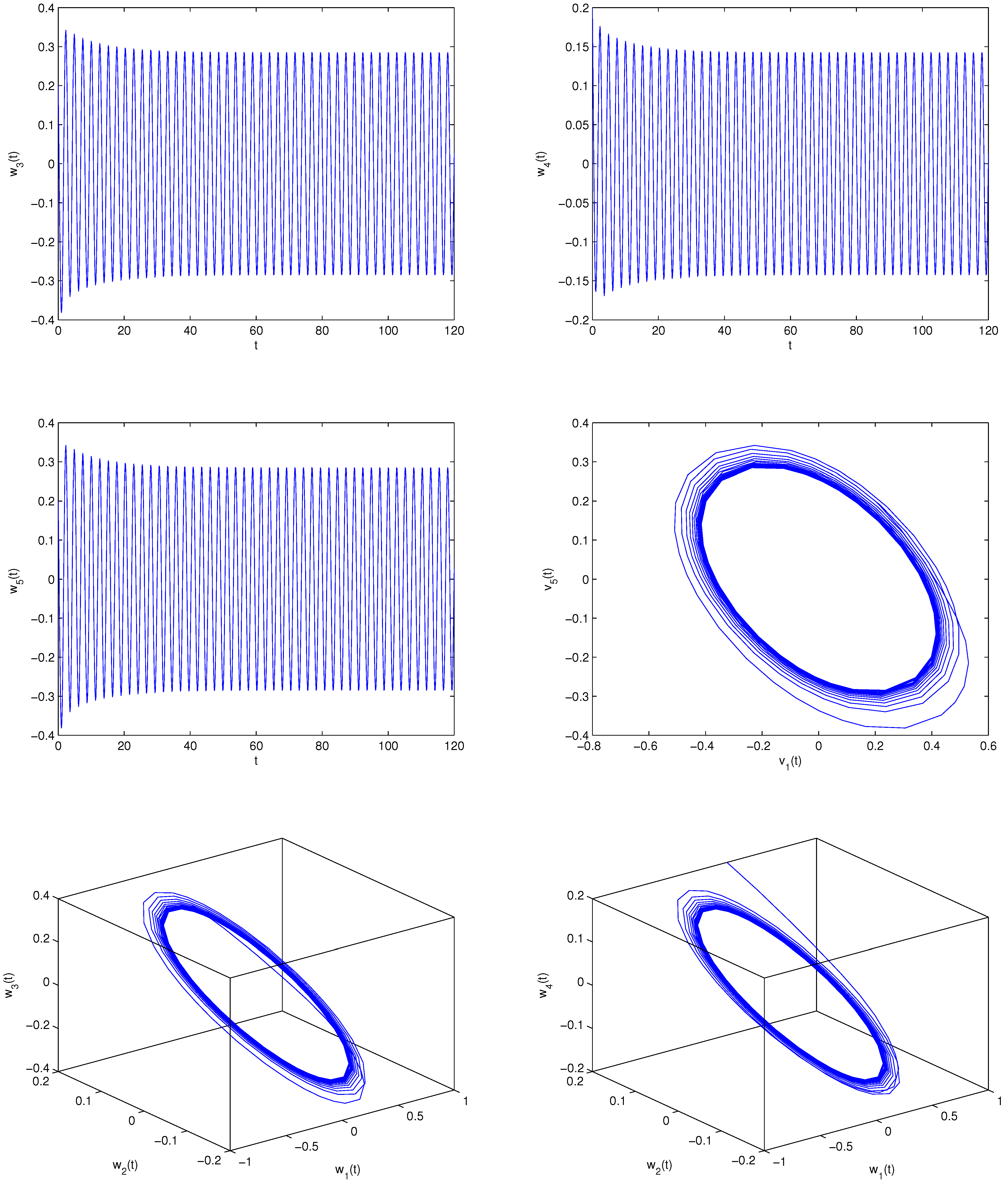
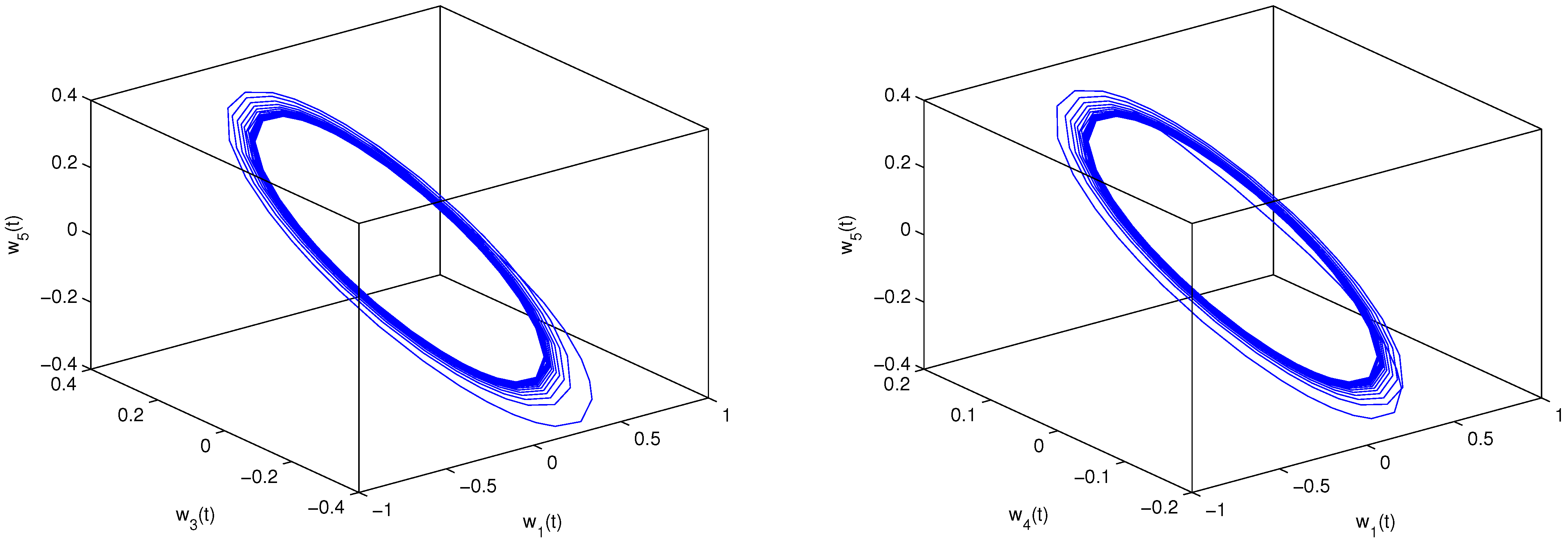
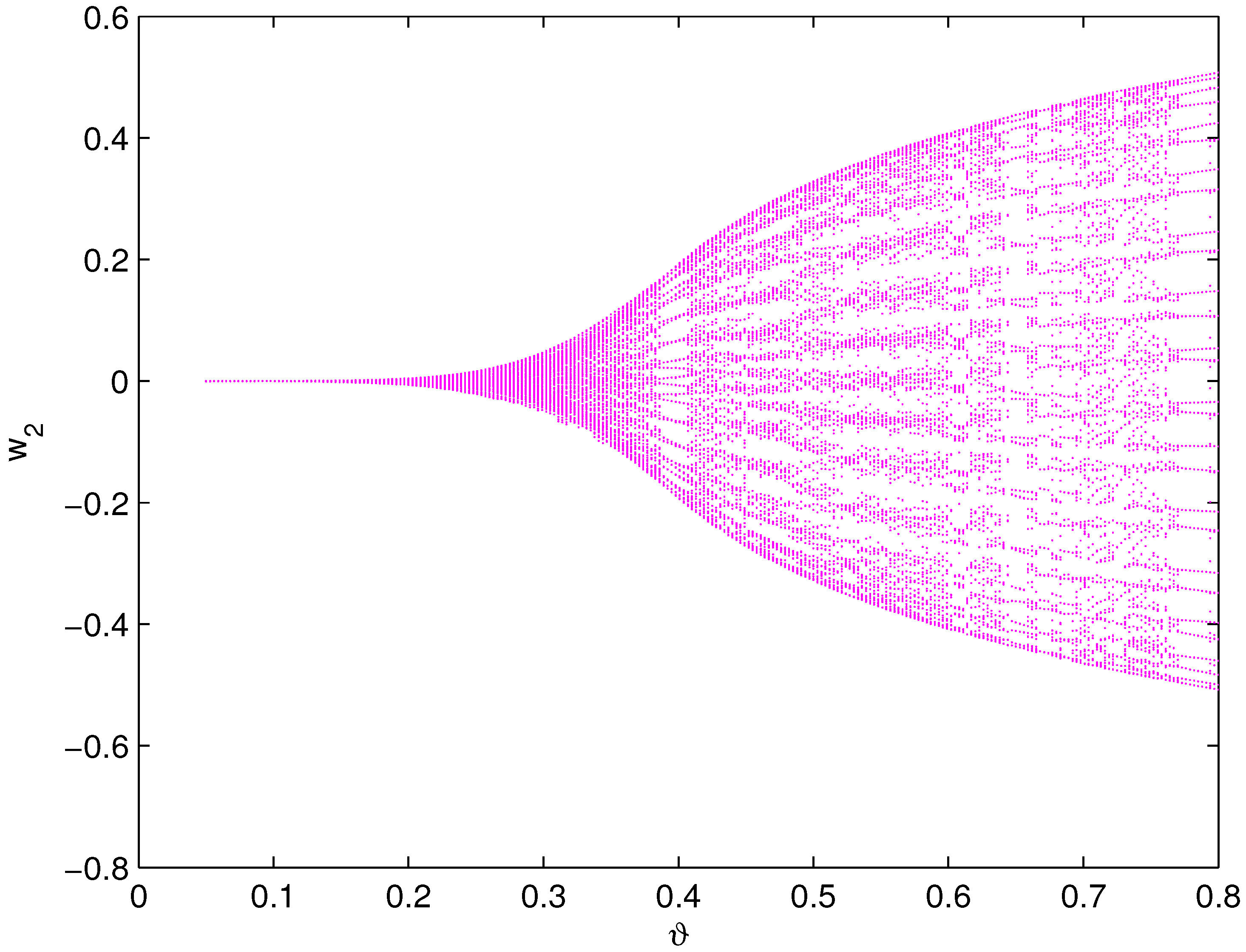
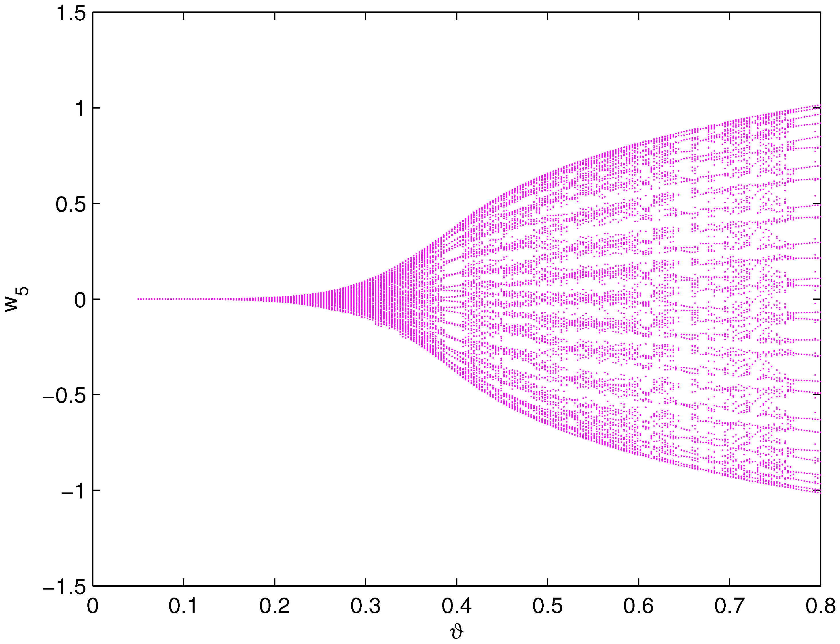
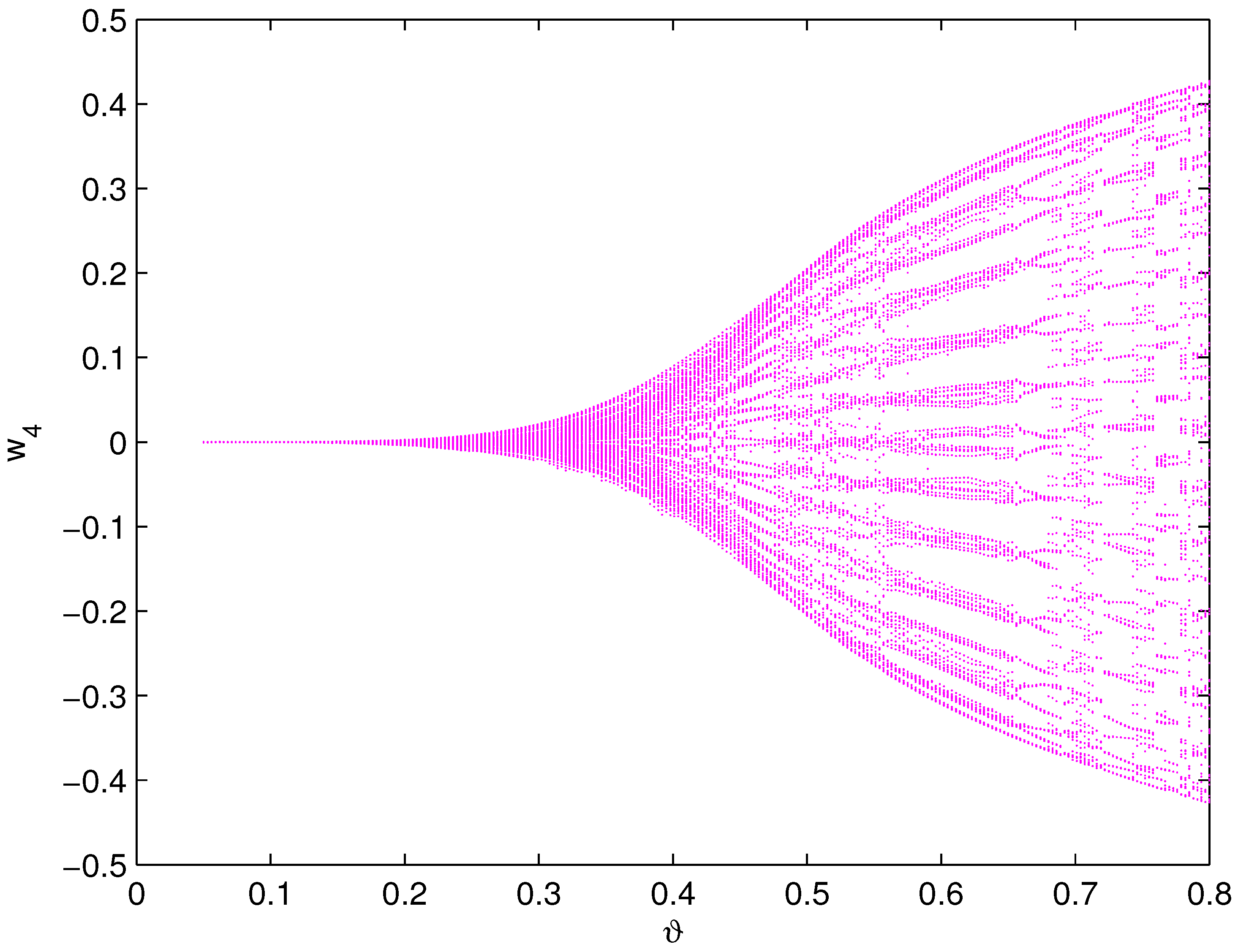
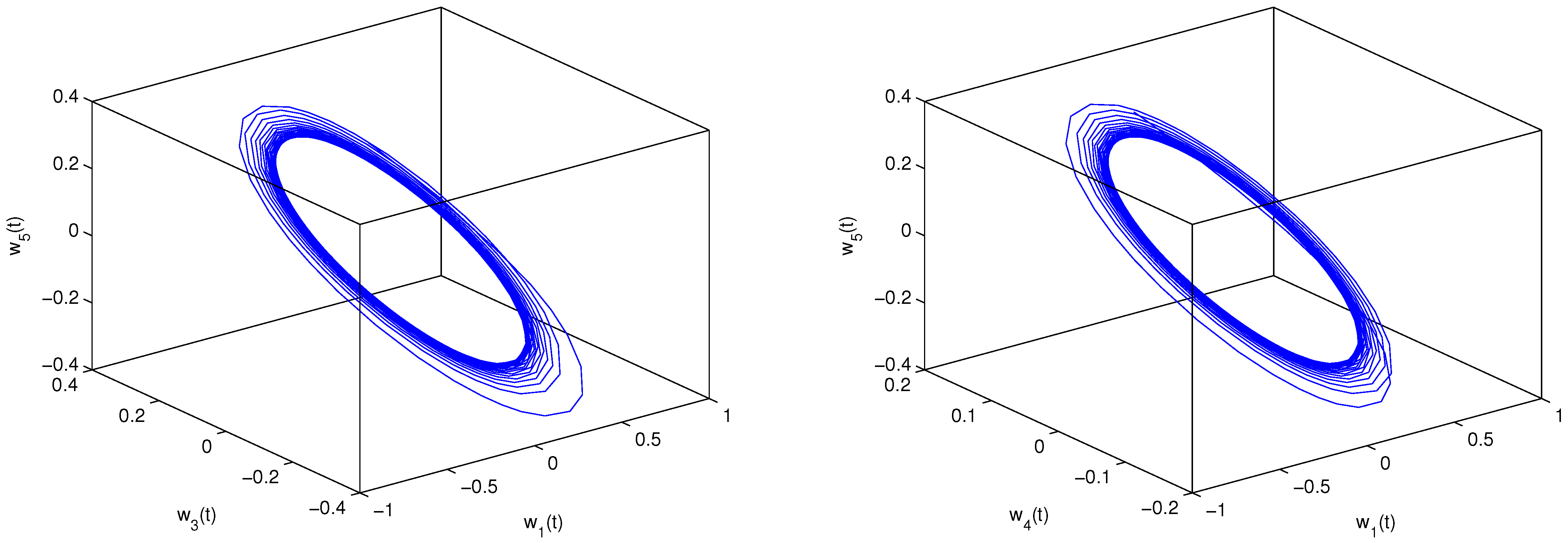
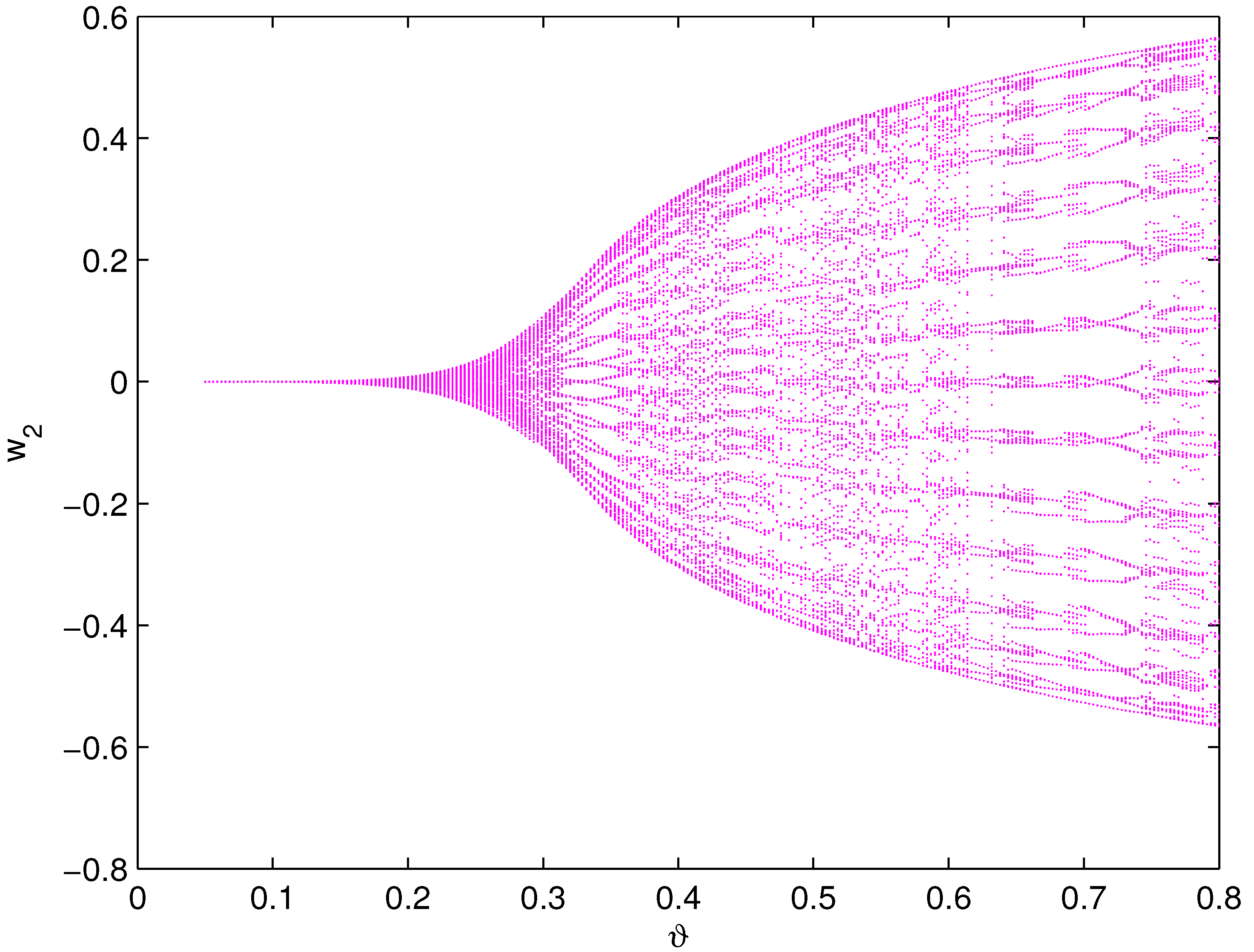
7. Computer Simulations

Example 1.

We begin with the following fractional delayed BAM neural network models:

$$\left\{\begin{array}{c}{\displaystyle \frac{d^{0.92}{y}_1\left(t\right)}{d{t}^{0.92}}=-1.3y_1\left(t\right)+2tanh\left(y_2(t-{\vartheta }_2)\right)+0.8tanh\left(y_3(t-{\vartheta }_2)\right)}\hfill \\ {\displaystyle 1.9tanh\left(y_4(t-{\vartheta }_2)\right)+1.3tanh\left(y_5(t-{\vartheta }_2)\right),}\hfill \\ {\displaystyle \frac{d^{0.92}{y}_2\left(t\right)}{d{t}^{0.92}}=-1.3y_2\left(t\right)-tanh\left(y_1(t-{\vartheta }_1)\right),}\hfill \\ {\displaystyle \frac{d^{0.92}{y}_3\left(t\right)}{d{t}^{0.92}}=-1.3y_3\left(t\right)-2tanh\left(y_1(t-{\vartheta }_1)\right),}\hfill \\ {\displaystyle \frac{d^{0.92}{y}_4\left(t\right)}{d{t}^{0.92}}=-1.3y_4\left(t\right)-tanh\left(y_1(t-{\vartheta }_1)\right),}\hfill \\ {\displaystyle \frac{d^{0.92}{y}_5\left(t\right)}{d{t}^{0.92}}=-1.3y_5\left(t\right)-2tanh\left(y_1(t-{\vartheta }_1)\right).}\hfill \end{array}\right.$$

(69)

Let

$$\left\{\begin{array}{c}{\displaystyle w_1\left(t\right)=y_1(t-{\vartheta }_1),}\hfill \\ {\displaystyle w_2\left(t\right)=y_2\left(t\right),}\hfill \\ {\displaystyle w_3\left(t\right)=y_3\left(t\right),}\hfill \\ {\displaystyle w_4\left(t\right)=y_4\left(t\right),}\hfill \\ {\displaystyle w_5\left(t\right)=y_5\left(t\right).}\hfill \end{array}\right.$$

(70)

Applying (70) and in view of $\left({\mathcal{A}}_4\right)$, we gain

$$\left\{\begin{array}{c}{\displaystyle \frac{d^{0.92}{w}_1\left(t\right)}{d{t}^{0.92}}=-1.3w_1\left(t\right)+2tanh\left(w_2(t-\vartheta )\right)+0.8tanh\left(w_3(t-\vartheta )\right)}\hfill \\ {\displaystyle +1.9tanh\left(w_4(t-\vartheta )\right)+1.3tanh\left(w_5(t-\vartheta )\right),}\hfill \\ {\displaystyle \frac{d^{0.92}{w}_2\left(t\right)}{d{t}^{0.92}}=-1.3w_2\left(t\right)-tanh\left(w_1\left(t\right)\right),}\hfill \\ {\displaystyle \frac{d^{0.92}{w}_3\left(t\right)}{d{t}^{0.92}}=-1.3w_3\left(t\right)-2tanh\left(w_1\left(t\right)\right),}\hfill \\ {\displaystyle \frac{d^{0.92}{w}_4\left(t\right)}{d{t}^{0.92}}=-1.3w_4\left(t\right)-tanh\left(w_1\left(t\right)\right),}\hfill \\ {\displaystyle \frac{d^{0.92}{w}_5\left(t\right)}{d{t}^{0.92}}=-1.3w_5\left(t\right)-2tanh\left(w_1\left(t\right)\right).}\hfill \end{array}\right.$$

(71)

Obviously, system (71) admits a unique null equilibrium point $E(0,0,0,0,0)$. Using Matlab software, we gain ${\vartheta }_0=0.37$. We can verify that $\left({\mathcal{A}}_1\right)$–$\left({\mathcal{A}}_6\right)$ of Theorem 3 are satisfied. Thus, if $\vartheta \in [0,0.37)$, the null equilibrium point $E(0,0,0,0,0)$ of system (71) remains locally asymptotically stable. For this case, we choose $\vartheta =0.35<{\vartheta }_0=0.37$; the Matlab simulation graphs are presented in Figure 1. Figure 1 shows the local asymptotic stability of the null equilibrium point $E(0,0,0,0,0)$ of system (71), i.e., every state of the neurons of neural network models (71) is close to null as $t\to +\infty .$ If $\vartheta \in [0.37,+\infty )$, then system (71) becomes unstable and a Hopf bifurcation arises. For this case, we choose $\vartheta =0.4>{\vartheta }_0=0.37$. The Matlab simulation plots are listed in Figure 2. Figure 2 confirms the onset of Hopf bifurcation around the null equilibrium point $E(0,0,0,0,0)$ of system (71), i.e., all the states of the neurons of neural networks (71) maintain periodic oscillatory level around the null equilibrium point $E(0,0,0,0,0)$. In order to display this nature intuitively, we provide the relevant bifurcation figures (see Figure 3, Figure 4, Figure 5, Figure 6 and Figure 7). Figure 3, Figure 4, Figure 5, Figure 6 and Figure 7 reveal the relation ϑ-$w_1$, ϑ-$w_2$, ϑ-$w_3$, ϑ-$w_4$, ϑ-$w_5$, respectively. From Figure 3, Figure 4, Figure 5, Figure 6 and Figure 7, we can see that the bifurcation number of system (71) is $0.37$.

Example 2.

Now, we take the following fractional controlled BAM neural network models:

$$\left\{\begin{array}{c}{\displaystyle \frac{d^{0.92}{w}_1\left(t\right)}{d{t}^{0.92}}=-1.3w_1\left(t\right)+2tanh\left(w_2(t-\vartheta )\right)+0.8tanh\left(w_3(t-\vartheta )\right)}\hfill \\ {\displaystyle +1.9tanh\left(w_4(t-\vartheta )\right)+1.3tanh\left(w_5(t-\vartheta )\right)+\gamma [w_1(t-\vartheta )-w_1\left(t\right)],}\hfill \\ {\displaystyle \frac{d^{0.92}{w}_2\left(t\right)}{d{t}^{0.92}}=-1.3w_2\left(t\right)-tanh\left(w_1\left(t\right)\right),}\hfill \\ {\displaystyle \frac{d^{0.92}{w}_3\left(t\right)}{d{t}^{0.92}}=-1.3w_3\left(t\right)-2tanh\left(w_1\left(t\right)\right),}\hfill \\ {\displaystyle \frac{d^{0.92}{w}_4\left(t\right)}{d{t}^{0.92}}=-1.3w_4\left(t\right)-tanh\left(w_1\left(t\right)\right),}\hfill \\ {\displaystyle \frac{d^{0.92}{w}_5\left(t\right)}{d{t}^{0.92}}=-1.3w_5\left(t\right)-2tanh\left(w_1\left(t\right)\right).}\hfill \end{array}\right.$$

(72)

Obviously, system (72) admits a unique null equilibrium point $E(0,0,0,0,0)$. Let $\gamma =0.5$. Using Matlab software, we gain ${\vartheta }_{*}=0.44$. We can verify that $\left({\mathcal{A}}_1\right),\left({\mathcal{A}}_2\right),\left({\mathcal{A}}_3\right),\left({\mathcal{A}}_4\right),\left({\mathcal{A}}_7\right),\left({\mathcal{A}}_8\right)$ of Theorem 4 are satisfied. Thus, if $\vartheta \in [0,0.44)$, then the null equilibrium point $E(0,0,0,0,0)$ of system (72) retains local asymptotic stability. For this case, we choose $\vartheta =0.42<{\vartheta }_{*}=0.44$; the Matlab simulation graphs are presented in Figure 8. Figure 8 shows the local asymptotic stability of the null equilibrium point $E(0,0,0,0,0)$ of system (72), i.e., every state of the neurons of neural network models (72) are as close to null as $t\to +\infty .$ If $\vartheta \in [0.44,+\infty )$, then system (72) becomes unstable and a Hopf bifurcation arises. For this case, we choose $\vartheta =0.5>{\vartheta }_{*}=0.44$. The Matlab simulation graphs are listed in Figure 9. Figure 9 confirms the onset of Hopf bifurcation around the null equilibrium point $E(0,0,0,0,0)$ of system (72), i.e., every state of the neurons of neural networks (72) maintains a periodic oscillatory level around the null equilibrium point $E(0,0,0,0,0)$. In order to display this nature more intuitively, we provide the relevant bifurcation figures (see Figure 10, Figure 11, Figure 12, Figure 13 and Figure 14). Figure 10, Figure 11, Figure 12, Figure 13 and Figure 14 reveal the relation of ϑ-$w_1$, ϑ-$w_2$, ϑ-$w_3$, ϑ-$w_4$, ϑ-$w_5$, respectively. From Figure 10, Figure 11, Figure 12, Figure 13 and Figure 14, it can be seen that the bifurcation number of system (72) is $0.44$.

Example 3.

In this example, we have the following fractional controlled BAM neural network models:

$$\left\{\begin{array}{c}{\displaystyle \frac{d^{0.92}{w}_1\left(t\right)}{d{t}^{0.92}}=-1.3w_1\left(t\right)+2tanh\left(w_2(t-\vartheta )\right)+0.8tanh\left(w_3(t-\vartheta )\right)}\hfill \\ {\displaystyle +1.9tanh\left(w_4(t-\vartheta )\right)+1.3tanh\left(w_5(t-\vartheta )\right)+\gamma [w_1(t-\vartheta )-w_1\left(t\right)],}\hfill \\ {\displaystyle \frac{d^{0.92}{w}_2\left(t\right)}{d{t}^{0.92}}=-1.3w_2\left(t\right)-tanh\left(w_1\left(t\right)\right),}\hfill \\ {\displaystyle \frac{d^{0.92}{w}_3\left(t\right)}{d{t}^{0.92}}=-1.3w_3\left(t\right)-2tanh\left(w_1\left(t\right)\right),}\hfill \\ {\displaystyle \frac{d^{0.92}{w}_4\left(t\right)}{d{t}^{0.92}}=-1.3w_4\left(t\right)-tanh\left(w_1\left(t\right)\right),}\hfill \\ {\displaystyle \frac{d^{0.92}{w}_5\left(t\right)}{d{t}^{0.92}}=-1.3w_5\left(t\right)-2tanh\left(w_1\left(t\right)\right).}\hfill \end{array}\right.$$

(73)

Obviously, system (73) admits a unique null equilibrium point $E(0,0,0,0,0)$. Let $\gamma =-0.5$. Using Matlab software, we gain ${\vartheta }_{*}=0.32$. We can verify that $\left({\mathcal{A}}_1\right),\left({\mathcal{A}}_2\right),\left({\mathcal{A}}_3\right),\left({\mathcal{A}}_4\right),\left({\mathcal{A}}_7\right),\left({\mathcal{A}}_8\right)$ of Theorem 4 are satisfied. Thus, if $\vartheta \in [0,0.32)$, then the null equilibrium point $E(0,0,0,0,0)$ of system (73) is locally asymptotically stable. For this case, we choose $\vartheta =0.3<{\vartheta }_{*}=0.32$; the Matlab simulation graphs are presented in Figure 15. Figure 15 shows the local asymptotic stability of the null equilibrium point $E(0,0,0,0,0)$ of system (73), i.e., all the states of the neurons of neural networks (73) are close to zero as $t\to +\infty .$ If $\vartheta \in [0.32,+\infty )$, then system (73) becomes unstable and a Hopf bifurcation arises. For this case, we choose $\vartheta =0.33>{\vartheta }_{*}=0.32$. The Matlab simulation graphs are listed in Figure 16. Figure 16 confirms the onset of Hopf bifurcation around the null equilibrium point $E(0,0,0,0,0)$ of system (73), i.e., every state of the neurons of neural network models (73) maintains a periodic oscillatory level around the null equilibrium point $E(0,0,0,0,0)$. In order to display this property intuitively, we provide the relevant bifurcation figures (see Figure 17, Figure 18, Figure 19, Figure 20 and Figure 21). Figure 17, Figure 18, Figure 19, Figure 20 and Figure 21 reveal the relation of ϑ-$w_1$, ϑ-$w_2$, ϑ-$w_3$, ϑ-$w_4$, ϑ-$w_5$, respectively. From Figure 17, Figure 18, Figure 19, Figure 20 and Figure 21, it can easily be seen that the bifurcation number of system (73) is $0.32$.

Remark 2.

Relying on the numerical simulation results for Examples 1–Example 3, we know that the bifurcation number of system (71) is $0.37$, the bifurcation value of system (72) is $0.44$, and the bifurcation number of system (73) is $0.33$. Thus, we can conclude that it is possible to effectively enlarge (reduce) the stability region and delay (shorten) the time of onset of Hopf bifurcation for system (71) by adjusting the feedback gain coefficient.

8. Conclusions

During the past several decades, neural networks have attracted great interest because of their wide application in various areas. Relying on earlier publications, we have proposed a class of new fractional-order BAM neural networks concerning five neurons and delays and systematically analyzed the existence, uniqueness, and boundedness of the solution of the involved fractional-order BAM neural networks. Moreover, we acquire a new delay-independent condition of the stability and bifurcation of the involved fractional-order BAM neural networks. Making use of a speed feedback controller, we successfully control the stability domain and time of Hopf bifurcation of the involved fractional-order BAM neural networks. The results obtained from this study have important theoretical significance in dominating neural networks. There are other control techniques that can be applied to control the Hopf bifurcation of fractional-order BAM neural networks. For example, the Hopf bifurcation of fractional-order BAM neural networks we can be controlled by a delayed feedback controller, hybrid controller, $P{D}^p$ controller, etc. We leave these as future research directions.

References

1. Wang, P.; Li, X.C.; Wang, N.; Li, Y.Y.; Shi, K.B.; Lu, J.Q. Almost periodic synchronization of quaternion-valued fuzzy cellular neural networks with leakage delays. Fuzzy Sets Syst. 2022, 426, 46–65. [Google Scholar] [CrossRef]
2. Aouiti1, C.; M’hamdi, M.S.; Touati, A. Pseudo almost automorphic solution of recurrent neural networks with time-varying coefficients and mixed delays. Neural Process. Lett. 2017, 45, 121–140. [Google Scholar] [CrossRef]
3. Xu, C.J.; Li, P.L.; Pang, Y.C. Exponential stability of almost periodic solutions for memristor-based neural networks with distributed leakage delays. Neural Comput. 2016, 28, 2726–2756. [Google Scholar] [CrossRef] [PubMed]
4. Xu, C.J.; Zhang, Q.M. On anti-periodic solutions for Cohen-Grossberg shunting inhibitory neural networks with time-varying delays and impulses. Neural Comput. 2014, 26, 2328–2349. [Google Scholar] [CrossRef] [PubMed]
5. Karnan, A.; Nagamani, G. Non-fragile state estimation for memristive cellular neural networks with proportional delay. Math. Comput. Simul. 2022, 193, 217–231. [Google Scholar] [CrossRef]
6. Li, Y.K.; Shen, S.P. Almost automorphic solutions for Clifford-valued neutral-type fuzzy cellular neural networks with leakage delays on time scales. Neurocomputing 2020, 417, 23–35. [Google Scholar] [CrossRef]
7. Xu, C.J.; Liao, M.X.; Li, P.L.; Liu, Z.X.; Yuan, S. New results on pseudo almost periodic solutions of quaternion-valued fuzzy cellular neural networks with delays. Fuzzy Sets Syst. 2021, 411, 25–47. [Google Scholar] [CrossRef]
8. Cui, W.X.; Wang, Z.J.; Jin, W.B. Fixed-time synchronization of Markovian jump fuzzy cellular neural networks with stochastic disturbance and time-varying delays. Fuzzy Sets Syst. 2021, 411, 68–84. [Google Scholar] [CrossRef]
9. Huang, C.X.; Wen, S.G.; Huang, L.H. Dynamics of anti-periodic solutions on shunting inhibitory cellular neural networks with multi-proportional delays. Neurocomputing 2019, 357, 47–52. [Google Scholar] [CrossRef]
10. Ali, M.S.; Yogambigai, J.; Saravanan, S.; Elakkia, S. Stochastic stability of neutral-type Markovian-jumping BAM neural networks with time varying delays. J. Comput. Appl. Math. 2019, 349, 142–156. [Google Scholar] [CrossRef]
11. Sowmiya, C.; Raja, R.; Zhu, Q.X.; Rajchakit, G. Further mean-square asymptotic stability of impulsive discrete-time stochastic BAM neural networks with Markovian jumping and multiple time-varying delays. J. Frankl. Inst. 2019, 356, 561–591. [Google Scholar] [CrossRef]
12. Oliveira, J.J. Global stability criteria for nonlinear differential systems with infinite delay and applications to BAM neural networks. Chaos Solitons Fractals 2022, 164, 112676. [Google Scholar] [CrossRef]
13. Zhang, T.W.; Li, Y.K. Global exponential stability of discrete-time almost automorphic Caputo-Fabrizio BAM fuzzy neural networks via exponential Euler technique. Knowl.-Based Syst. 2022, 246, 108675. [Google Scholar] [CrossRef]
14. Thoiyab, N.M.; Muruganantham, P.; Zhu, Q.X.; Gunasekaran, N. Novel results on global stability analysis for multiple time-delayed BAM neural networks under parameter uncertainties. Chaos Solitons Fractals 2021, 152, 111441. [Google Scholar] [CrossRef]
15. Xu, C.J.; Liao, M.X.; Li, P.L.; Guo, Y.; Liu, Z.X. Bifurcation properties for fractional order delayed BAM neural networks. Cogn. Comput. 2021, 13, 322–356. [Google Scholar] [CrossRef]
16. Du, W.T.; Xiao, M.; Ding, J.; Yao, Y.; Wang, Z.X.; Yang, X.S. Fractional-order PD control at Hopf bifurcation in a delayed predator-prey system with trans-species infectious diseases. Math. Comput. Simul. 2023, 205, 414–438. [Google Scholar] [CrossRef]
17. Xu, C.J.; Zhang, W.; Liu, Z.X.; Yao, L.Y. Delay-induced periodic oscillation for fractional-order neural networks with mixed delays. Neurocomputing 2022, 488, 681–693. [Google Scholar] [CrossRef]
18. Xu, C.J.; Liu, Z.X.; Liao, M.X.; Yao, L.Y. Theoretical analysis and computer simulations of a fractional order bank data model incorporating two unequal time delays. Expert Syst. Appl. 2022, 199, 116859. [Google Scholar] [CrossRef]
19. Xu, C.J.; Mu, D.; Liu, Z.X.; Pang, Y.C.; Liao, M.X.; Yao, P.L.L.L.Y.; Qin, Q.W. Comparative exploration on bifurcation behavior for integer-order and fractional-order delayed BAM neural networks. Nonlinear Anal. Model. Control 2022. [Google Scholar] [CrossRef]
20. Huang, C.D.; Wang, J.; Chen, X.P.; Cao, J.D. Bifurcations in a fractional-order BAM neural network with four different delays. Neural Netw. 2021, 141, 344–354. [Google Scholar] [CrossRef]
21. Bentout, S.; Djilali, S.; Kumar, S. Mathematical analysis of the influence of prey escaping from prey herd on three species fractional predator-prey interaction model. Phys. A Stat. Mech. Appl. 2021, 572, 125840. [Google Scholar] [CrossRef]
22. Deshpande, A.S.; Daftardar-Gejji, V.; Sukale, Y.V. On Hopf bifurcation in fractional dynamical systems. Chaos Solitons Fractals 2017, 98, 189–198. [Google Scholar] [CrossRef]
23. Vivek, D.; Kanagarajan, K.; Elsayed, E.M. Some existence and stability results for Hilfer-fractional implicit differential equations with nonlocal conditions. Mediterr. J. Math. 2018, 15, 1–21. [Google Scholar] [CrossRef]
24. Harikrishnan, S.; Kanagarajan, K.; Elsayed, E.M. Existence and stability results for differential equations with complex order involving Hilfer fractional derivative. TWMS J. Pure Appl. Math. 2019, 10, 94–101. [Google Scholar]
25. Ci, J.X.; Guo, Z.Y.; Long, H.; Wen, S.P.; Huang, T.W. Multiple asymptotical ω-periodicity of fractional-order delayed neural networks under state-dependent switching. Neural Netw. 2023, 157, 11–25. [Google Scholar] [CrossRef]
26. Lin, Y.T.; Wang, J.L.; Liu, C.G. Output synchronization analysis and PD control for coupled fractional-order neural networks with multiple weights. Neurocomputing 2023, 519, 17–25. [Google Scholar] [CrossRef]
27. Xiao, J.; Wu, L.; Wu, A.L.; Zeng, Z.G.; Zhang, Z. Novel controller design for finite-time synchronization of fractional-order memristive neural networks. Neurocomputing 2022, 512, 494–502. [Google Scholar] [CrossRef]
28. Zhang, X.L.; Li, H.L.; Kao, Y.G.; Zhang, L.; Jiang, H.J. Global Mittag-Leffler synchronization of discrete-time fractional-order neural networks with time delays. Appl. Math. Comput. 2022, 433, 127417. [Google Scholar] [CrossRef]
29. Qiu, H.L.; Cao, J.D.; Liu, H. Passivity of fractional-order coupled neural networks with interval uncertainties. Math. Comput. Simul. 2023, 205, 845–860. [Google Scholar] [CrossRef]
30. Ali, M.S.; Narayanan, G.; Sevgen, S.; Shekher, V.; Arik, S. Global stability analysis of fractional-order fuzzy BAM neural networks with time delay and impulsive effects. Commun. Nonlinear Sci. Numer. Simul. 2019, 78, 104853. [Google Scholar]
31. Popa, C.A. Mittag–CLeffler stability and synchronization of neutral-type fractional-order neural networks with leakage delay and mixed delays. J. Frankl. Inst. 2022. [Google Scholar] [CrossRef]
32. Shafiya, M.; Nagamani, G. New finite-time passivity criteria for delayed fractional-order neural networks based on Lyapunov function approach. Chaos Solitons Fractals 2022, 158, 112005. [Google Scholar] [CrossRef]
33. Huang, C.D.; Nie, X.B.; Zhao, X.; Song, Q.K.; Tu, Z.W.; Xiao, M.; Cao, J.D. Novel bifurcation results for a delayed fractional-order quaternion-valued neural network. Neural Netw. 2019, 117, 67–93. [Google Scholar] [CrossRef] [PubMed]
34. Xu, C.J.; Mu, D.; Pan, Y.L.; Aouiti, C.; Pang, Y.C.; Yao, L.Y. Probing into bifurcation for fractional-order BAM neural networks concerning multiple time delays. J. Comput. Sci. 2022, 62, 101701. [Google Scholar] [CrossRef]
35. Huang, C.D.; Meng, Y.J.; Cao, J.D.; Alsaedi, A.; Alsaadi, F.E. New bifurcation results for fractional BAM neural network with leakage delay. Chaos Solitons Fractals 2017, 100, 31–44. [Google Scholar] [CrossRef]
36. Kaslik, E.; Rădulescu, I.R. Stability and bifurcations in fractional-order gene regulatory networks. Appl. Math. Comput. 2022, 421, 126916. [Google Scholar] [CrossRef]
37. Xu, C.J.; Liu, Z.X.; Aouiti, C.; Li, P.L.; Yao, L.Y.; Yan, J.L. New exploration on bifurcation for fractional-order quaternion-valued neural networks involving leakage delays. Cogn. Neurodyn. 2022, 16, 1233–1248. [Google Scholar] [CrossRef]
38. Wang, Y.L.; Cao, J.D.; Huang, C.D. Exploration of bifurcation for a fractional-order BAM neural network with n+2 neurons and mixed time delays. Chaos Solitons Fractals 2022, 159, 112117. [Google Scholar] [CrossRef]
39. Li, S.; Huang, C.D.; Yuan, S.L. Hopf bifurcation of a fractional-order double-ring structured neural network model with multiple communication delays. Nonlinear Dyn. 2022, 108, 379–396. [Google Scholar] [CrossRef]
40. Mo, S.S.; Huang, C.D.; Cao, J.D.; Alsaedi, A. Dynamical bifurcations in a fractional-order neural network with nonidentical communication delays. Cogn. Comput. 2022. [Google Scholar] [CrossRef]
41. Yang, Y.; Ye, J. Stability and bifurcation in a simplified five-neuron BAM neural networks with delays. Chaos Solitons Fractals 2009, 42, 2357–2363. [Google Scholar] [CrossRef]
42. Podlubny, I. Fractional Differential Equations; Academic Press: New York, NY, USA, 1999. [Google Scholar]
43. Bandyopadhyay, B.; Kamal, S. Stabliization and Control of Fractional Order Systems: A Sliding Mode Approach; Springer: Heidelberg, Germany, 2015; Volume 317. [Google Scholar]
44. Li, Y.; Chen, Y.Q.; Podlubny, I. Stability of fractional-order nonlinear dynamic systems: Lyapunov direct method and generalized Mittag-Leffler stability. Comput. Math. Appl. 2009, 59, 1810–1821. [Google Scholar] [CrossRef] [Green Version]
45. Li, H.L.; Zhang, L.; Hu, C.; Jiang, Y.L.; Teng, Z.D. Dynamical analysis of a fractional-order predator-prey model incorporating a prey refuge. J. Appl. Math. Comput. 2017, 54, 435–449. [Google Scholar] [CrossRef]
46. Matignon, D. Stability results for fractional differential equations with applications to control processing. Comput. Eng. Syst. Appl. 1996, 2, 963–968. [Google Scholar]
47. Wang, X.H.; Wang, Z.; Xia, J.W. Stability and bifurcation control of a delayed fractional-order eco-epidemiological model with incommensurate orders. J. Frankl. Inst. 2019, 356, 8278–8295. [Google Scholar] [CrossRef]
48. Deng, W.H.; Li, C.P.; Lü, J.H. Stability analysis of linear fractional differential system with multiple time delays. Nonlinear Dyn. 2007, 48, 409–416. [Google Scholar] [CrossRef]
49. Yu, P.; Chen, G.R. Hopf bifurcation control using nonlinear feedback with polynomial functions. Int. J. Bifurc. Chaos 2004, 14, 1683–1704. [Google Scholar] [CrossRef]
Figure 1. Matlab simulation outcomes for system (71) when ϑ = 0.35 < ϑ 0 = 0.37 . The null equilibrium point E ( 0 , 0 , 0 , 0 , 0 ) of system (71) keeps locally asymptotic stability.
Fractalfract 07 00007 g001aFractalfract 07 00007 g001b
Figure 2. Matlab simulation outcomes for system (71) when ϑ = 0.4 > ϑ 0 = 0.37 . System (71) generates a Hopf bifurcation near the null equilibrium point E ( 0 , 0 , 0 , 0 , 0 ) .
Fractalfract 07 00007 g002aFractalfract 07 00007 g002bFractalfract 07 00007 g002c
Figure 3. Bifurcation graph of system (71): the time delay ϑ versus the variable w 1 . The bifurcation number is 0.37 .
Fractalfract 07 00007 g003
Figure 4. Bifurcation graph of system (71): the delay ϑ versus the variable w 2 . The bifurcation number is 0.37 .
Fractalfract 07 00007 g004
Figure 5. Bifurcation graph of system (71): the delay ϑ versus the variable w 3 . The bifurcation number is 0.37 .
Fractalfract 07 00007 g005
Figure 6. Bifurcation graph of system (71): the delay ϑ versus the variable w 4 . The bifurcation number is 0.37 .
Fractalfract 07 00007 g006
Figure 7. Bifurcation graph of system (71): the delay ϑ versus the variable w 5 . The bifurcation number is 0.37 .
Fractalfract 07 00007 g007
Figure 8. Matlab simulation results for system (72) when ϑ = 0.42 < ϑ * = 0.44 . The null equilibrium point E ( 0 , 0 , 0 , 0 , 0 ) of system (72) keeps locally asymptotic stability.
Fractalfract 07 00007 g008aFractalfract 07 00007 g008b
Figure 9. Matlab simulation outcomes for system (72) when ϑ = 0.5 > ϑ * = 0.44 . System (70) generates a Hopf bifurcation near the null equilibrium point E ( 0 , 0 , 0 , 0 , 0 ) .
Fractalfract 07 00007 g009aFractalfract 07 00007 g009bFractalfract 07 00007 g009c
Figure 10. Bifurcation graph of system (72): the time delay ϑ versus the variable w 1 . The bifurcation number is 0.44 .
Fractalfract 07 00007 g010
Figure 11. Bifurcation graph of system (72): the time delay ϑ versus the variable w 2 . The bifurcation number is 0.44 .
Fractalfract 07 00007 g011
Figure 12. Bifurcation graph of system (72): the delay ϑ versus the variable w 3 . The bifurcation number is 0.44 .
Fractalfract 07 00007 g012
Figure 13. Bifurcation graph of system (72): the delay ϑ versus the variable w 4 . The bifurcation number is 0.44 .
Fractalfract 07 00007 g013
Figure 14. Bifurcation graph of system (72): the time delay ϑ versus the variable w 5 . The bifurcation number is 0.44 .
Fractalfract 07 00007 g014
Figure 15. Matlab simulation outcomes for system (73) when ϑ = 0.3 < ϑ * = 0.32 . The null equilibrium point E ( 0 , 0 , 0 , 0 , 0 ) of system (73) keeps locally asymptotic stability.
Fractalfract 07 00007 g015aFractalfract 07 00007 g015b
Figure 16. Matlab simulation outcomes for system (73) when ϑ = 0.33 > ϑ * = 0.32 . System (73) generates a Hopf bifurcation near the null equilibrium point E ( 0 , 0 , 0 , 0 , 0 ) .
Fractalfract 07 00007 g016aFractalfract 07 00007 g016bFractalfract 07 00007 g016c
Figure 17. Bifurcation graph of system (73): the time delay ϑ versus the variable w 1 . The bifurcation number is 0.32 .
Fractalfract 07 00007 g017
Figure 18. Bifurcation graph of system (73): the time delay ϑ versus the variable w 2 . The bifurcation number is 0.32 .
Fractalfract 07 00007 g018
Figure 19. Bifurcation graph of system (73): the time delay ϑ versus the variable w 3 . The bifurcation number is 0.32 .
Fractalfract 07 00007 g019
Figure 20. Bifurcation graph of system (73): the time delay ϑ versus the variable w 4 . The bifurcation number is 0.32 .
Fractalfract 07 00007 g020
Figure 21. Bifurcation graph of system (73): the time delay ϑ versus the variable w 5 . The bifurcation number is 0.32 .
Fractalfract 07 00007 g021
Disclaimer/Publisher’s Note: The statements, opinions and data contained in all publications are solely those of the individual author(s) and contributor(s) and not of MDPI and/or the editor(s). MDPI and/or the editor(s) disclaim responsibility for any injury to people or property resulting from any ideas, methods, instructions or products referred to in the content.