Fractional-Order Financial System and Fixed-Time Synchronization

Abstract

This study is concerned with the dynamic investigation and fixed-time synchronization of a fractional-order financial system with the Caputo derivative. The rich dynamic behaviors of the fractional-order financial system with variations of fractional orders and parameters are discussed analytically and numerically. Through using phase portraits, bifurcation diagrams, maximum Lyapunov exponent diagrams, 0–1 testing and time series, it is found that chaos exists in the proposed fractional-order financial system. Additionally, a complexity analysis is carried out utilizing approximation entropy SE and C₀ complexity to detect whether chaos exists. Furthermore, a synchronization controller and an adaptive parameter update law are designed to synchronize two fractional-order chaotic financial systems and identify the unknown parameters in fixed time simultaneously. The estimate of the setting time of synchronization depends on the parameters of the designed controller and adaptive parameter update law, rather than on the initial conditions. Numerical simulations show the effectiveness of the theoretical results obtained.

1. Introduction

Fractional-order calculus, a generalization of integer-order calculus, has an equally long history as integer-order calculus, but due to the limited computational power in the past, fractional-order calculus has not received much attention until recent decades when computational power improved. Fractional-order calculus can describe chaos and different nonlinear phenomena more accurately than integer-order derivatives. Recently, with the rapid progress of chaos theory and applied research, fractional-order chaotic systems [1,2,3,4,5,6,7,8,9] have received wide attention and undergone rapid development. Yuan et al. [2] studied chaos and the bifurcation of fractional semi-logistic maps based on the Lyapunov exponent, the Schwarzian derivative, Shannon entropy and Kolmogorov entropy. Chen et al. [3] proposed a three-dimensional fractional-order discrete Hopfield neural network; the dynamic behavior and synchronization were studied, and the system constructed was applied to image encryption. He et al. [4] investigated the dynamics and complexity of the fractional order digital manufacturing supply chain system; the nonlinear feedback controllers were designed to control and synchronize the chaos in the system. Mahmoud et al. [8] studied the dynamic analysis of a fractional chaotic ecological model, and the chaos control of the ecological model, using the adaptive sliding mode technique.

In the financial field, various economic problems are becoming increasingly complex due to the influence of nonlinear factors, and financial systems present extremely complex phenomena and characteristics. Therefore, it is necessary to investigate the dynamic characteristics and analyze chaotic effects of such complex financial systems in depth. In order to accurately grasp the operation laws of financial systems, researchers [10,11,12,13,14,15,16] have established various integer-order financial models to study the complex dynamic behaviors of the economy and society, revealing the intrinsic characteristics of economic development. However, studies have shown that economics and finance are extremely complex nonlinear systems involving many subjective factors, and there are many characteristics that cannot be described by the theory of integer calculus. Recently, the memory property of financial markets has attracted extensive interest, especially after Peters first proposed the Fractal Market Hypothesis (FMH) in [17]. The economic variables of financial systems are frequently affected by their historical information, and the concept of memory for economic processes has been discussed in [17,18,19]. It has been proven that fractional calculus has more obvious advantages in the memory and description of hereditary characteristics than integer calculus. So, the construction of financial systems is suited to fractional order description [20,21,22,23,24,25,26,27,28,29,30]. Xin et al. [20] introduced an investment incentive in a three-dimensional integer-order chaotic financial system and expanded it into a four-dimensional fractional-order chaotic financial system. Jahanshahi et al. [26] investigated hyperchaos and the predictive control of an economic system with variable-order fractional derivatives. Zhang et al. [27] studied the synchronization of fractal fractional-order hyperchaotic financial systems with model uncertainties and external perturbations. In Ref. [29], the authors analyzed a new financial chaotic model in fractional stochastic differential equations with the Atangana-Baleanu operator. The chaotic phenomenon makes prediction impossible in the financial world, and so it is very useful to avoid chaos in financial system.

On the other hand, many researchers [31,32,33,34,35,36,37,38,39] have shown great interest in the subjects of chaotic synchronization and control. Various control methods have been developed to regulate synchronization behavior, such as adaptive control [36], feedback control [37], impulsive control [38], intermittent control [39], and so on. It is more regrettable that all of the above techniques have only considered asymptotic stability. The asymptotic stability of synchronization can be achieved when time grows to infinity. We know that the convergence rate can effectively reflect the synchronization efficiency. Recently, finite-time stability was proposed in [40], which can allow finite-time convergence, called setting time. The finite-time synchronization of chaotic systems was studied in [41,42,43]. Although finite-time synchronization can achieve faster convergence, the setting time is affected by the initial conditions of the system, and there may be cases wherein the exact initial values are unknown; in addition, extreme initial values can lead to inaccurate estimates of the setting time. To overcome the drawbacks, fixed-time stability was proposed in [44], where the setting time does not depend on the initial conditions. The fixed-time stability of control systems has been a popular research topic in recent years [45,46,47,48,49,50]. However, there are countries around the world that wish to come out of the financial crisis in a short period of time. So, fixed-time synchronization and parameter identification are interesting in the financial field, particularly in the fractional-order chaotic financial system. This is the motivation for this paper.

Driven by the above discussions, in this paper, a fractional-order financial model is proposed by applying the Caputo fractional derivative operator to the integer case [29]. The dynamic behaviors of the fractional-order financial system are analyzed by bifurcation diagrams, maximum Lyapunov exponent diagrams, phase portraits, complexity diagrams and $p–s$ plots by $0–1$ testing. The results show that the fractional-order financial system has rich dynamics. Furthermore, the fixed-time synchronization and parameter identification problem of fractional-order chaotic financial systems are investigated by designing appropriate controllers and adaptive parameter update laws, in which synchronization can be achieved and parameters can be identified within the setting time regardless of the initial conditions. Finally, the effectiveness of the present theory is verified by numerical simulations. The contributions of this paper are summarized as follows:

• A financial model with a Caputo operator is constructed, which reflects the memory property of the financial system. The dynamic behaviors of the fractional-order financial system with variations of fractional orders and parameters are studied;
• The fixed-time synchronization and identification of the unknown parameters are realized. The resulting setting time of the fractional-order control system depends only on the parameters of the controller and the order of the fractional-order derivative;
• The proposed fixed-time synchronization method is applied to fractional-order chaotic financial systems, which has theoretical and practical significance.

The rest of this paper is organized as follows. Firstly, preliminaries and algorithms are given, and the model is established in Section 2. Then, in Section 3, the dynamic behaviors and the equilibrium points of the fractional-order financial system are discussed. Afterwards, in Section 4, a fixed-time synchronization controller and an adaptive parameter update law are designed. Lastly, the conclusion is presented in Section 5.

2. Preliminaries, Algorithms and Modeling

2.1. Preliminaries

There are many definitions of fractional order calculus [51,52], among which are the Grunwald–Letnikov (G-L) definition of fractional-order calculus, the Riemann–Liouville (R-L) definition of fractional-order calculus and the Caputo definition of fractional-order calculus. In this paper, the Caputo fractional derivative will be used.

Definition 1

[51,52]. The fractional integral of function $f(t)$ is

$${}_{t_0}{I}_t^{q}f(t)=\frac{1}{\Gamma (q)}{\displaystyle {\int }_{t_0}^t{(t-\tau )}^{q-1}f(\tau )d\tau },$$

(1)

where $t\ge t_0$ and $q>0$, and the gamma function is defined as

$$\Gamma (s)={\displaystyle {\int }_0^{\infty }{t}^{s-1}{e}^{-t}dt}.$$

(2)

Definition 2

[51,52]. The Caputo fractional derivative of function $f(t)$ of order$q$ is

$${}_{t_0}^C{D}_t^{q}f\left(t\right)=\frac{1}{\Gamma (n-q)}{\int }_{t_0}^t\frac{f^{\left(n\right)}\left(\tau \right)}{{(t-\tau )}^{q-n+1}}\mathrm{d}\tau ,$$

(3)

where $t\ge t_0$, and $n-1<q<n$ denotes a derivative order, in which $n\in N^{+}$.

Lemma 1

[51,52]. If the Caputo fractional derivative ${}_{t_0}{}^{C}D{}_t^{q}f(t)$ is integrable, then for$0<q\le 1$ and$t\in [t_0,\infty )$,${}_{t0}{I}_t^q{}_{t0}^C{D}_t^{q}f(t)=f(t)-f(t_0)$.

Lemma 2

[53]. Consider a fractional-order system as follows:

$$\frac{{\mathrm{d}}^{q}x(t)}{\mathrm{d}{t}^q}=f(x(t)),$$

(4)

where $x(0)={\left(x_1(0),x_2(0),\cdots ,x_n(0)\right)}^T\in {ℝ}^n$, $x(t)={\left(x_1(t),x_2(t),\dots ,x_n(t)\right)}^T\in {ℝ}^n$, $f:{\left[f_1,f_2,\dots ,f_n\right]}^T:{ℝ}^n\to {ℝ}^n$, and $q={(q_1,q_2,\cdots ,q_n)}^T$, $0<q_i<1(i=1,2,\cdots ,n)$. All equilibrium points of the system satisfy $f(x(t))=0$, so we substitute the above equilibrium points into the Jacobi matrix $J=\frac{\partial f}{\partial x}=\frac{\partial \left(f_1,f_2,\dots ,f_n\right)}{\partial \left(x_1,x_2,\dots ,x_n\right)}$; then, an equilibrium point is asymptotically stable if all eigenvalues ${\lambda }_i$ of $J$ satisfy $\left|\arg ({\lambda }_i)\right|>\frac{\pi q_m}{2}$, where $q_m=\max \left\{q_i\right\}$ and $i=1,2,\cdots ,n$.

2.2. Algorithms

Several numerical solution algorithms exist for fractional-order continuous systems, such as the frequency domain method (FDM), the Adams–Bashforth–Moulton algorithm (ABM), and the Adomian decomposition method (ADM) [35]. Due to its higher computational accuracy, the ADM is used in this paper.

The complexity measurement of nonlinear time series is an important technique for analyzing the dynamics of chaotic system, and is currently a hot topic in the field of nonlinear research, which uses several algorithms to measure how close a chaotic sequence is to a random sequence; the complexity value is larger when the sequence is closer to a random sequence. Among these algorithms are the statistical complexity measure (SCM), fuzzy entropy, sample entropy, the $C_0$ algorithm and spectral entropy (SE). In particular, $C_0$ and SE algorithms can accurately estimate the complexity of time series, so they are used in this paper.

For a given time series, $\{x(n),n=0,1,2,\cdots ,N-1\}$, the new time series is obtained by removing its average value

$$x(n)=x(n)-\overline{x},$$

(5)

where $\stackrel{-}{x}=\frac{1}{N}{\displaystyle \sum _{n=0}^{N-1}}x\left(n\right)$. Then, the Fourier transform of the time series is given by

$$X\left(k\right)=\underset{n=0}{{\sum }^{}^{N-1}}x\left(n\right)e^{-j\frac{2\pi }{N}nk},$$

(6)

where $k=0,1,2,\cdots ,N-1$.

Set the

$$P\left(K\right)=\frac{{\left|X\left(k\right)\right|}^2}{{\displaystyle \sum _{k=0}^{\frac{N}{2}-1}}{\left|X\left(k\right)\right|}^2},$$

(7)

then spectral entropy (SE) [54] is defined as

$$SE=-\frac{1}{ln\left(\frac{N}{2}\right)}\underset{k=0}{{\sum }^{}^{\frac{N}{2}-1}}P\left(k\right)ln\left(P\left(k\right)\right).$$

(8)

Set the

$$G_N=\frac{1}{N}\underset{k=0}{{\sum }^{}^{N-1}}|X\left(k\right){|}^2,$$

(9)

and introduce a control parameter r; the new series is obtained as

$$\tilde{X}(k)=\left\{\begin{array}{c}X(k),\hspace{1em}if|X(k){|}^2>r{G}_N\\ 0,\hspace{1em}\hspace{1em} if|X(k){|}^2\le r{G}_N\end{array}\right..$$

(10)

Then the $C_0$ complexity [55] is defined by

$$C_0(r,N)=\frac{{\displaystyle \sum _{n=0}^{N-1}}|x\left(n\right)-\tilde{x}\left(n\right){|}^2}{{\displaystyle \sum _{n=0}^{N-1}}|x\left(n\right){|}^2},$$

(11)

where $\tilde{x}\left(n\right)=\frac{1}{N}{\displaystyle \sum _{k=0}^{N-1}}\tilde{X}\left(k\right)e^{\frac{j2\pi nk}{N}}$ and $n=0,1,\cdots ,N-1$.

The $0-1$ testing method is a reliable and effective binary testing algorithm to detect chaos, which was proposed by Gottwald and Melbourne [56] and also has already been successfully tested for various discrete and continuous systems [5,20]. The basic idea is to create a stochastic dynamic process for the data, and then study how the size of that stochastic process changes over time. The bounded trajectories in the $p–s$ plane indicate that the system is a regular dynamic system, while the unbounded trajectories similar to Brownian motion indicate that the system is a chaotic dynamic system.

For a given time series, $\{x(n),n=0,1,2,\cdots ,N-1\}$, define the new coordinates $\left(p_c(n),s_c(n)\right)$ as follows

$$\left\{\begin{array}{c}{p}_c(n)={\displaystyle \sum _{j=1}^{n}x(j)\cos (\theta (j))}\\ s_c(n)={\displaystyle \sum _{j=1}^{n}x(j)\sin (\theta (j))}\end{array}\right.,$$

(12)

where $\theta (j)=jc+{\displaystyle \sum _{i=1}^{j}x(i)}$, $c\in \left[\frac{\pi }{5},\frac{4\pi }{5}\right]$.

2.3. Modeling

The financial model is one of the more basic models used to simulate macroeconomic dynamics, which studies the nonlinear interaction between the interest rate, the investment demand and the price index. An integer-order three-dimensional financial model was designed by Chen et al. [29], and it is given as follows

$$\left\{\begin{array}{l}{x}^{\prime }=z+(y-a_1)x\\ y^{\prime }=2-a_{2}y-x^2\\ z^{\prime }=xy-x-a_{3}z\end{array}\right.,$$

(13)

where $x$, $y$ and $z$ express the interest rate, the investment demand and the price index, respectively. $a_1$ is the saving amount, $a_2$ is the cost per investment, and $a_3$ is the elasticity of the demand of the commercial markets, and all three constants $a_1$, $a_2$ and $a_3$ are nonnegative.

Our aim is to replace the usual derivative in the financial model (13) with the Caputo fractional derivative; in this way, the fractional-order form is shown as

$$\left\{\begin{array}{l}{}_{t_0}{}^{C}D{}_t^{q}x=z+(y-a_1)x\\ {}_{t_0}{}^{C}D{}_t^{q}y=2-a_{2}y-x^2\\ {}_{t_0}{}^{C}D{}_t^{q}z=xy-x-a_{3}z\end{array}\right.,$$

(14)

where $q\in (0,1]$ denotes the order of the derivative. Evidently, system (14) degenerates to model (13) when $q=1$.

Here, we let the system (14) parameter $a_2=a_3=0.1$, and the present work focuses on the impact of the saving quantity on the financial system (14); therefore, we choose different values of parameter $a_1$ and order $q$ in the equations to perform parameter sensitivity analysis. An approximate solution to the fractional-order financial system (14) can be expressed as follows: ${\tilde{x}}_j=c_j^0+c_j^1\frac{{(t-t_0)}^q}{\Gamma (q+1)}$$+c_j^2\frac{{(t-t_0)}^{2q}}{\Gamma (2q+1)}+\cdots +c_j^6\frac{{(t-t_0)}^{6q}}{\Gamma (6q+1)}$, where $j=1,2,3$, and the detailed derivation of $c_j^1,c_j^2,\cdots ,c_j^6$ is shown in Appendix A.

2.4. Equilibrium Points Analysis

The equilibrium of system (14) satisfies the following equations: $D^{q}x=0$,$D^{q}y=0$, and $D^{q}z=0$. By simple computation, one can determine that the system (14) has three equilibrium points, in which the condition $2+2a_3-a_2-a_1{a}_2{a}_3\ge 0$ holds. These points can be respectively described as

$$\begin{gathered} E_1=\left(0,\frac{2}{a_2},0\right), \\ {E}_2=\left((a_3+1)\sqrt{\frac{2+2a_3-a_1{a}_2{a}_3-a_2}{{(a_3+1)}^3}},\frac{a_1{a}_3+1}{a_3+1},\right.\left.(a_1-1)\sqrt{\frac{2+2a_3-a_1{a}_2{a}_3-a_2}{{(a_3+1)}^3}}\right), \\ {E}_3=\left(-(a_3+1)\sqrt{\frac{2+2a_3-a_1{a}_2{a}_3-a_2}{{(a_3+1)}^3}},\frac{a_1{a}_3+1}{a_3+1},\right.\left.-(a_1-1)\sqrt{\frac{2+2a_3-a_1{a}_2{a}_3-a_2}{{(a_3+1)}^3}}\right). \end{gathered}$$

For system (14), the Jacobian matrix is given by the following matrix:

$$J=\left[\begin{array}{ccc}y-a_1& x& 1\\ -2x& -a_2& 0\\ y-1& x& -a_3\end{array}\right].$$

Taking the parameter values $a_1=0.3,$$a_2=a_3=0.1$, it is easy to derive the eigenvalues corresponding to the equilibrium $E_1$ as follows: ${\lambda }_1=20.6171$, ${\lambda }_2=-1.0171$ and ${\lambda }_3=-0.1$. On the other hand, the eigenvalues of $E_2$ and $E_3$ are ${\lambda }_1=0.6484+2.1105i$, ${\lambda }_2=0.6484-2.1105i$ and ${\lambda }_3=-0.8604$. Based on Lemma 2, the equilibrium point $E_1$ is unstable, while $E_2$ and $E_3$ are asymptotically stable when $0<q<0.8103$, and they are unstable when $0.8103\le q<1$.

3. Dynamics Analysis

In this section, the numerical solutions given by ADM of fractional-order financial system (14) are obtained, then the sensitivity analysis of parameter $a_1$ and the fractional-order $q$ is conducted to study their influence and effectiveness in relation to the financial system (14). Bifurcation diagrams, maximum Lyapunov exponent diagrams, complexity diagrams, phase portraits, $p-s$ plots and time series are drawn to show the rich dynamic behaviors, including periodic and chaotic motions. The equilibrium point analysis is finally performed.

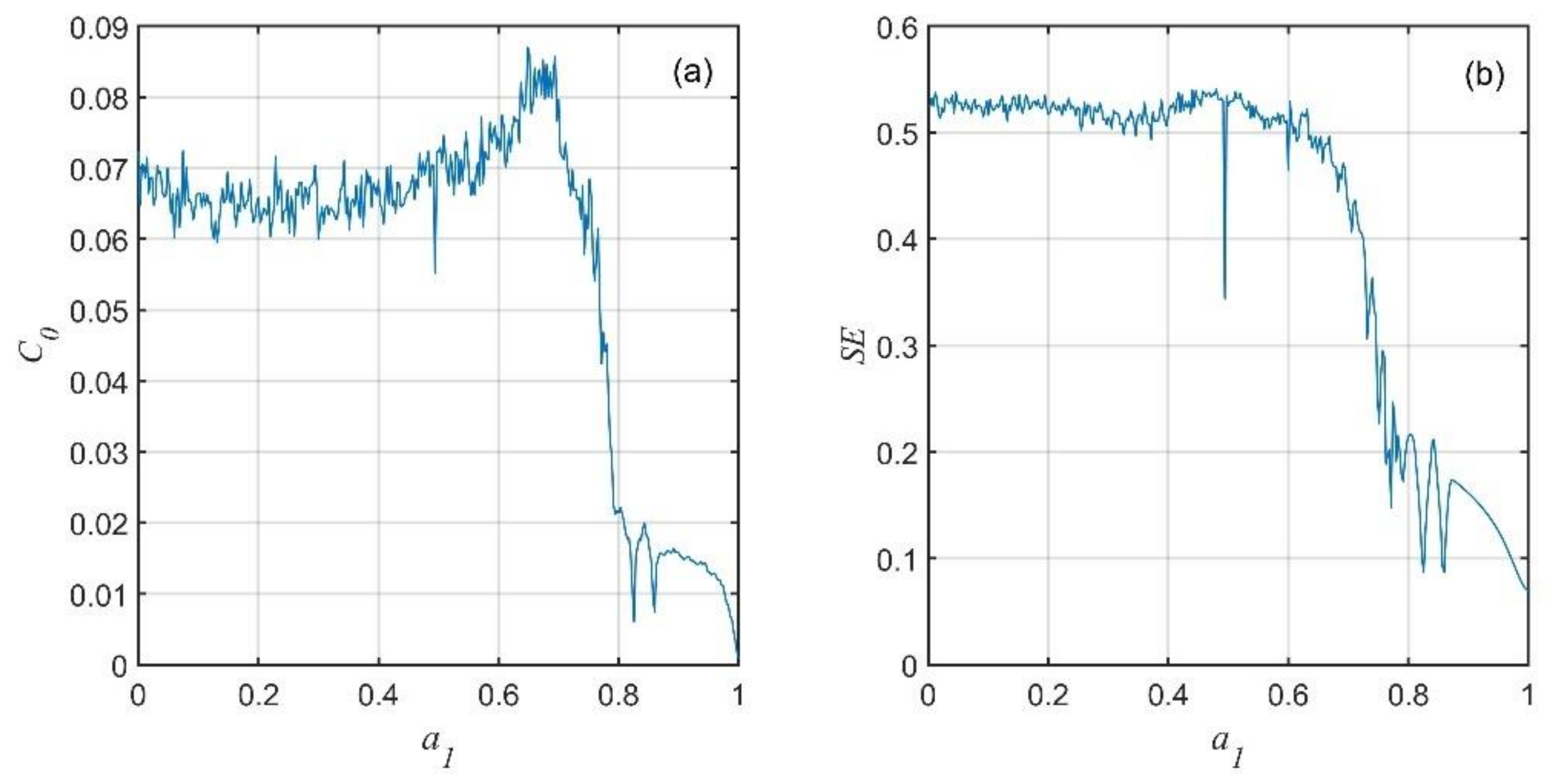
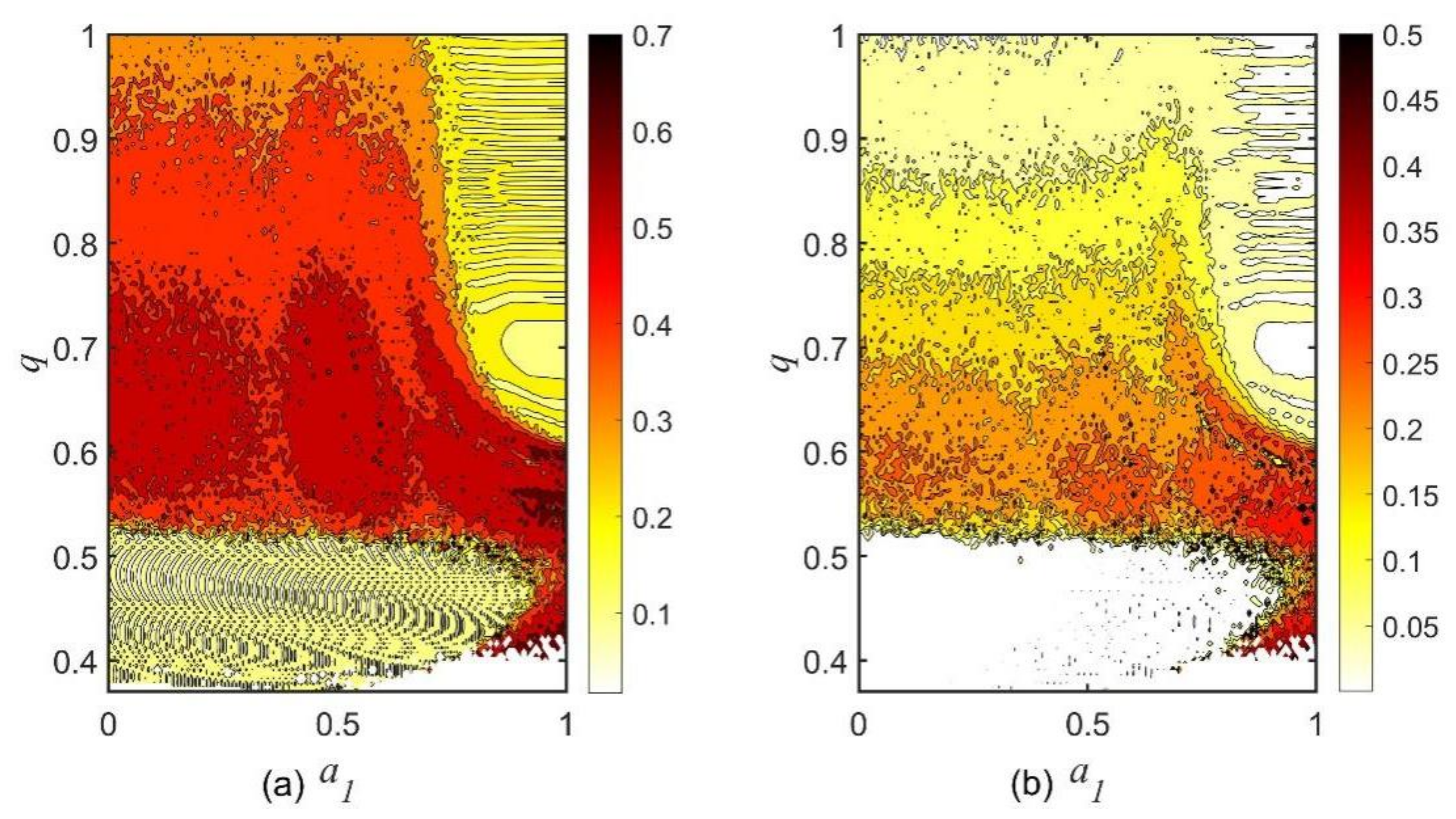
3.1. Dynamics of the Financial System with the Variation in the Parameter $a_1$

In order to study the influence of parameter $a_1$ on the dynamic behaviors of the financial system (14), we take the parameter values $a_2=a_3=0.1$, fractional-order $q=0.95$ and initial state $(x_0,y_0,z_0)$$=(1,3,2)$, and choose parameter $a_1$ as the critical variable. Figure 1 is the bifurcation diagram, which shows rich dynamic behaviors as $a_1$ changes within the interval $[0,1]$; the diagram implies that system (14) shows inverse period-doubling bifurcation, that is, the system goes from periodic states to chaotic states with the period-doubling bifurcation process, as the parameter $a_1$ decreases within the interval $[0,1]$. Specifically, the system is in period one when $a_1\in [0.9,1]$, and then period-doubling bifurcation occurs for $a_1=0.9$; period-two appears when $a_1\in [0.83,0.9)$, and period-doubling bifurcation occurs for $a_1=0.83$. As the parameter $a_1$ decreases from 0.7 to 0, the system is always in a state of chaos. Figure 2, showing the maximum Lyapunov exponent diagram, is an important component when exploring chaotic characteristics, where $a_1$ varies from 0 to 1. As presented in Figure 3, the $C_0$ and SE complexity values of system (14) are low for $a_1\in [0.7,1]$, while the complexity fluctuates around higher values for $a_1\in [0,0.7)$. The results in Figure 2 and Figure 3 are consistent with the bifurcation diagram.

Taking some values of $a_1$ to view the dynamic properties of system (14) more directly, Figure 4 presents the phase portraits and the $p-s$ plots of the $0-1$ testing of the system for some different values of parameter $a_1$. System (14) is in a chaotic state when $a_1=0.3$, and the chaotic attractor is shown in Figure 4a. In Figure 4b, system (14) appears in period two when $a_1$ rises to 0.85, which implies that the stability of the system is improved. From Figure 4c, we can see that the system is in period one when $a_1=1$. Correspondingly, the $0–1$ testing algorithm is applied and the $p-s$ plots are figured in Figure 4d–f, thus the existence of chaos is further verified and it can be seen that the chaos of the system rises as the value of $a_1$ decreases. These numerical images are consistent with the bifurcation diagram, the maximum Lyapunov exponent diagram and the complexity diagram, which actually reflect the complex connections between the interest rate, the investment demand and the price index of the financial system.

If the financial system (14) is in a periodic state, then the interest rate, investment demand and price index would show periodic oscillation in a certain range. As the amount of savings decreases, the financial system (14) enters into chaos, and this is often harmful for the actual financial system; it may be accompanied by financial crises and an uncontrolled financial system, and it will have damaging effects on the whole national economy. Therefore, it is necessary to keep the amount of savings at an appropriate level. Through the effective and appropriate control of such parameters by the government, the financial system will evolve into a more orderly state.

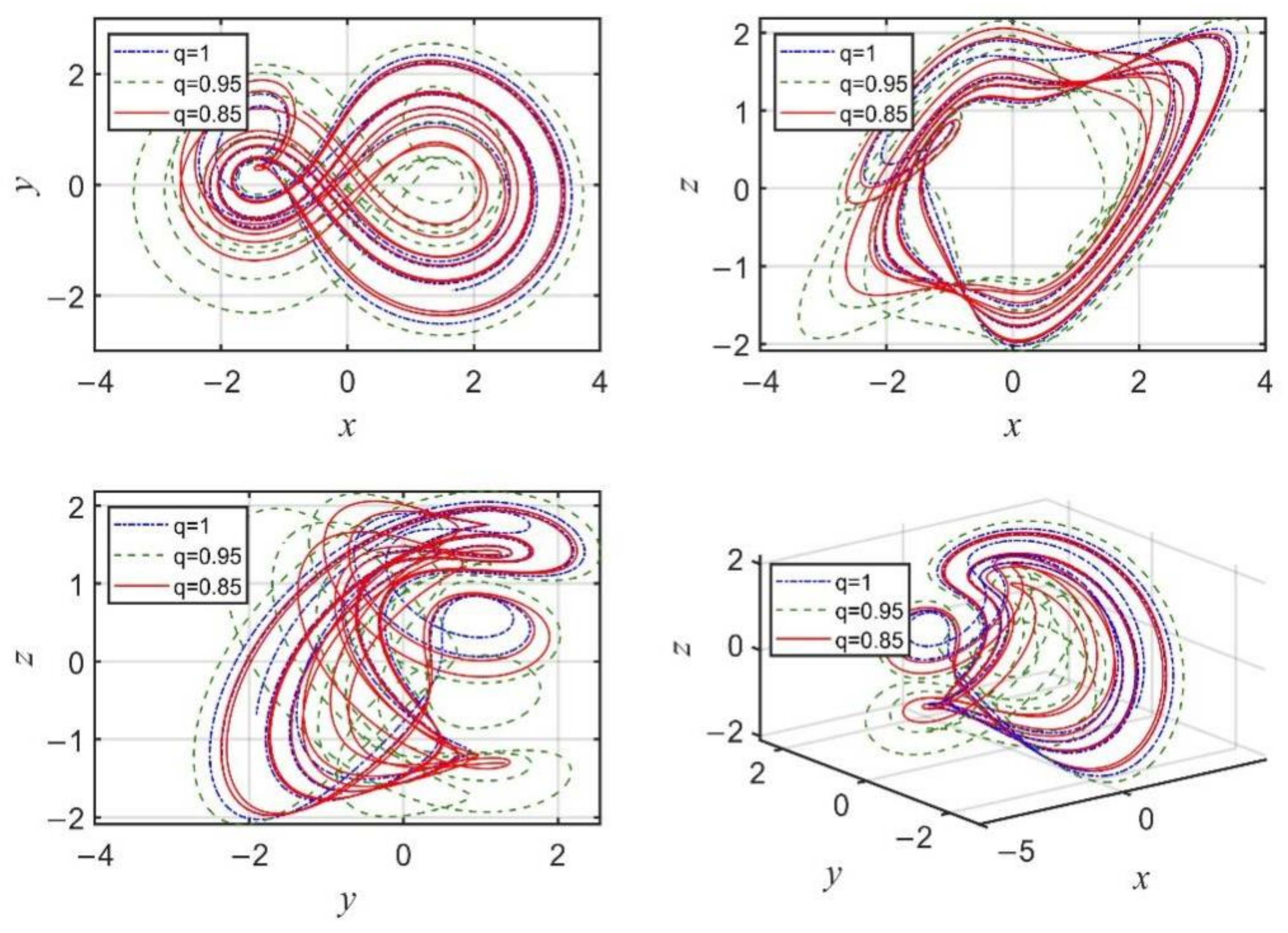
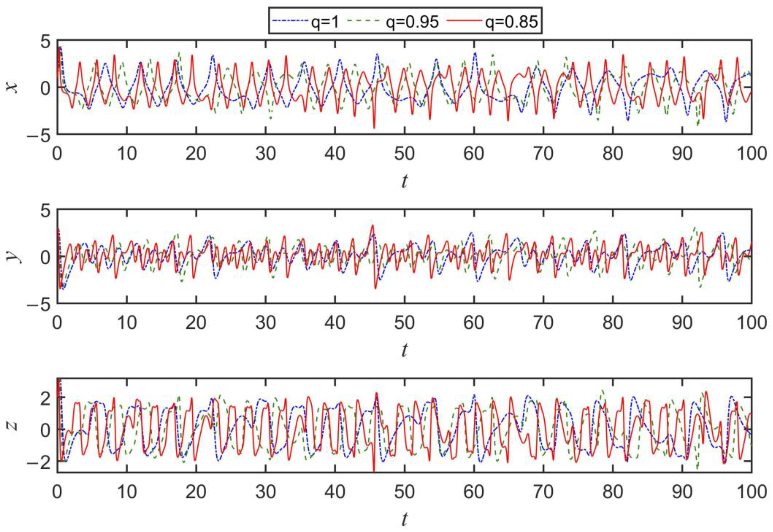
3.2. Dynamics of the Financial System with the Variation in the Fractional Order $q$

In order to analyze the effects of fractional order variation on system (14), let the parameters $a_1=0.3,a_2=a_3=0.1$ and the initial state $\left(x_0,y_0,z_0\right)=\left(1,3,2\right)$, and the fractional-order $q$ is chosen as the control variable. The bifurcation diagram with respect to $q$ within the interval $[0.37,1)$ is shown in Figure 5. The system is in periodic states for $q\in [0.37,0.51]$, and the system is sustainably in chaotic states while $q\in (0.51,1)$. Correspondingly, the maximum Lyapunov exponent diagram and the complexity diagram illustrate consistent results with the bifurcation diagram, which are shown in Figure 6 and Figure 7. In Figure 6, $q$ varies from 0.37 to 1. Figure 7 demonstrates that the $C_0$ and SE complexity values of system (14) are low for $q\in [0.37,0.51]$, and the complexity oscillates at higher values for $q\in (0.51,1)$. In Figure 8, the values of complexity change as $q$ and $a_1$ vary; darker colors represent larger values of complexity, and the chaos is mainly in the region with large values of $q$ and small values of $a_1$.

Figure 9 illustrates the $p–s$ plots of $0–1$ testing, which verify the chaos of the system (14) with some different values of $q$. More visually, Figure 10 shows the evolution of the interest rate, the investment demand and the price index of system (14), which display complex interactions with each other and vary with fractional orders. Figure 11 is a time series diagram of three state variables of different orders.

From the figures, it is easy to see that both the fractional-order and the saving amount affect the financial system. In fact, when the amount of savings in the financial system is determined, the system gradually moves from order to chaos as the fractional-order increases. When the fractional-order is determined, the financial system gradually moves from the chaos region to the order region as the amount of savings increases. Therefore, high order and low savings can complicate the financial system and make financial markets unstable and unpredictable. On the other hand, if the financial system is in a state of chaos, the financial markets would be out of control. For the government, instability and complexity make it difficult to give accurate economic forecasts, and impossible to predict the future state of the financial markets for a long time; therefore, it is important to achieve the goal of avoiding and removing chaos in fractional-order financial systems.

4. Fixed-Time Synchronization of Fractional-Order Chaotic Financial Systems

The analysis in Section 3 shows that the fractional-order financial system will be in a chaotic state when the value of the saving amount is low, and the trajectories of two financial systems with different initial conditions will exhibit different behaviors if an appropriate synchronization controller is not applied. To achieve the fixed-time synchronization between two chaotic financial systems, we design a synchronization controller and an adaptive parameter update law, which can be used to synchronize two chaotic financial systems and identify the unknown parameters respectively in the setting time, which does not depend on the initial conditions.

Consider the following nonlinear fractional-order system:

$${}_{t_0}{}^{C}D{}_t^q\mathbf{x}(t)=F(t,\mathbf{x}(t),\Theta )=f(t,\mathbf{x}(t))+g(t,\mathbf{x}(t))\Theta ,$$

(15)

where $f(t,\mathbf{x}(t))$ and $g(t,\mathbf{x}(t))$ are the sum of the two parts of $F(t,\mathbf{x}(t),\Theta )$, $\mathbf{x}(t)={\left(x_1(t),x_2(t),\dots ,x_n(t)\right)}^{{\rm T}}\in {ℝ}^n$ is the state vector, $\Theta ={\left({\Theta }_1,{\Theta }_2,\cdots ,{\Theta }_m\right)}^T\in {ℝ}^m$ is the unknown parameter vector, $f(t,\mathbf{x}(t)):{ℝ}^{+}\times {ℝ}^n\to {ℝ}^n$ is the continuous function vector, and $g(t,\mathbf{x}(t)):{ℝ}^{+}\times {ℝ}^n\to {ℝ}^{n\times m}$ is the continuous function matrix, $0<q<1$, $t_0\ge 0$.

The following fractional-order chaotic system as the driving system is presented as

$${}_{t_0}{}^{C}D{}_t^q\mathbf{x}(t)=F(t,\mathbf{x}(t),\Theta ),$$

(16)

where $0<q<1$; $\mathbf{x}(t)={\left(x_1(t),x_2(t),\cdots ,x_n(t)\right)}^{{\rm T}}\in {ℝ}^n$ denotes the drive state vector, and the controlled response system is given by

$${}_{t_0}{}^{C}D{}_t^q\mathbf{y}(t)=F(t,\mathbf{y}(t),\widehat{\Theta }(t))+\mathbf{u}(t),$$

(17)

where $0<q<1$; $\mathbf{y}(t)={\left(y_1(t),y_2(t),\cdots ,y_n(t)\right)}^{{\rm T}}\in {ℝ}^n$ denotes the response state vector, and $\widehat{\Theta }(t)$ is the estimation of the unknown parameter $\Theta$. Then, the estimation error of unknown parameter $\tilde{\Theta }(t)=\widehat{\Theta }(t)-\Theta$. $\mathbf{u}(t)={\left(u_1(t),u_2(t),\cdots ,u_n(t)\right)}^{{\rm T}}\in {ℝ}^n$ is the synchronization controller, to be designed later.

We denote the error variables as $\mathbf{e}(t)=\mathbf{y}(t)-\mathbf{x}(t)$, where $\mathbf{e}(t)=\left(e_1(t),e_2(t),\dots ,\right.$${\left.e_n(t)\right)}^{{\rm T}}\in {ℝ}^n$, and then the fractional-order error system is obtained as

$$\begin{gathered} {}_{t_0}{}^{C}D{}_t^q\mathbf{e}(t)=F(t,\mathbf{y}(t),\widehat{\Theta }(t))-F(t,\mathbf{x}(t),\Theta )+\mathbf{u}(t) \\ =F(t,\mathbf{y}(t),\Theta (t))-F(t,\mathbf{x}(t),\Theta )+g(t,\mathbf{y}(t))(\widehat{\Theta }(t)-\Theta )+\mathbf{u}(t). \end{gathered}$$

(18)

The next assumption and lemma are helpful for the analysis in the following Section 4.1.

Assumption 1

. For any$\mathbf{x}(t)$,$\mathbf{y}(t)$$\in {ℝ}^n$,$F(t,\mathbf{x}(t))$and$F(t,y(t))$are Lipschitz continuous, and there exists a matrix$L={(l_{ij})}_{n\times n}$in which$l_{ij}\ge 0$, such that

$$\left|F_i(t,\mathbf{y}(t))-F_i(t,\mathbf{x}(t))\right|\le {\displaystyle \sum _{j=1}^n{l}_{ij}\left|{\mathbf{y}}_j(t)-{\mathbf{x}}_j(t)\right|}, i=1,2,\cdots ,n.$$

Lemma 3

[57]. If $f(t)\in C^1([t_0,+\infty ),ℝ)$ is a continuously differentiable function, then

$${}_{t_0}{}^{C}D{}_t^q\left|f(t)\right|\le sign(f(t)){}_{t_0}{}^{C}D{}_t^{q}f(t),0<q<1.$$

Lemma 4

[58]. If $z_1,z_2,\cdots ,z_n>0$,$r>1$ and$0<l\le 1$, then the following inequalities hold,

$${\displaystyle \sum _{i=1}^n{z}_i^r}\ge n^{1-r}{\left({\displaystyle \sum _{i=1}^n{z}_i}\right)}^r, {\displaystyle \sum _{i=1}^n{z}_i^l}\ge {\left({\displaystyle \sum _{i=1}^n{z}_i}\right)}^l.$$

Lemma 5

[47]. For a fractional-order system ${}_{t0}{D}_t^q=f(t,x(t))$, the origin is fixed-time stable if there exists a positive definite function$V(t,x(t))\triangleq V(t)$, such that

$${}_0{D}_t^{q}V(t)\le \frac{{\lambda }_1\Gamma (1-\gamma )}{\Gamma (2-q)\Gamma (q-\gamma +1)}{V}^{1-q+\gamma }(t)-\frac{{\lambda }_2\Gamma (1-\varpi )}{\Gamma (2-q)\Gamma (q-\varpi +1)}{V}^{1-q+\varpi }(t)$$

(19)

with ${\lambda }_1>0$, ${\lambda }_2>0$, $1<\gamma <q+1$ and $q-1<\varpi <q$. The setting time is estimated by

$$T={\left(\frac{\Gamma (1+q)}{{\lambda }_1}\right)}^{\frac{1}{q}}+{\left(\frac{\Gamma (1+q)}{{\lambda }_2}\right)}^{\frac{1}{q}},$$

(20)

which is independent of the initial conditions.

4.1. Fixed-Time Synchronization Implementation

Let system (14) be the drive financial system, and the response financial system is correspondingly given as follows:

$$\left\{\begin{array}{c}{}_0{}^{C}D{}_t^q{x}_1=-{\widehat{a}}_1{x}_1+z_1+x_1{y}_1+u_1(t)\\ {}_0{}^{C}D{}_t^q{y}_1=2-{\widehat{a}}_2{y}_1-x_1{}^2+u_2(t)\\ {}_0{}^{C}D{}_t^q{z}_1=-x_1-{\widehat{a}}_3{z}_1+x_1{y}_1+u_3(t)\end{array}\right.,$$

(21)

where ${\widehat{a}}_1$,${\widehat{a}}_2$ and ${\widehat{a}}_3$ are the estimations of the unknown parameters $a_1$,$a_2$ and $a_3$.

The estimation errors of unknown parameters are as follows: ${\tilde{a}}_1={\widehat{a}}_1-a_1$,${\tilde{a}}_2={\widehat{a}}_2-a_2$ and ${\tilde{a}}_3={\widehat{a}}_3$$-a_3$, and the synchronization error is defined as $e_1=x_1-x$,$e_2=y_1-y$ and $e_3=z_1-z$.

The controller is designed as follows:

$$\left\{\begin{array}{c}{u}_1(t)=-l{e}_1(t)-m_{11}{e}_1(t){\left|e_1(t)\right|}^{\alpha }-m_{21}{e}_1(t){\left|e_1(t)\right|}^{\beta }\\ u_2(t)=-l{e}_2(t)-m_{12}{e}_2(t){\left|e_2(t)\right|}^{\alpha }-m_{22}{e}_2(t){\left|e_2(t)\right|}^{\beta }\\ u_3(t)=-l{e}_3(t)-m_{13}{e}_3(t){\left|e_3(t)\right|}^{\alpha }-m_{23}{e}_3(t){\left|e_3(t)\right|}^{\beta }\end{array}\right.,$$

(22)

and the adaptive update law of estimated parameters is designed as

$$\left\{\begin{array}{cc}{}_{t_0}^C{D}_t^q{\widehat{a}}_1=& -max\left\{\left|x_1\right|,\left|y_1\right|,\left|z_1\right|\right\}\left({\tilde{a}}_1\right)-m_{11}{\tilde{a}}_1{\left|{\tilde{a}}_1\right|}^{\alpha }-m_{21}{\tilde{a}}_1{\left|{\tilde{a}}_1\right|}^{\beta }\\ {}_{t_0}^C{D}_t^q{\widehat{a}}_2=& -max\left\{\left|x_1\right|,\left|y_1\right|,\left|z_1\right|\right\}\left({\tilde{a}}_2\right)-m_{12}{\tilde{a}}_2{\left|{\tilde{a}}_2\right|}^{\alpha }-m_{22}{\tilde{a}}_2{\left|{\tilde{a}}_2\right|}^{\beta }\\ {}_{t_0}^C{D}_t^q{\widehat{a}}_3=& -max\left\{\left|x_1\right|,\left|y_1\right|,\left|z_1\right|\right\}\left({\tilde{a}}_3\right)-m_{13}{\tilde{a}}_3{\left|{\tilde{a}}_3\right|}^{\alpha }-m_{23}{\tilde{a}}_3{\left|{\tilde{a}}_3\right|}^{\beta }\end{array}\right.,$$

(23)

where $l>0$ is the control gain, and $m_{1i}$ and $m_{2i}$ $(i=1,2,3)$ are adjustable positive constants.

Then, the fractional-order error system can be obtained by subtracting the drive financial system (14) from the response financial system (21), which is given by

$$\left\{\begin{array}{c}{}_0^C{D}_t^q{e}_1=-0.3e_1+e_3+x_1{e}_2+y{e}_1-x_1\left({\tilde{a}}_1\right)-l{e}_1-m_{11}{e}_1\left(t\right){\left|e_1\left(t\right)\right|}^{\alpha }-m_{21}{e}_1\left(t\right){\left|e_1\left(t\right)\right|}^{\beta }\\ {}_0^C{D}_t^q{e}_2=-0.1e_2-(x+x_1)e_1-y_1\left({\tilde{a}}_2\right)-l{e}_2-m_{12}{e}_2\left(t\right){\left|e_2\left(t\right)\right|}^{\alpha }-m_{22}{e}_2\left(t\right){\left|e_2\left(t\right)\right|}^{\beta }\\ {}_0^C{D}_t^q{e}_3=-e_1-0.1e_3+x_1{e}_2+y{e}_1-z_1\left({\tilde{a}}_3\right)-l{e}_3-m_{13}{e}_3\left(t\right){\left|e_3\left(t\right)\right|}^{\alpha }-m_{23}{e}_3\left(t\right){\left|e_3\left(t\right)\right|}^{\beta }\end{array}\right.$$

(24)

The main result is stated as follows.

Theorem 

1. Under Assumption 1, the controller (22) and the adaptive law (23), if there exists a constant$l$that satisfies

$$l\ge \max \left\{{\displaystyle \sum _{i=1}^3{l}_{ij},j=1,2,3}\right\},$$

(25)

and$1-q<\alpha <1$,$-1<\beta <0$,$m_{1i}>0$, and$m_{2i}>0$$(i=1,2,3)$, then the drive system (14) and the response system (21) can be synchronized, and the unknown parameters$a_1$,$a_2$and$a_3$can also be successfully identified as${\widehat{a}}_1$,${\widehat{a}}_2$and${\widehat{a}}_3$in fixed-time$T=$${\left(-\frac{\Gamma (1+q)\Gamma (1-q-\alpha )}{m_1\cdot 6^{-\alpha }\Gamma (2-q)\Gamma (1-\alpha )}\right)}^{\frac{1}{q}}+{\left(\frac{\Gamma (1+q)\Gamma (1-q-\beta )}{m_2\Gamma (2-q)\Gamma (1-\beta )}\right)}^{\frac{1}{q}}$, where$m_1={\min }_i\left\{m_{1i}\right\}$, and$m_2={\min }_i\left\{m_{2i}\right\}$.

Proof. 

We construct the Lyapunov function as

$$V(t)={\displaystyle \sum _{i=1}^3\left|e_i(t)\right|}+{\displaystyle \sum _{j=1}^3\left|{\tilde{a}}_j\right|}.$$

□

Calculating the Caputo fractional-order derivative of $V(t)$ and using Lemma 3, Assumption 1, the fractional-order error system (24) and the adaptive law (23), we obtain

$$\begin{gathered} {}_{t_0}{}^{C}D{}_t^{q}V(t)={}_{t_0}{}^{C}D{}_t^q\left({\displaystyle \sum _{i=1}^3\left|e_i(t)\right|}+{\displaystyle \sum _{j=1}^3\left|{\tilde{a}}_j\right|}\right) \\ \le {\displaystyle \sum _{i=1}^{3}sign(e_i(t)){}_{t_0}{}^{C}D{}_t^q{e}_i(t)}+{\displaystyle \sum _{j=1}^{3}sign({\tilde{a}}_j){}_{t_0}{}^{C}D{}_t^q({\tilde{a}}_j)} \\ ={\left(sign(\mathbf{e}(t))\right)}^T\left[\left(\begin{array}{c}-0.3e_1+e_3+x_1{e}_2+y{e}_1\\ -0.1e_2-(x_1+x)e_1\\ -e_1-0.1e_3+x_1{e}_2+y{e}_1\end{array}\right)\right. \\ +\left(\begin{array}{ccc}-x_1& 0& 0\\ 0& -y_1& 0\\ 0& 0& -z_1\end{array}\right)\left(\begin{array}{c}{\tilde{a}}_1\\ {\tilde{a}}_2\\ {\tilde{a}}_3\end{array}\right)-le(t) \\ -\left.\left(\begin{array}{c}{m}_{11}{e}_1(t){\left|e_1(t)\right|}^{\alpha }+m_{21}{e}_1(t){\left|e_1(t)\right|}^{\beta }\\ m_{12}{e}_2(t){\left|e_2(t)\right|}^{\alpha }+m_{22}{e}_2(t){\left|e_2(t)\right|}^{\beta }\\ m_{13}{e}_3(t){\left|e_3(t)\right|}^{\alpha }+m_{23}{e}_3(t){\left|e_3(t)\right|}^{\beta }\end{array}\right)\right] \\ +{\left(sign(\tilde{\Theta })\right)}^T\left[-\max \left\{\left|x_1\right|,\left|y_1\right|,\left|z_1\right|\right\}(\tilde{\Theta })-\left(\begin{array}{c}{m}_{11}{\tilde{a}}_1{\left|{\tilde{a}}_1\right|}^{\alpha }+m_{21}{\tilde{a}}_1{\left|{\tilde{a}}_1\right|}^{\beta }\\ m_{12}{\tilde{a}}_2{\left|{\tilde{a}}_2\right|}^{\alpha }+m_{22}{\tilde{a}}_2{\left|{\tilde{a}}_2\right|}^{\beta }\\ m_{13}{\tilde{a}}_3{\left|{\tilde{a}}_3\right|}^{\alpha }+m_{23}{\tilde{a}}_3{\left|{\tilde{a}}_3\right|}^{\beta }\end{array}\right)\right] \\ \begin{array}{c}\le \left|sign(e_1)\right|\left|-0.3e_1+e_3+x_1{e}_2+y{e}_1\right|\\ +\left|sign(e_2)\right|\left|-0.1e_2-(x_1+x)e_1\right|\\ +\left|sign(e_3)\right|\left|-e_1-0.1e_3+x_1{e}_2+y{e}_1\right|\\ +\max \left\{\left|x_1\right|,\left|y_1\right|,\left|z_1\right|\right\}{‖\tilde{\Theta }‖}_1\\ -l{\left(sign(e(t))\right)}^{T}e(t)-m_1\left({\displaystyle \sum _{i=1}^3{\left|e_i(t)\right|}^{\alpha +1}}+{\displaystyle \sum _{j=1}^3{\left|{\tilde{a}}_j\right|}^{\alpha +1}}\right)\\ -m_2\left({\displaystyle \sum _{i=1}^3{\left|e_i(t)\right|}^{\beta +1}}+{\displaystyle \sum _{j=1}^3{\left|{\tilde{a}}_j\right|}^{\beta +1}}\right)\\ -{\left(sign(\tilde{\Theta })\right)}^T\max \left\{\left|x_1\right|,\left|y_1\right|,\left|z_1\right|\right\}\left(\tilde{\Theta }\right)\end{array} \\ =\left|sign(e_1)\right|\left|-0.3e_1+e_3+x_2{e}_2+y_1{e}_1\right| \\ +\left|sign(e_2)\right|\left|-0.1e_2-(x+x_1)e_1\right| \\ +\left|sign(e_3)\right|\left|-e_1-0.1e_3+x_1{e}_2+y{e}_1\right| \\ \begin{array}{l}-l{\left(sign(e(t))\right)}^{T}e(t)-m_1\left({\displaystyle \sum _{i=1}^3{\left|e_i(t)\right|}^{\alpha +1}}+{\displaystyle \sum _{j=1}^3{\left|{\tilde{a}}_j\right|}^{\alpha +1}}\right)\\ -m_2\left({\displaystyle \sum _{i=1}^3{\left|e_i(t)\right|}^{\beta +1}}+{\displaystyle \sum _{j=1}^3{\left|{\tilde{a}}_j\right|}^{\beta +1}}\right)\end{array} \\ \le {\displaystyle \sum _{i=1}^3{\displaystyle \sum _{k=1}^3{l}_{ik}\left|e_k(t)\right|}}-{\displaystyle \sum _{k=1}^{3}l\left|e_k(t)\right|}-m_1\left({\displaystyle \sum _{i=1}^3{\left|e_i(t)\right|}^{\alpha +1}}+{\displaystyle \sum _{j=1}^3{\left|{\tilde{a}}_j\right|}^{\alpha +1}}\right) \\ -m_2\left({\displaystyle \sum _{i=1}^3{\left|e_i(t)\right|}^{\beta +1}}+{\displaystyle \sum _{j=1}^3{\left|{\tilde{a}}_j\right|}^{\beta +1}}\right). \end{gathered}$$

From the condition (25) and Lemma 4, we get

$$\begin{gathered} {}_{t_0}{}^{C}D{}_t^{q}V(t)\le -m_1\left({\displaystyle \sum _{i=1}^3{\left|e_i(t)\right|}^{\alpha +1}}+{\displaystyle \sum _{j=1}^3{\left|{\tilde{a}}_j\right|}^{\alpha +1}}\right)-m_2\left({\displaystyle \sum _{i=1}^3{\left|e_i(t)\right|}^{\beta +1}}+{\displaystyle \sum _{j=1}^3{\left|{\tilde{a}}_j\right|}^{\beta +1}}\right) \\ \le -m_1\cdot 6^{-\alpha }{\left({\displaystyle \sum _{i=1}^3\left|e_i(t)\right|}+{\displaystyle \sum _{j=1}^3\left|{\tilde{a}}_j\right|}\right)}^{\alpha +1}-m_2{\left({\displaystyle \sum _{i=1}^3\left|e_i(t)\right|}+{\displaystyle \sum _{j=1}^3\left|{\tilde{a}}_j\right|}\right)}^{\beta +1} \\ =-m_1\cdot 6^{-\alpha }{V}^{\alpha +1}(t)-m_2{V}^{\beta +1}(t). \end{gathered}$$

According to Lemma 5, we choose ${\lambda }_1=\frac{-m_1\cdot 6^{-\alpha }\Gamma (2-q)\Gamma (q-\gamma +1)}{\Gamma (1-\gamma )}$, ${\lambda }_2=$ $\frac{m_2\Gamma (2-q)\Gamma (q-\varpi +1)}{\Gamma (1-\varpi )}$, $\alpha +1=1-q+\gamma$ and $\beta +1=1-q+\varpi$, and then we have $V(t)=0$, i.e., $e_1=e_2=e_3=0$ and ${\tilde{a}}_1=0$, ${\tilde{a}}_2=0$, ${\tilde{a}}_3=0$, $\forall t\ge T$. That means the synchronization between the drive system (14) and the response system (21) can be realized within the fixed time $T={\left(\frac{-\Gamma (1+q)\Gamma (1-q-\alpha )}{m_1\cdot 6^{-\alpha }\Gamma (2-q)\Gamma (1-\alpha )}\right)}^{\frac{1}{q}}+{\left(\frac{\Gamma (1+q)\Gamma (1-q-\beta )}{m_2\Gamma (2-q)\Gamma (1-\beta )}\right)}^{\frac{1}{q}}$, and the unknown parameters can also be identified in fixed time $T$. The proof is completed.

4.2. Numerical Simulation

The illustrative examples are provided to show the effectiveness of the results obtained. The fixed-time synchronization of the drive system (14) and the response system (21) with different initial states for some different fractional orders are studied. In order to ensure that (14) and (21) are in a chaotic state, we take the fractional orders $q=0.95$, $q=0.9$, and $q=0.85$, respectively, and choose the system parameters $a_1=0.3$, $a_2=$ $a_3=0.1$ according to the dynamic analysis in Section 3. The initial state values of the drive system $\left(x_1(0),y_1(0),z_1(0)\right)$$=(1,3,2)$, the response system $\left(x_2(0),y_2(0),z_2(0)\right)$$=(2,1,3)$, and $\widehat{\Theta }(0)={(1,2,3)}^T$. From the phase portrait, we can determine that $\left|x\right|<4.5$, $\left|y\right|<3.5$, $\left|z\right|<2.8$; then, according to Assumption 1, we can easily get the matrix $L=\left(\begin{array}{ccc}3.2& 4.5& 1\\ 9& 0.1& 0\\ 2.5& 4.5& 0.1\end{array}\right)$.

Based on Theorem 1, let $l=14.8>\max \left\{{\displaystyle \sum _{i=1}^3{l}_{ij},j=1,2,3}\right\}$ $=14.7$, and the other parameters in (22) and (23) are chosen as $m_{11}=m_{21}=5$, $m_{12}=m_{22}=8$, $m_{13}=$ $m_{23}=8$, $\alpha =0.35$ and $\beta =-0.05$; then we have $m_1=m_2=5$. We obtain the setting times ${\left.T\right|}_{q=0.95}=3.2264$, ${\left.T\right|}_{q=0.9}=2.7134$, and ${\left.T\right|}_{q=0.85}=2.6805$.

As shown in Figure 12 and Figure 13, the synchronization errors obviously eventually converge to zero, and the unknown parameters are successfully identified within the fixed times ${\left.T\right|}_{q=0.95}$, ${\left.T\right|}_{q=0.9}$ and ${\left.T\right|}_{q=0.85}$ for these different fractional orders, respectively. This demonstrates that the two chaotic financial systems realize fixed-time synchronization under the designed controller. Meanwhile, for the fractional-order control systems, the setting time of fixed-time stability depends not only on the parameters of the controller, but also on the order of the fractional-order derivative. Moreover, the fixed-time synchronization between (14) and (21) is achieved faster as the fractional derivative order decreases. The numerical simulation illustrates the effectiveness of fixed-time synchronization controller designed, and it implies that the interest rate, the investment demand and the price index in chaotic financial systems can be synchronized within a fixed time with an appropriate synchronization controller.

Synchronization between two financial systems helps maintain the consistency between these two financial systems. That is to say, achieving synchronization implies that two financial systems in different regions and countries still maintain similar dynamic behaviors. From the economic point of view, the drive economic system can be regarded as the intended economic objective, while the response system is forced to achieve this goal. The fractional order has an important impact on the time required to achieve the synchronization of the financial systems, and we all want the financial system to reach the desired goal as soon as possible, independent of the differences in initial economic conditions. Therefore, achieving chaos synchronization under a realistic assumption of the drive economic system with an appropriate fractional order is of great significance.

Based on the above analysis, analyzing the fixed-time synchronization of the proposed fractional-order financial models without considering the initial economic gap between the two economies is useful for control, regulation, and maintaining consistency between two asynchronous financial systems.

5. Conclusions

In this paper, we establish a fractional-order financial system with the Caputo derivative, and the numerical solutions are obtained by ADM. The complex interactions and dynamic behaviors are analyzed by numerical tools and methods. Both the system parameter and the fractional order can be taken as bifurcation parameters, which show that the fractional-order financial model has complex and abundant dynamics. In particular, chaotic behavior in the financial system is unfavorable to the market, and must be controlled. Thus, based on the properties of fractional calculus and some analysis techniques, the control scheme is designed to achieve fixed-time synchronization and parameter identification in fractional-order financial systems, where the setting time of synchronization is independent of the initial conditions. Finally, numerical simulations indicate that the proposed controlling scheme is effective and feasible. The results can help to improve the understanding of the dynamic behaviors of financial system, and provide theoretical support for the formulation of financial intervention strategies.

Since time lag [22,25] is an important factor leading to instability in the financial system, studying a financial system with time lags plays an important role in understanding and managing financial markets. As such, our future works will focus on this issue.

References

1. Yuan, L.; Yang, Q. Parameter identification and synchronization of fractional-order chaotic systems. Commun. Nonlinear Sci. Numer. Simul. 2012, 17, 305–316. [Google Scholar] [CrossRef]
2. Yuan, L.; Zheng, S.; Alam, Z. Dynamics analysis and cryptographic application of fractional logistic map. Nonlinear Dyn. 2019, 96, 615–636. [Google Scholar] [CrossRef]
3. Chen, L.; Yin, H.; Huang, T.; Yuan, L.; Zheng, S.; Yin, L. Chaos in fractional-order discrete neural networks with application to image encryption. Neural Netw. 2020, 125, 174–184. [Google Scholar] [CrossRef] [PubMed]
4. He, Y.; Zheng, S.; Yuan, L. Dynamics of fractional-order digital manufacturing supply chain system and its control and synchronization. Fractal Fract. 2021, 5, 128. [Google Scholar] [CrossRef]
5. Cafagna, D.; Grassi, G. Bifurcation and chaos in the fraction-order Chen system via time-domain approach. Int. J. Bifurc. Chaos 2008, 18, 1845–1863. [Google Scholar] [CrossRef]
6. Tavazoei, M.; Asemani, M. On Robust stability of incommensurate fractional-order systems. Commun. Nonlinear Sci. Numer. Simul. 2020, 90, 105344. [Google Scholar] [CrossRef]
7. Wang, J.; Mou, J.; Xiong, L.; Zhang, Y.; Cao, Y. Fractional-order design of a novel non-autonomous laser chaotic system with compound nonlinearity and its circuit realization. Chaos Solitons Fractals 2021, 152, 111324. [Google Scholar] [CrossRef]
8. Mahmoud, E.E.; Trikha, P.; Jahanzaib, L.S.; Almaghrabi, O.A. Dynamic analysis and chaos control of the fractional chaotic ecological model. Chaos Solitons Fractals 2020, 141, 110348. [Google Scholar] [CrossRef]
9. Debbouche, N.; Almatroud, A.O.; Ouannas, A.; Batiha, I.M. Chaos and coexisting attractors in glucose-insulin regulatory system with incommensurate fractional-order derivatives. Chaos Solitons Fractals 2021, 143, 110575. [Google Scholar] [CrossRef]
10. Ma, J.; Chen, Y. Study for the bifurcation topological structure and the global complicated character of a kind of nonlinear finance system (I). Appl. Math. Mech. 2001, 22, 1240–1251. [Google Scholar] [CrossRef]
11. Ma, J.; Chen, Y. Study for the bifurcation topological structure and the global complicated character of a kind of nonlinear finance system (II). Appl. Math. Mech. 2001, 22, 1375–1382. [Google Scholar] [CrossRef]
12. Yu, H.; Cai, G.; Li, Y. Dynamic analysis and control of a new hyperchaotic finance system. Nonlinear Dyn. 2012, 67, 2171–2182. [Google Scholar] [CrossRef]
13. Cai, G.; Yao, L.; Hu, P.; Fang, X. Adaptive full state hybrid function projective synchronization of financial hyperchaotic systems with uncertain parameters. Discret. Contin. Dyn. Syst.-Ser. B 2017, 18, 2019–2028. [Google Scholar] [CrossRef]
14. Jin, S.; Zhao, L. Complexity analysis of a four-dimensional energy-Economy-environment dynamic system. Complexity 2020, 2020, 7626792. [Google Scholar] [CrossRef]
15. Gholamin, P.; Sheikhani, A. Dynamic analysis of a new three-dimensional fractional chaotic system. Pramana 2019, 92, 91. [Google Scholar] [CrossRef]
16. Zhang, X.; Zhu, H.; Sahoo, A. Hopf bifurcation and chaos of a delayed finance System. Complexity 2019, 2019, 6715036. [Google Scholar] [CrossRef]
17. Peters, E.E. Fractal Market Analysis: Applying Chaos Theory to Investment and Economics; Wiley: New York, NY, USA, 1994; pp. 39–64. [Google Scholar]
18. Granger, C.W.J.; Joyeux, R. An introduction to long memory time series models and fractional differencing. Time Ser. 1980, 1, 15–39. [Google Scholar] [CrossRef]
19. Baillie, R.N. Long memory processes and fractional integration in econometrics. J. Econom. 1996, 73, 5–59. [Google Scholar] [CrossRef]
20. Xin, B.; Li, Y. 0-1 test for chaos in a fractional order financial system with investment incentive. Abstr. Appl. Anal. 2013, 2013, 876298. [Google Scholar] [CrossRef]
21. Xu, S.; Lv, H.; Liu, H.; Liu, A. Robust control of disturbed fractional-order economical chaotic systems with uncertain parameters. Complexity 2019, 2019, 7567695. [Google Scholar] [CrossRef] [Green Version]
22. Zhang, Z.; Zhang, J.; Cheng, F.; Xu, Y. Bifurcation analysis and stability criterion for the nonlinear fractional-order three-dimensional financial system with delay. Asian J. Control 2019, 21, 1–11. [Google Scholar] [CrossRef]
23. Wang, S.; He, S.; Yousefpour, A.; Jahanshahi, H.; Repnik, R.; Perc, M. Chaos and complexity in a fractional-order financial system with time delays. Chaos Solitons Fractals 2020, 131, 109521. [Google Scholar] [CrossRef]
24. Chu, Y.M.; Bekiros, S.; Zambrano-Serrano, E.; Orozco-López, O.; Lahmiri, S.; Jahanshahi, H.; Aly, A.A. Artificial macro-economics: A chaotic discrete-time fractional-order laboratory model. Chaos Solitons Fractals 2021, 145, 110776. [Google Scholar] [CrossRef]
25. Lin, Z.; Wang, H. Modeling and application of fractional-order economic growth model with time delay. Fractal Fract. 2021, 5, 74. [Google Scholar] [CrossRef]
26. Jahanshahi, H.; Sajjadi, S.S.; Bekiros, S.; Aly, A.A. On the development of variable-order fractional hyperchaotic economic system with a nonlinear model predictive controller. Chaos Solitons Fractals 2021, 144, 110698. [Google Scholar] [CrossRef]
27. Zhang, Y.; Du, Y. Synchronization Problem of a novel fractal-fractional orders’ hyperchaotic finance system. Math. Probl. Eng. 2021, 2021, 4152160. [Google Scholar] [CrossRef]
28. Hajipour, A.; Hajipour, M.; Baleanu, D. On the adaptive sliding mode controller for a hyperchaotic fractional-order financial system. Phys. A Stat. Mech. Its Appl. 2018, 497, 139–153. [Google Scholar] [CrossRef]
29. Liping, C.; Khan, M.A.; Atangana, A.; Kumar, S. A new financial chaotic model in Atangana-Baleanu stochastic fractional differential equations. AEJ-Alex. Eng. J. 2021, 60, 5193–5204. [Google Scholar] [CrossRef]
30. Shi, J.; He, K.; Fang, H. Chaos, Hopf bifurcation and control of a fractional-order delay financial system. Math. Comput. Simul. 2022, 194, 348–364. [Google Scholar] [CrossRef]
31. Jahanshahi, H.; Shahriari-Kahkeshi, M.; Alcaraz, R.; Wang, X.; Singh, V.P.; Pham, V.T. Entropy analysis and neural network-based adaptive control of a non-equilibrium four-dimensional chaotic system with hidden attractors. Entropy 2019, 21, 156. [Google Scholar] [CrossRef] [Green Version]
32. Zheng, S. Parameter identification and adaptive impulsive synchronization of uncertain complex-variable chaotic systems. Nonlinear Dyn. 2013, 74, 957–967. [Google Scholar] [CrossRef]
33. Zheng, S. Stability of uncertain impulsive complex-variable chaotic systems with time varying delays. ISA Trans. 2015, 58, 20–26. [Google Scholar] [CrossRef] [PubMed]
34. Zheng, S. Synchronization analysis of time delay complex-variable chaotic systems with discontinuous coupling. J. Frankl. Inst. 2016, 353, 1460–1477. [Google Scholar] [CrossRef]
35. Chen, H.; Yu, L.; Wang, Y.; Guo, M. Synchronization of a hyperchaotic finance System. Complexity 2021, 2021, 6618435. [Google Scholar] [CrossRef]
36. Tacha, O.I.; Volos, C.K.; Kyprianidis, I.M.; Stouboulos, I.N.; Vaidyanathan, S.; Pham, V.T. Analysis, adaptive control and circuit simulation of a novel nonlinear finance system. Appl. Math. Comput. 2016, 276, 200–217. [Google Scholar] [CrossRef]
37. Rao, R.; Zhu, Q. Exponential synchronization and stabilization of delayed feedback hyperchaotic financial system. Adv. Differ. Equ. 2021, 2021, 216. [Google Scholar] [CrossRef]
38. Zheng, S. Further Results on the impulsive synchronization of uncertain complex-variable chaotic delayed systems. Complexity 2016, 21, 131–142. [Google Scholar] [CrossRef]
39. Zheng, S.; Yuan, L. Nonperiodically intermittent pinning synchronization of complex-valued complex networks with non-derivative and derivative coupling. Phys. A Stat. Mech. Its Appl. 2019, 525, 587–605. [Google Scholar] [CrossRef]
40. Bhat, S.P.; Bernstein, D.S. Finite-time stability of continuous autonomous systems. SIAM J Control Optim 2000, 38, 751–766. [Google Scholar] [CrossRef]
41. Li, H.L.; Cao, J.; Jiang, H.; Alsaedi, A. Finite-time synchronization and parameter identification of uncertain fractional-order complex networks. Phys. A: Stat. Mech. Its Appl. 2019, 533, 122027. [Google Scholar] [CrossRef]
42. Luo, R.; Su, H. Finite-time control and synchronization of a class of systems via the twisting controller. Chin. J. Phys. 2017, 55, 2199–2207. [Google Scholar] [CrossRef]
43. Yang, J.; Xiong, J.; Cen, J.; He, W. Finite-time generalized synchronization of non-identical fractional order chaotic systems and its application in speech secure communication. PLoS ONE 2022, 17, e0263007. [Google Scholar] [CrossRef] [PubMed]
44. Polyakov, A. Nonlinear feedback design for fixed-time stabilization of linear control systems. IEEE Trans. Automat. Contr. 2012, 57, 2106–2110. [Google Scholar] [CrossRef]
45. Su, H.; Luo, R.; Fu, J.; Huang, M. Fixed time stability of a class of chaotic systems with disturbances by using sliding mode control. ISA Trans. 2021, 118, 75–82. [Google Scholar] [CrossRef] [PubMed]
46. Fu, J.; Luo, R.; Huang, M.; Su, H. Fixed time synchronization of a class of chaotic systems based via the saturation control. Rev. Mex. De Fis. 2021, 67, 041401. [Google Scholar] [CrossRef]
47. Ding, Y.; Liu, H. A new fixed-time stability criterion for fractional-order systems. AIMS Math. 2022, 7, 6173–6181. [Google Scholar] [CrossRef]
48. Shirkavand, M.; Pourgholi, M.; Yazdizadeh, A. Robust global fixed-time synchronization of different dimensions fractional-order chaotic systems. Chaos Solitons Fractals 2022, 154, 111616. [Google Scholar] [CrossRef]
49. Kandasamy, U.; Rihan, F.A.; Rajan, R.; El-Khouly, M.M. New fixed-time stability theorems for delayed fractional-order systems and applications. IEEE Access 2022, 10, 63230–63244. [Google Scholar] [CrossRef]
50. Sun, Y.; Liu, Y. Fixed-time Synchronization of delayed fractional-order memristor-based fuzzy cellular neural networks. IEEE Access 2020, 8, 165951–165962. [Google Scholar] [CrossRef]
51. Podlubny, I. Fractional Differential Equations, Mathematics in Science and Engineering; Academic Press: Cambridge, MA, USA, 1999. [Google Scholar]
52. Petráš, I. Fractional-Order Nonlinear Systems: Modeling, Analysis and Simulation; DBLP: Trier, Germany, 2011. [Google Scholar]
53. Yu, Y.; Li, H.X.; Wang, S.; Yu, J. Dynamic analysis of a fractional-order Lorenz chaotic system. Chaos Solitons Fractals 2009, 42, 1181–1189. [Google Scholar] [CrossRef]
54. Staniczenko, P.; Lee, C.; Jones, N. Rapidly detecting disorder in rhythmic biological signals: A spectral entropy measure to identify cardiac arrhythmias. Phys. Rev. E 2009, 79, 011915. [Google Scholar] [CrossRef] [PubMed]
55. Shen, E.; Cai, Z.; Gu, F. Mathematical foundation of a new complexity measure. Appl. Math. Mech. 2005, 26, 1188–1196. [Google Scholar]
56. Gottwald, G.; Melbourne, I. A new test for chaos in deterministic systems. Proc. R. Soc. A Math. Phys. Eng. Sci. 2004, 460, 603–611. [Google Scholar] [CrossRef]
57. Zhang, S.; Yu, Y.; Wang, H. Mittag-Leffler stability of fractional-order hopfield neural networks. Nonlinear Anal. Hybrid Syst. 2015, 16, 104–121. [Google Scholar] [CrossRef]
58. Hardy, G.H.; Littlewood, J.E.; Polya, G. Inequalities; Cambridge University Press: Cambridge, UK, 1952. [Google Scholar]
Figure 1. Bifurcation diagram of system (14) with a 1 varying from 0 to 1 for q = 0.95 .
Fractalfract 06 00507 g001
Figure 2. Maximum Lyapunov exponent of system (14) with a 1 varying from 0 to 1 for q = 0.95 .
Fractalfract 06 00507 g002
Figure 3. Complexity of system (14) with a 1 varying from 0 to 1 for q = 0.95 . (a) C 0 complexity; (b) SE complexity.
Fractalfract 06 00507 g003
Figure 4. Phase portraits and p s plots of system (14) for q = 0.95 . (a) a 1 = 0.3 ; (b) a 1 = 0.85 ; (c) a 1 = 1 ; (d); a 1 = 0.3 ; (e) a 1 = 0.85 ; (f) a 1 = 1 .
Fractalfract 06 00507 g004
Figure 5. Bifurcation diagram of system (14) with q varying from 0.37 to 1 for a 1 = 0.3 .
Fractalfract 06 00507 g005
Figure 6. Maximum Lyapunov exponent of system (14) with q varying from 0.37 to 1 for a 1 = 0.3 .
Fractalfract 06 00507 g006
Figure 7. Complexity of system (14) with q varying from 0.37 to 1 for a 1 = 0.3 . (a) C 0 complexity. (b) SE complexity.
Fractalfract 06 00507 g007
Figure 8. Complexity contour plot of system (14) in the q a 1 plane. (a) C 0 contour plot. (b) SE contour plot.
Fractalfract 06 00507 g008
Figure 9. Plots of system (14) for a 1 = 0.3 ; (a) q = 1 ; (b) q = 0.95 ; (c) q = 0.85 ; (d) q = 0.45 .
Fractalfract 06 00507 g009
Figure 10. Phase portrait of system (14) with some different orders for a 1 = 0.3 .
Fractalfract 06 00507 g010
Figure 11. Time series of x , y and z of system (14) with some different orders for a 1 = 0.3 .
Fractalfract 06 00507 g011
Figure 12. Synchronization error of (a) e 1 ; (b) e 2 ; (c) e 3 ; (d) e 1 , e 2 and e 3 with some different fractional orders.
Fractalfract 06 00507 g012
Figure 13. Identification of unknown parameters (a) a 1 ; (b) a 2 ; (c) a 3 ; (d) a 1 , a 2 and a 3 with some different fractional orders.
Fractalfract 06 00507 g013
Publisher’s Note: MDPI stays neutral with regard to jurisdictional claims in published maps and institutional affiliations.