Article

A Theoretical and Numerical Study on Fractional Order Biological Models with Caputo Fabrizio Derivative

1
School of Mathematical Science, Shanghai Jiao Tong University, Shanghai 200240, China
2
Department of Mathematics, College of Science, Taif University, P.O. Box 11099, Taif 21944, Saudi Arabia
3
Faculty of Technical Physics, Information Technology and Applied Mathematics, Lodz University of Technology, 90-924 Lodz, Poland
4
Department of Mathematics, University of Management and Technology, C-II Johar Town, Lahore 54770, Pakistan
5
Department of Mathematics, College of Science and Humanities in Al-Aflaj, Prince Sattam Bin Abdulaziz University, Al-Aflaj 11942, Saudi Arabia
6
Administration Department, Administrative Science College, Thamar University, Thamar 87246, Yemen
*
Author to whom correspondence should be addressed.
Fractal Fract. 2022, 6(8), 446; https://doi.org/10.3390/fractalfract6080446
Submission received: 16 July 2022 / Revised: 10 August 2022 / Accepted: 11 August 2022 / Published: 17 August 2022

Abstract

:
This article studies a biological population model in the context of a fractional Caputo-Fabrizio operator using double Laplace transform combined with the Adomian method. The conditions for the existence and uniqueness of solution of the problem under consideration is established with the use of the Banach principle and some theorems from fixed point theory. Furthermore, the convergence analysis is presented. For the accuracy and validation of the technique, some applications are presented. The numerical simulations present the obtained approximate solutions with a variety of fractional orders. From the numerical simulations, it is observed that when the fractional order is large, then the population density is also large; on the other hand, population density decreases with the decrease in the fractional order. The obtained results reveal that the considered technique is suitable and highly accurate in terms of the cost of computing, and can be used to analyze a wide range of complex non-linear fractional differential equations.

1. Introduction

For a long time, the theory of differential equations has been employed as a promising approach in several disciplines of science, engineering, and technology. Differential equations specifically, partial differential equations of various orders emerge in many realistic conditions, such as Brownian motion, fluid dynamic systems, populace increase, and numerous challenges to highways and gas dynamics [1,2]. The classical operators are local and do not have the property to preserve memory about the past. Due to this, these operators were not applicable to model certain real-world phenomena such as parabolic equations, groundwater flow equations, etc. On the other hand, non-integer order operators are non-local and memory preserving.
Over the last few decades, fractional calculus (FC) has been frequently considered in many areas, such as astronomy, viscoelasticity, mathematical biology, electrochemistry, signal processing, physics, economics, and social sciences [3,4,5,6]. It has been successfully used as a promising area to model real-world phenomena [7,8]. The fractional-order derivatives and integrals play a vital role in analyzing a specific problem in an interval, which is an advantage over classical derivatives and integrals. Various fractional operators, which include Riemann–Liouville, Hilfer, and Caputo, have been developed in FC to study real-world systems that are defined by convolution of the power-law with singular kernels [3,4]. This idea was further generalized to exponential decay type kernel which is the convolution of the exponential law with non-local kernels [9]. Since the Mittag–Leffler function is the generalized version of the exponential function, so further generalization of the fractional operators was made using the Mittag–Leffler kernel [10], which is non-singular and non-local in nature. Further study revealed a new type of fractional operator, combining Caputo and Proportional derivatives [11]. The aforesaid operators have a lot of advantages because due to the complexities of fractional-order nonlinear differential equations (FONDEs) integer-order operators cannot handle most of the problems to obtain explicit solutions [12]. These operators play a significant role in analyzing different types of FONDEs. Motivated by the above literature, we investigate the following biological model of fractional order with the CF operator [13,14].
C F D t α u ( x , y , t ) = ( D x 2 + D y 2 ) u 2 + k u a k r u ( a + b ) , t > 0 , x , y R , 0 α 1 u ( x , y , 0 ) = f 0 .
The authors in [15], presented the numerical solution of fractional order biological model using Caputo derivative in 2009. In 2012, D. Kumar et al. provided an algorithm of the Homotopy analysis method using Caputo fractional derivative [16].
In the fractional order derivatives, the most famous two kernels are singular and non-singular kernels. The prior one cannot model certain phenomena very effectively, that is why the new non-singular kernel was presented in [9]. This operator was found to be very efficient in predicting the dynamics of a biological model, for instance for the benefits of the aforesaid operator we can study the research works [17,18]. Inspired by the previous works, in this article we examine a general fractional-order biological population model in the sense of CF operator. We apply fixed point theorems to achieve existence and unique results. For the analytical solution of the considered model (1), we use the double Laplace decomposition method (DLDM), which is the combination of the double Laplace transform and decomposition method. We provide numerical examples for the accuracy and validation of our results.
Adomian proposed the Adomian decomposition method in 1980, which is an excellent approach for finding numerical and explicit solutions to a wide range of differential equations reflecting physical issues. This approach is effective for both initial and boundary value issues, PDEs and ODEs, linear, nonlinear equations, and also for stochastic systems. This approach does not require any perturbation or linearizations. ADM contributed significantly to the analytical solutions of nonlinear equations and the solution of FNDEs. We use the Double Laplace transform approach in this research work, which is a strong tool in engineering and mathematical analysis. We use this approach to transform fractions into algebraic equations, which could then be solved using DLADM (see [19,20]). The only limitation of the considered method is that it requires some space and analytical work which is a little bit time consuming.
The article is organized as follows. In Section 2 some definitions of the technique and fractional calculus are presented. Section 3 presents the existence and unique results of the proposed model. Section 4 presents the convergence analysis of the technique. In Section 5, the applications of the technique are presented while in Section 6 iterative examples are included. In Section 6.1, the numerical discussion is presented, while Section 7 concludes the article.

2. Preliminaries

Here we include some definitions regarding this article.
Definition 1
([9]). Consider that Θ H 1 [ 0 , T ] is a function, such that 0 < T , δ ( 0 , 1 ] , then the definition of CFFD is
C F D δ ( Θ ( t ) ) = M ( δ ) ( 1 δ ) 0 t Θ ( t ) exp δ t ρ 1 δ d ρ ,
where M ( δ ) is M ( δ ) = 2 2 δ , 0 < δ 1 . Further M ( 0 ) = 1 . If Θ ∉ in H 1 ( 0 , T ) , then the CF operator is
C F D δ ( Θ ( t ) ) = M ( δ ) ( 1 δ ) 0 t ( Θ ( t ) Θ ( ρ ) ) exp δ t ρ 1 δ d ρ .
Definition 2
([9]). Consider δ ( 0 , 1 ] , then CF integral with the order δ of Θ is
C F I δ [ Θ ( t ) ] = G Θ ( t ) + G ¯ 0 t Θ ( ρ ) d ρ , t 0 .
When δ = 1 , one can obtain classical integral of Θ, here
G = ( 1 δ ) M ( δ ) , G ¯ = δ M ( δ ) .
Definition 3
([21]). Let ϕ ( x , t ) be a function and for x , t > 0 defined in the xt-plane, then the DLT of ϕ ( x , t ) is presented as
L x L t Θ ( x , t ) = 0 e p x 0 e s t Θ ( x , t ) d t d x ,
where, p and s are complex numbers.
Definition 4.
The DLT of CF operator is
L x L t C F D x δ + n Θ ( x , t ) = M ( δ ) p + ( 1 p ) δ p n + 1 Θ ¯ ( p , s ) k = 0 n p n k L t k Θ ( 0 , t ) x k ,
and
L x L t C F D t δ + m Θ ( x , t ) = M ( δ ) s + ( 1 s ) δ s m + 1 Θ ¯ ( p , s ) k = 0 m s m k L x k Θ ( x , 0 ) t k ,
where, n = [ δ ] + 1 , m = [ δ ] + 1 .
Lemma 1
([22]).
C F D t δ u ( x , y , t ) = ( D x 2 + D y 2 ) u 2 + k r u ( a + b ) k u a , t > 0 , x , y R , 0 δ 1 u ( x , y , 0 ) = f 0 R ,
in the terms of the following integral the above equation has a solution as
u ( t ) = u 0 + 2 ( 1 δ ) ( 2 δ ) M ( δ ) ( E ( t , ω ( t ) ) E ( 0 , ω ( 0 ) ) ) + ( 2 δ ) ( 2 ζ ) M ( δ ) 0 t f ( τ , u ( τ ) ) d τ .

3. Existence Uniqueness of Results for Fractional Order Biological Model (1)

To present the results, we provide the following notions and lemma.
Consider ϑ = [ 0 , 1 ] and C ( ϑ ) represents the space containing function which is continuous on ϑ . Furthermore, consider set B = Q ( t ) / Q ( t ) C ( ϑ ) with | | Q ( t ) | | b m a x t ϑ | Q ( t ) | represents Banach space. By Lemma 1, model (1) in integral form is
Q ( t ) = Q 0 + 2 ( 1 δ ) ( 2 δ ) M ( δ ) ( E ( t , ω ( t ) ) E ( 0 , ω ( 0 ) ) ) + ( 2 δ ) ( 2 δ ) M ( δ ) 0 t E ( ξ , Q ( ξ ) ) d ξ .
Let suppose an operator T : B B defined as
T Q ( t ) = Q 0 + 2 ( 1 δ ) ( 2 δ ) M ( δ ) ( E ( t , ω ( t ) ) E ( 0 , ω ( 0 ) ) ) + ( 2 δ ) ( 2 δ ) M ( δ ) 0 t E ( ξ , Q ( ξ ) ) d ξ .
then operator T has same fixed-point (FP) as (1).
Theorem 1.
Suppose that f : ϑ × R R is continuous. Furthermore, consider in the following at-least one is satisfied.
( H 1 )
Let g ( t ) L [ 0 , 1 ] be the exists function which is non-negative,
| E ( t , x ) | h ( t ) + c 0 | x | ξ , h e r e , c 0 0 , 0 < ξ < 1 .
( H 2 )
The function E satisfies | E ( t , x ) | c 0 | x | ξ , where c 0 > 0 , ξ > 1 . Then model (1) has one solution.
Proof. 
To prove the results, we use the Schauder FP theorem. To achieve our goal consider that ( H 1 ) is satisfied. Let us consider G = { Q ( t ) | Q ( t ) B , Q ( t ) B k , t ϑ } , where k max ( 2 A c 0 ) 1 1 ξ , 2 l and l = max y ϑ Q 0 + 4 ( 1 δ ) ( 2 δ ) M ( δ ) g ( t ) + ( 2 δ ) ( 2 δ ) M ( δ ) 0 t | g ( t ) | d t . Clearly in B, G is a ball. Furthermore, we prove that T : G G .
u G we obtain
| T Q ( t ) | = | Q 0 + 2 ( 1 δ ) ( 2 δ ) M ( δ ) ( E ( t , ω ( t ) ) E ( 0 , ω ( 0 ) ) ) + ( 2 δ ) ( 2 δ ) M ( δ ) 0 t E ( t , Q ( t ) ) d t | Q 0 + 2 ( 1 δ ) ( 2 δ ) M ( δ ) | E ( t , ω ( t ) ) | + 2 ( 1 δ ) ( 2 δ ) M ( δ ) | E ( 0 , ω ( 0 ) ) | + ( 2 δ ) ( 2 δ ) M ( δ ) 0 t E ( t , Q ( t ) ) d t Q 0 + 4 ( 1 δ ) ( 2 δ ) M ( δ ) g ( t ) + c 0 k ξ + ( 2 δ ) ( 2 δ ) M ( δ ) 0 t ( g ( t ) + c 0 k ξ ) d t Q 0 + 4 ( 1 δ ) ( 2 δ ) M ( δ ) g ( t ) + c 0 k ξ + 2 δ c 0 k ξ t ( 2 δ ) M ( δ ) + ( 2 δ ) ( 2 δ ) M ( δ ) 0 t ( g ( t ) ) d t Q 0 + 4 ( 1 δ ) ( 2 δ ) M ( δ ) g ( t ) + ( 2 δ ) ( 2 δ ) M ( δ ) 0 t ( g ( t ) ) d t + 4 ( 1 δ ) ( 2 δ ) M ( δ ) + 2 δ t ( 2 δ ) M ( δ ) c 0 k ξ Q 0 + 4 ( 1 δ ) ( 2 δ ) M ( δ ) g ( t ) + ( 2 δ ) ( 2 δ ) M ( δ ) 0 t ( g ( t ) ) d t + 4 ( 1 δ ) ( 2 δ ) M ( δ ) + 2 c 0 k ξ M ( δ ) .
Therefore
| | T Q ( t ) | | B = max t ϑ | T Q ( t ) | l + 2 c 0 k ξ M ( δ ) = l + A c 0 k ξ k 2 + k 2 = k .
Hence T Q ( t ) is continuous on ϑ .
Next, suppose that ( H 2 ) is also satisfied. Selecting 0 k ( 1 A c 0 ) ( 1 ξ 1 ) . Similarly, on repeating the procedure as used above, we obtain
| | T Q ( t ) | | B A c 0 k ξ k .
As a result, we obtain T : G G , clearly, that the operator T is continuous as a result of the continuity E .
Next we show that the operator T is completely continuous. Let R = max t ϑ | E ( t , ω ( t ) ) | , for any ϑ G . Let t 1 , t 2 ϑ such that t 1 < t 2 .
Furthermore, let U 1 = 2 ( 1 δ ) ( 2 δ ) M ( δ ) and U 2 = 2 δ ( 2 δ ) M ( δ ) , we obtain
T E ( t 2 ) T E ( t 1 ) = Q 0 + U 1 [ Q ( t 2 , E ( t 2 ) ) Q ( 0 , ω ( 0 ) ) ] + U 2 0 t 2 f ( t , u ( t ) ) d t Q 0 U 1 [ Q ( t 1 , E ( t 1 ) ) Q ( 0 , ω ( 0 ) ) ] + U 2 0 t 2 Q ( t , u ( t ) ) d t = U 1 [ Q ( t 2 , E ( t 2 ) ) Q ( t 1 , E ( t 1 ) ) ] + U 2 t 1 t 2 E ( t , u ( t ) ) d t U 1 Q ( t 2 , E ( t 2 ) ) + U 1 Q ( t 1 , E ( t 1 ) ) + U 2 t 1 t 2 Q ( t , u ( t ) ) d t 2 R U 1 + R U 2 t 1 t 2 d t = R ( 2 U 1 + U 2 ( t 2 t 1 ) ) .
According to uniform continuity of the function ( t 2 t 1 ) on interval ϑ , we obtain that T G is equi continuous set. It is also observed that the function is uniformly bounded and T G G , thus T is continuous completely. Therefore, using the Schauder FP theorem, ∃ a solution for Equation (1) in the set G. □
Corollary 1.
Consider a function Q is bounded continuous on ϑ × R , then Equation (1) has a solution.
Proof. 
As Q is continuous as well as bounded on ϑ × R , ∃ L > 0 , satisfying | Q | < L . Consider h ( t ) = L , c 0 = 0 in ( H 1 ) of Theorem 1, then the model (1) has a solution.
Next we use the Banach-contraction principle to establish uniqueness results for solutions to (1). □
Theorem 2.
Consider a function that Q : ϑ × R R is continuous, and also satisfies the following conditions.
( H 3 )
Consider a positive function h ( t ) L [ 0 , 1 ] exists,
Q ( t , x ) Q ( t , y ) h x y , t [ 0 , 1 ] ,
also function Q satisfying Q ( t , 0 ) = 0
( H 4 )
Consider that ξ = max t ϑ 2 ( 1 δ ) ( 2 δ ) M ( δ ) h ( t ) + ( 2 δ ) ( 2 δ ) M ( δ ) 0 t | h ( t ) | d t < 1 , then model (1) has one solution.
Proof. 
Let the operator T can be represented as
T Q ( t ) = ϕ + 2 ( 1 δ ) ( 2 δ ) M ( δ ) E ( t , ω ( t ) ) + ( 2 δ ) ( 2 δ ) M ( δ ) 0 t | E ( t , u ( t ) ) | d t ,
where ϕ = Q 0 2 ( 1 δ ) ( 2 δ ) M ( δ ) E ( 0 , ω ( 0 ) ) . For Q ( t ) B , we obtain
T Q ( t ) = ϕ + 2 ( 1 δ ) ( 2 δ ) M ( δ ) E ( t , ω ( t ) ) + ( 2 δ ) ( 2 δ ) M ( δ ) 0 t E ( t , u ( t ) ) d t , ϕ + 2 ( 1 δ ) ( 2 δ ) M ( δ ) E ( t , ω ( t ) ) E ( t , 0 ) + ( 2 δ ) ( 2 δ ) M ( δ ) 0 t E ( t , u ( t ) ) d t ϕ + 2 ( 1 δ ) ( 2 δ ) M ( δ ) h ( t ) Q ( t ) + ( 2 δ ) ( 2 δ ) M ( δ ) 0 t h ( t ) u ( t ) d t ϕ + 2 ( 1 δ ) ( 2 δ ) M ( δ ) h ( t ) + ( 2 δ ) ( 2 δ ) M ( δ ) 0 t h ( t ) d t | | u | | ,
we have
T Q ( t ) B ϕ + 2 ( 1 δ ) ( 2 δ ) M ( δ ) h ( t ) + ( 2 δ ) ( 2 δ ) M ( δ ) 0 t h ( t ) d t | | u | | ϕ + ξ u u .
Let Q ( t ) , ν ( t ) B we have
T Q ( t ) T ν ( t ) = Φ + 2 ( 1 δ ) ( 2 δ ) M ( δ ) E ( t , ω ( t ) ) + ( 2 δ ) ( 2 δ ) M ( δ ) 0 t | E ( t , Q ( t ) ) | d t Φ 2 ( 1 δ ) ( 2 δ ) M ( δ ) f ( t , v ( t ) ) ( 2 δ ) ( 2 δ ) M ( δ ) 0 t | E ( t , v ( t ) ) d t 2 ( 1 δ ) ( 2 δ ) M ( δ ) E ( t , ω ( t ) ) f ( t , v ( t ) ) + ( 2 δ ) ( 2 δ ) M ( δ ) 0 t E ( t , Q ( t ) ) ( t , v ( t ) ) d t 2 ( 1 δ ) ( 2 δ ) M ( δ ) Q ( t ) v ( t ) + ( 2 δ ) ( 2 δ ) M ( δ ) 0 t Q ( t ) v ( t ) d t 2 ( 1 δ ) ( 2 δ ) M ( δ ) h ( t ) + ( 2 δ ) ( 2 δ ) M ( δ ) 0 t h ( t ) d t Q ( t ) v ( t ) Φ | | Q ( t ) v ( t ) | | | | Q ( t ) v ( t ) | |
Finally, in view of ξ < 1 , T is contraction. As a result, T has only one fixed point according to Banach contraction principle. □

4. Convergence of MDLDM for Considered System

In this part, we consider the convergence of the MDLDM for the given problem Equation (1). To do this, we use Equation (1) in the operator as
T ( u ) = D t ( u ) = ( D x 2 + D y 2 ) u 2 + k u a k r u ( a + b ) .
Let H L 2 ( T ) u H , where H = L u 2 ( m , n ) × [ 0 , T ] [23], such that
u : = ( m , n ) × [ 0 , T ] R 3 ,
with m 0 and B = ( m , n ) × [ 0 , T ] where | | u | | H 2 = B u 2 d x d y d t , then
L x 1 L t 1 { L x L t { u ( x , y , t ) } } < .
Now to show T be semi-continuous [23], we take the following assumption as
Assumption 1.
H 1 For σ > 0 , a constant β > 0 , and u , v H with k | | u + v | | σ , we obtain T ( u ) T ( v ) β | | u v | | , u , v s . H .
Theorem 3
([24] (Convergence condition)). The considered problem is tested in Equation (1) without initial and boundary conditions converging to a particular solution.
Using the Assumption 1 for operator T ( ϕ ) in Equation (1), ∋
T ( u ) T ( v ) = ( D x 2 + D y 2 ) u 2 + k u a k r u ( a + b ) [ ( D x 2 + D y 2 ) v 2 + k v a k r v ( a + b ) ] , = D x 2 ( u 2 v 2 ) + D y 2 ( u 2 v 2 ) + k ( u a v a ) k r ( u a + b v a + b )
On taking the norm
T ( u ) T ( v ) D x 2 ( u + v ) ( u v ) + D y 2 ( u + v ) ( u v ) + k u a v a k r u a + b v a + b ,
by using the conditions on the operators D x 2 and D y 2 in H , ∋ for η 1 , η 2 > 0 , and if a = b = 1 we can define
D x 2 ( u + v ) ( u v ) η 1 | | u v | | , D y 2 ( u + v ) ( u v ) η 2 | | u v | | .
Therefore,
T ( u ) T ( v ) η 1 | | u v | | + η 2 | | u v | | + k u v σ r u v ,
T ( u ) T ( v ) ( η 1 + η 2 + k σ r ) u v ,
taking β = ( η 1 + η 2 + k σ r ) > 0 , we can write
T ( u ) T ( v ) β u v .
Hence assumption 1 is satisfied. Thus, the proposed method is convergent.

5. Applications

Here, we present an algorithm to study the analytical solution of a fractional-order Biological population model.

Double Laplace Adomian Decomposition Method

Taking double Laplace transform (DLT) on both side of the model (1) as,
L x L t [ D t δ u ( x , y , t ) ] = L x L t [ ( D x 2 + D y 2 ) u 2 + k r u ( a + b ) + k u a ] ,
applying DLT and using initial value
s s + δ ( 1 s ) [ L x L t u ( x , y , t ) L x u ( x , y , 0 ) ] = L x L t [ ( D x 2 + D y 2 ) u 2 ] + k r L x L t ( u ( a + b ) ) + k L x L t ( u a ) , L x L t [ u ( x , y , t ) ] = u ( x , y , 0 ) + s + δ ( 1 s ) s L x L t [ ( D x 2 + D y 2 ) u 2 ] + k r L x L t ( u ( a + b ) ) + k L x L t ( u a )
= L x f 0 + s + δ ( 1 s ) s L x L t [ ( D x 2 + D y 2 ) u 2 ] + k r L x L t ( u ( a + b ) ) + k L x L t ( u a )
Since the considered model (1), contain non-linear terms u 2 , u ( a + b ) , ( a + b ) 0 , u a
u ( x , y , t ) = m = 0 u m ( x , y , t ) , u 2 ( x , y , t ) = m = 0 P m , u ( a + b ) ( x , y , t ) = m = 0 Q m .
After decomposing the non-linear terms, (4) can be written as
L x L t m = 0 u m ( x , y , t ) = f 0 ( x , y ) + s + δ ( 1 s ) s L x L t [ ( D x 2 + D y 2 ) m = 0 P m ] + k r L x L t ( m = 0 Q m ) + k L x L t ( m = 0 T m ) ,
comparing terms both side, we obtain
L x L t ( Q 0 ( x , y , 0 ) ) = L x f 0 ( x , y ) L x L t ( u 1 ( x , y , t ) ) = s + δ ( 1 s ) s L x L t [ ( D x 2 + D y 2 ) P 0 ] + k r L x L t Q 0 + k L x L t T 0 , L x L t ( u 2 ( x , y , t ) ) = s + δ ( 1 s ) s L x L t [ ( D x 2 + D y 2 ) P 1 ] + k r L x L t Q 1 + k L x L t T 1 , L x L t ( u 3 ( x , y , t ) ) = s + δ ( 1 s ) s L x L t [ ( D x 2 + D y 2 ) P 2 ] + k r L x L t Q 2 + k L x L t T 2 L x L t ( u m + 1 ( x , y , t ) ) = s + δ ( 1 s ) s L x L t [ ( D x 2 + D y 2 ) P m ] + k r L x L t Q m + k L x L t T m .
Taking inverse DLT of (7), both side we obtain
Q 0 ( x , y , t ) = f 0 ( x , y ) , u 1 ( x , y , t ) = ( D x 2 + D y 2 ) P 0 + k r Q 0 + T 0 1 + ξ ( t 1 ) u 2 ( x , y , t ) = ( D x 2 + D y 2 ) P 1 + k r Q 1 + T 1 1 + ξ 2 ( t 1 ) u 3 ( x , y , t ) = ( D x 2 + D y 2 ) P 2 + k r Q 2 + T 2 1 + ξ 3 ( t 1 ) u m + 1 ( x , y , t ) = ( D x 2 + D y 2 ) P m + k r Q m + T m 1 + ξ m + 1 ( t 1 ) .
After simplification we obtain the values of Q 0 , u 1 , u 2 , u 3 . Similarly in (8), we can obtain
u ( x , y , t ) = u 0 + u 1 + u 2 + u 3 + ,

6. Iterative Examples

In this section, we use some examples for the validation of the proposed method.
Example 1
([15]). Our first example is
D t δ u ( x , y , t ) = D x 2 + D y 2 u ( x , y , t ) + k u ( x , y , t )
with initial condition u ( x , y , 0 ) = x y
Applying DLT on both side, we obtain
L x L t [ D t δ u ( x , y , t ) ] = L x L t [ D x 2 + D y 2 u ( x , y , t ) + k u ( x , y , t ) ]
after calculation we obtain
L x L t ( δ ( x , y , t ) ) = L x f 0 ( x , y ) + s + δ ( 1 s ) s L x L t [ ( D x 2 + D y 2 ) u + k u ] ,
Comparing both sides
L x L t ( Q 0 ( x , y , 0 ) ) = L x f 0 ( x , y ) L x L t ( u 1 ) = s + δ ( 1 s ) s L x L t [ ( D x 2 + D y 2 ) Q 0 + k Q 0 ] , L x L t ( u 2 ) = s + δ ( 1 s ) s L x L t [ ( D x 2 + D y 2 ) u 1 + k u 1 ] , L x L t ( u 3 ) = s + δ ( 1 s ) s L x L t [ ( D x 2 + D y 2 ) u 2 + k u 2 ]
After applying inverse DLT, we obtain
u ( x , y , 0 ) = x y , u 1 = k x y ( 1 + ξ ( t 1 ) ) u 2 = k 2 x y ( 1 + ξ 2 ( t 1 ) ) u 3 = k 3 x y ( 1 + ξ 3 ( t 1 ) )
Thus, the series solution of (9),
u ( x , y , t ) = Q 0 + u 1 + u 2 + u 3 + + u ( x , y , t ) = x y + k x y ( 1 + ξ ( t 1 ) ) + k 2 x y ( 1 + ξ 2 ( t 1 ) ) +
Example 2.
Let us suppose the following fractional order biological model
D t δ ( x , y , t ) = D x 2 + D y 2 u ( x , y , t ) r u 2 + u .
with given subsidiary condition [15] u ( x , y , 0 ) = e x p 1 2 ( r 2 ) ( x + y ) . Using DLT
L x L t ( D t δ u ( x , y , t ) ) = L x L t [ D x 2 + D y 2 u r u 2 + u ] , u ( x , y , t ) = s + δ ( 1 s ) s L x L t [ D x 2 + D y 2 u r u 2 + u ] , Q 0 = e x p 1 2 ( r 2 ) ( x + y ) , u 1 = e x p 1 2 ( r 2 ) ( x + y ) ( 1 + ξ ( t 1 ) ) , u 2 = e x p 1 2 ( r 2 ) ( x + y ) ( 1 + ξ 2 ( t 1 ) ) , u 3 = e x p 1 2 ( r 2 ) ( x + y ) ( 1 + ξ 3 ( t 1 ) ) .
Thus, the series solution of (11),
u ( x , y , t ) = u 0 + u 1 + u 2 + u 3 +

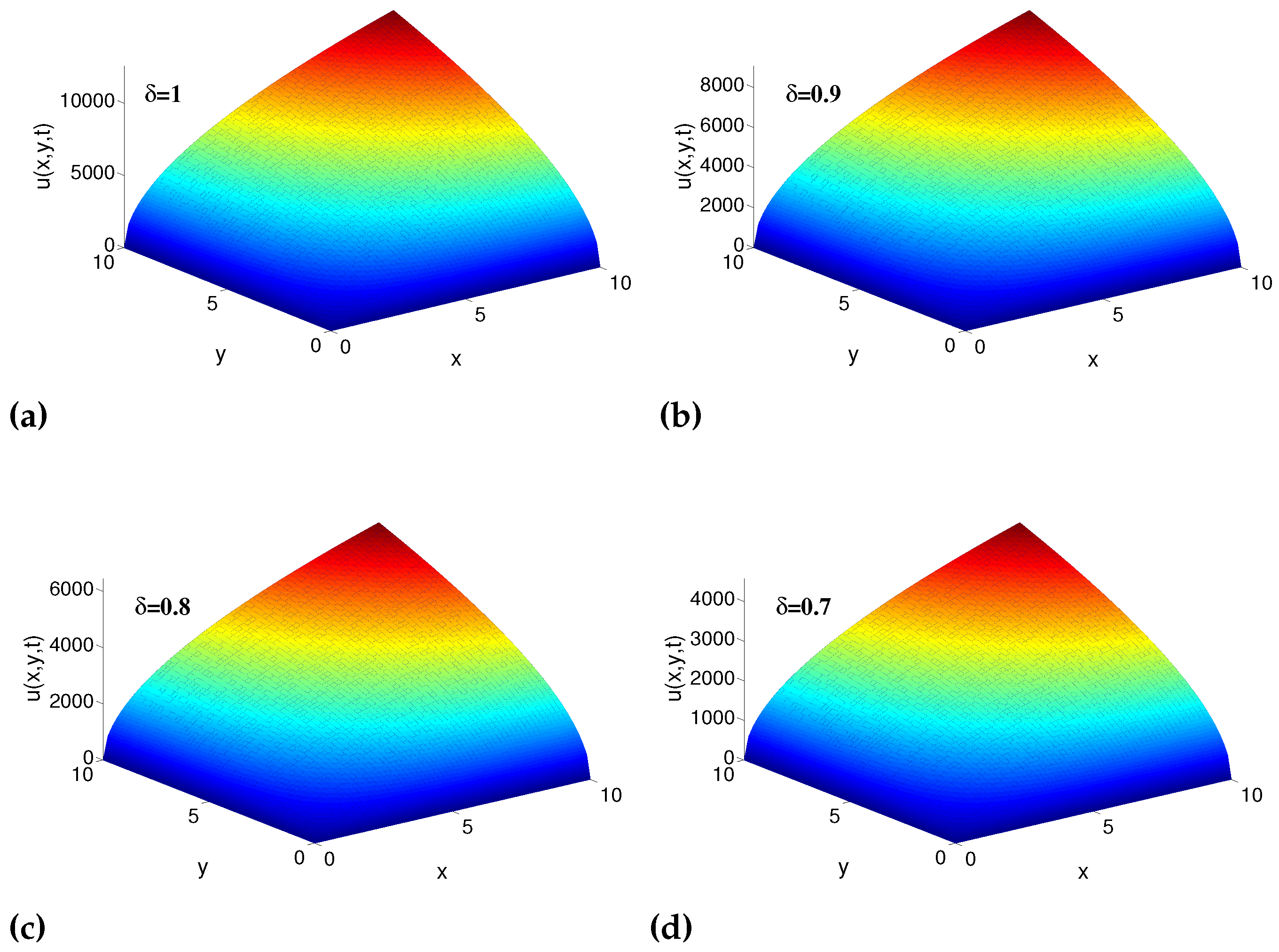
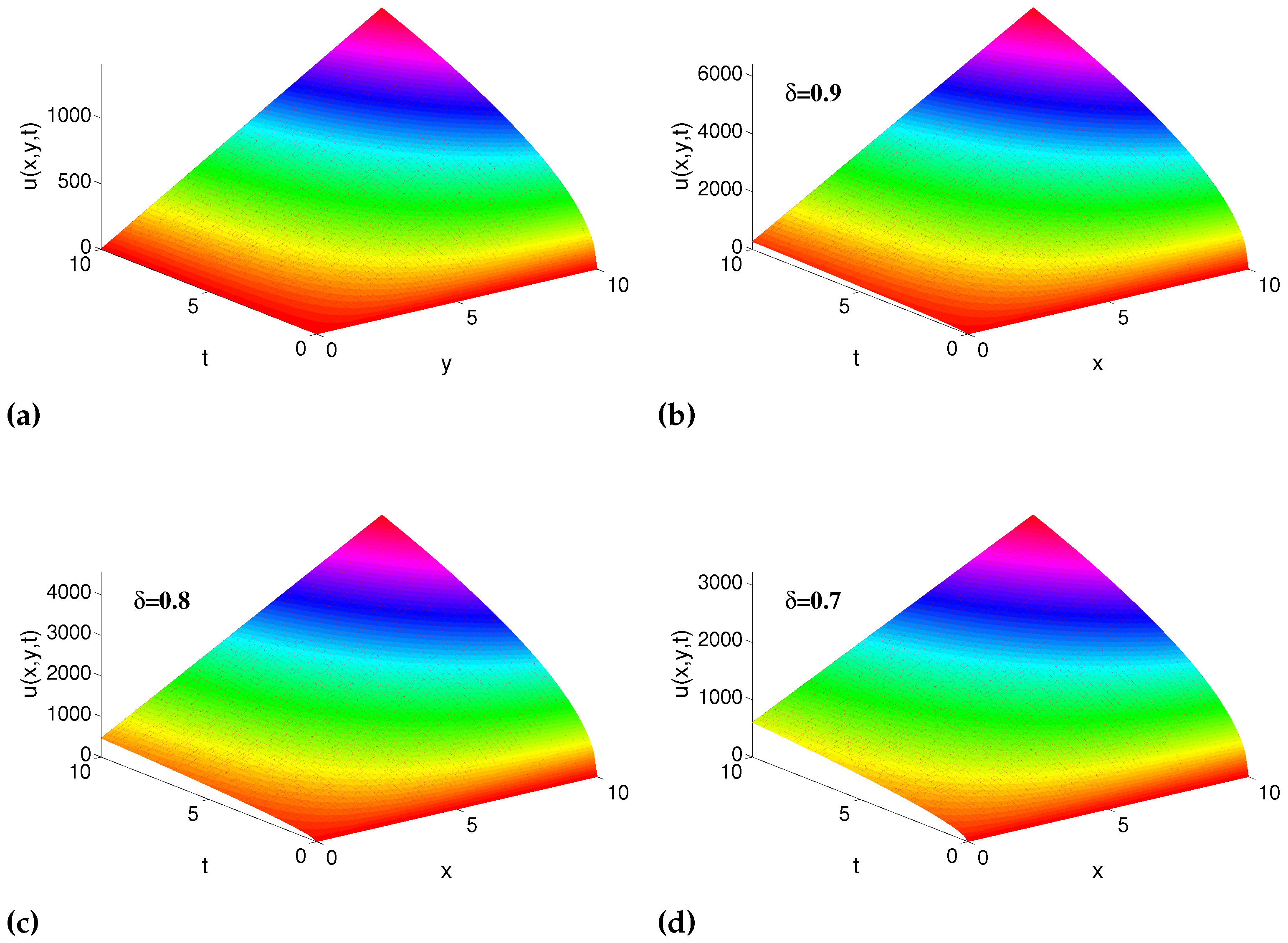
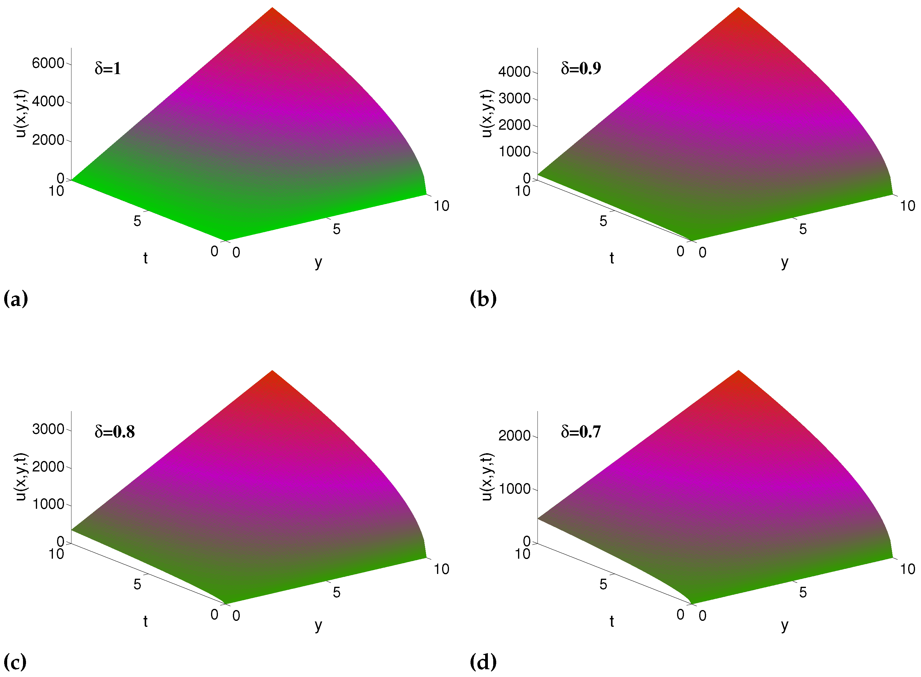
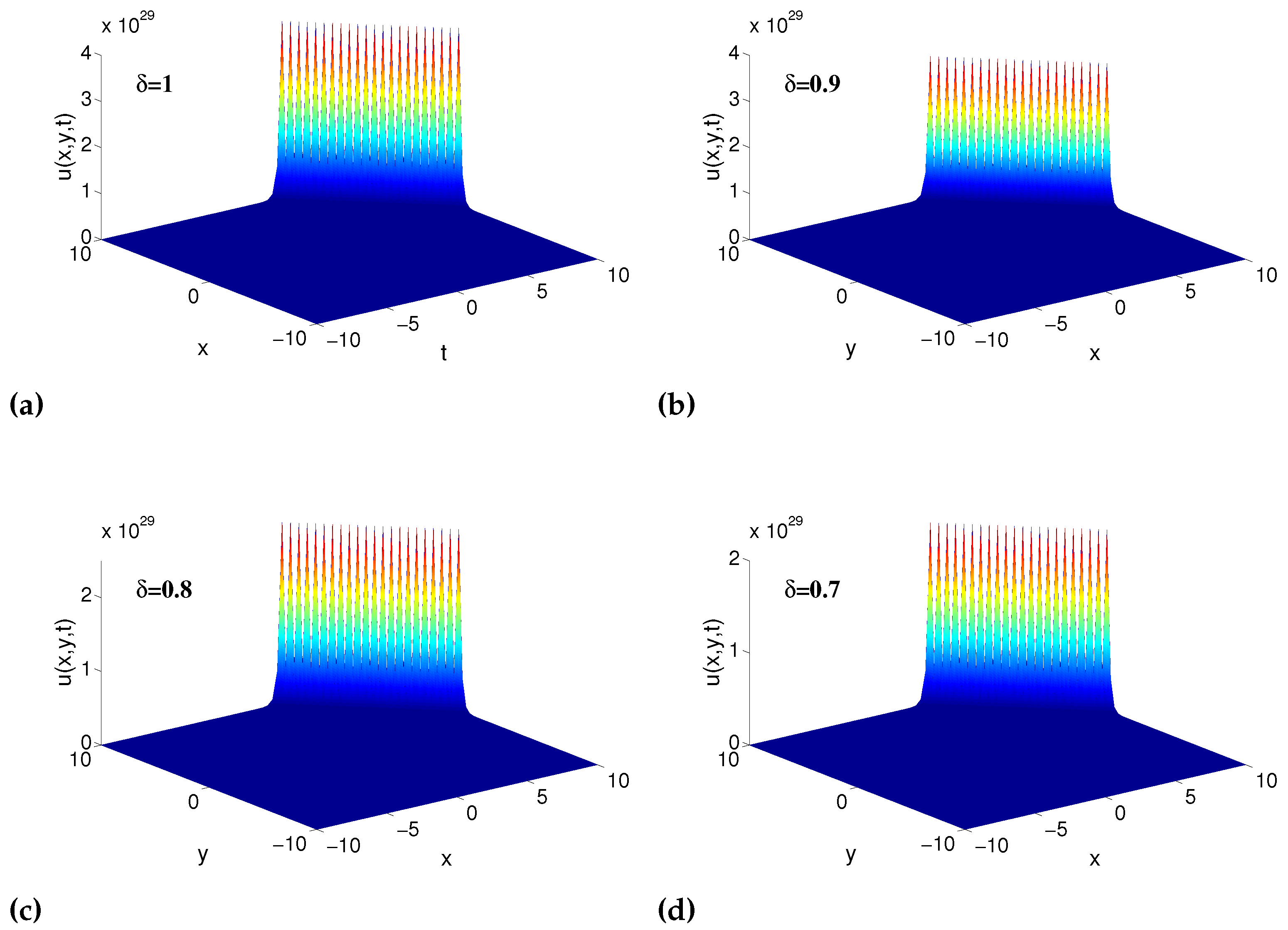
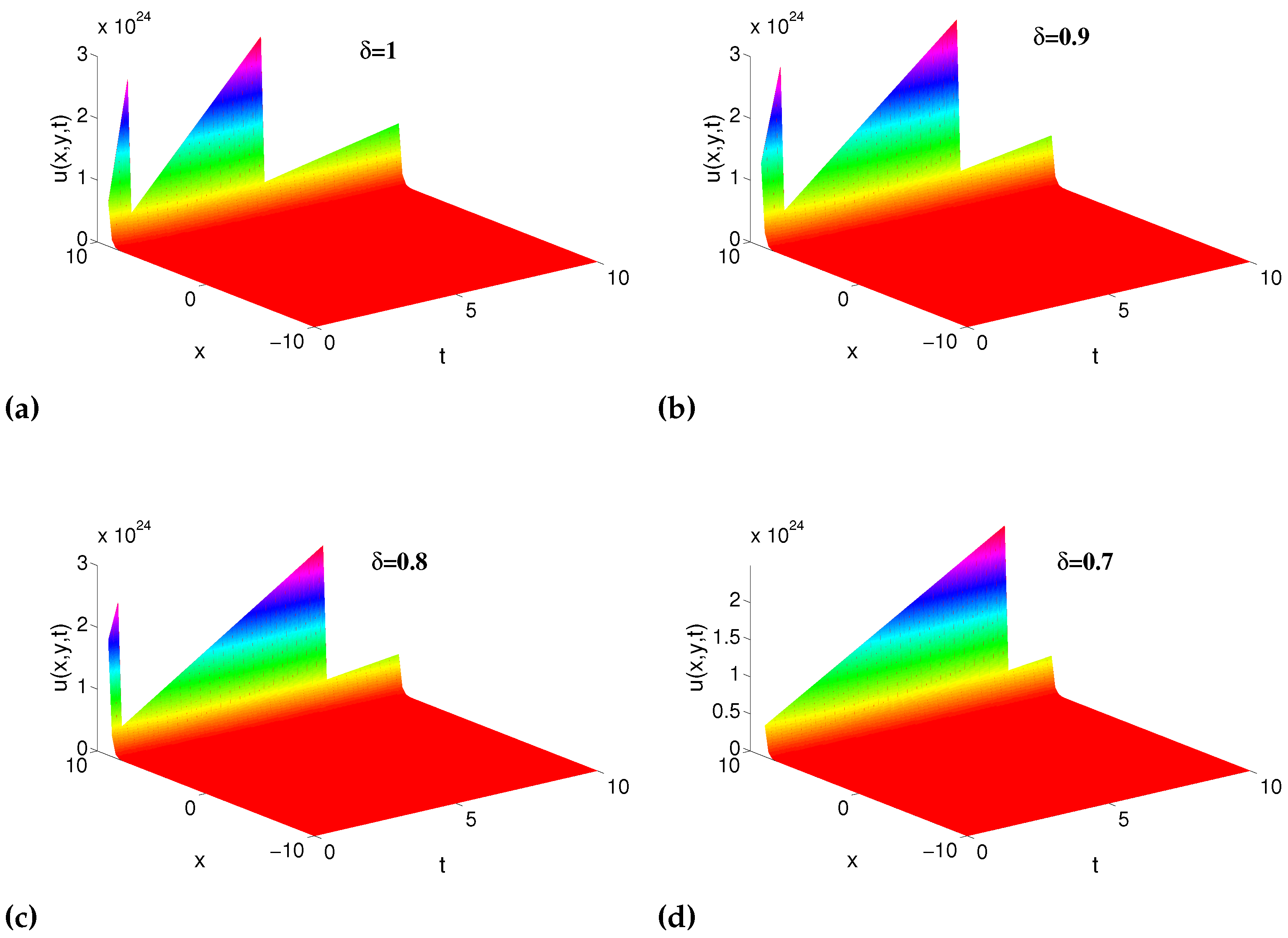
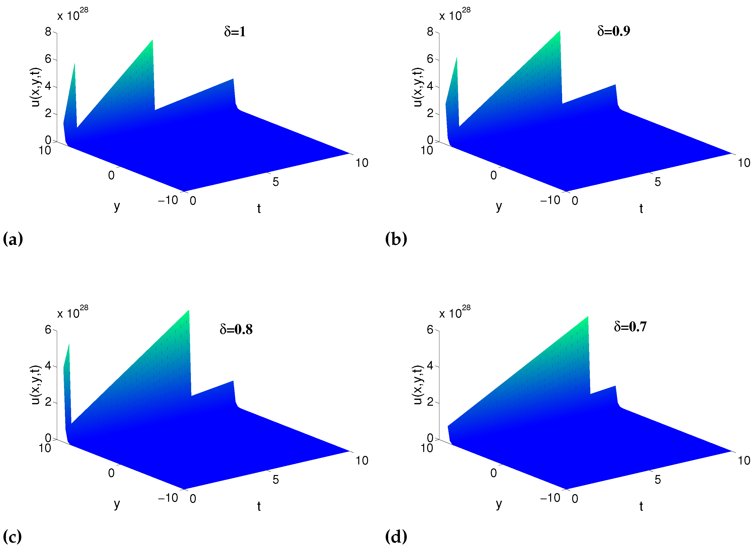
6.1. Numerical Plots and Comparison Tables

In this section, we present the numerical illustrations of the approximate solutions Equations (10) and (12) of the iterative examples considered on proposed model. For the graphical representations we consider the parameters as k = 3 , r = 50 and the fractional orders are considered to be ξ = 1 , 0.9 , 0.8 and 0.7. In each of the following figures the fractional orders are considered as Figure 1a–d. Figure 1 and Figure 2 shows the dynamics of the analytical approximate solution Equation (10). Similarly, Figure 3 depicts the dynamics in the behaviors of the solutions Equations (10) and (12) with x = 3 and x = 4 respectively and varying y , t . Furthermore, Figure 4 represents the changes that occur in the behaviors of the solutions Equation (12) respectively with t = 10 and varying the variables x , y . Here we see that when fractional order is large then the population density is also large, on the other hand population density decreases with the decrease in the fractional order.
Figure 5 shows the dynamical behavior of the solution Equation (12) with fixed y = 4 and y = 2 , respectively, and varying the other variables x , t . Furthermore, Figure 3 and Figure 6 depicts the dynamics in the behaviors of the solutions Equations (10) and (12) with x = 3 and x = 4 , respectively, and varying y , t . We observed that the considered scheme is rapidly convergent and is highly accurate.
It is observed that at lower fractional orders, the population density decreases, as can be seen in the figure. The considered operator shows an astonishing impact on the dynamics of the considered population model. The simulations show that the double Laplace transform is a powerful method that can be used to study such complexities with ease, without perturbing or dealing with the long-lasting polynomials.
Next, we present the comparison table between the exact and the approximate series solutions of the considered iterative examples in the sense of the C F operator. We considered k = 2 for Table 1, fractional-order as 1 and different values of variables x , y , t . Similarly, we supposed r = 50 for Table 2, fractional-order as 1 and various values of variables x , y , t . A good agreement is observed between the exact and approximate solutions which can be seen in the table.

7. Conclusions

In this manuscript, we proposed a fractional-order biological population system. Using fixed point theorems, we effectively developed proofs for the existence uniqueness of the considered model results. We obtained the numerical solutions of the fractional-order model (1) using DLADM. Furthermore, the convergence analysis of the proposed model with the considered method has been presented. From the numerical simulations, it is observed that when the fractional order is large then the population density is also large; on the other hand, population density decreases with the decrease in the fractional order. The error analysis shows that the technique approximate solution converges to the exact solution very quickly. As a result, we observed that the discussed methodology has significant advantages for obtaining analytical solutions for the FNDEs when compared to other methods. From the obtained results, we concluded that the DLADM is capable of reducing the volume of computational work as compared to other methods. The considered scheme does not need much analytical study and converges easily to the exact solution. In the future, we will suggest modifying the considered scheme of DLADM for the investigation of nonlinear partial differential equations and some advanced problems in fluid dynamics and elasticity dealing with integrals will be investigated in subsequent papers. Finally, we state that the considered method is indeed trustworthy and applicable to all nonlinear PDEs subject to initial condition.

Author Contributions

Conceptualization, M.u.R.; Data curation, F.S.A.-D.; Formal analysis, M.u.R. and A.A.; Funding acquisition, A.A. and F.S.A.-D.; Investigation, M.B.R.; Methodology, M.u.R. and M.B.R.; Resources, M.B.R.; Software, A.A.; Validation, M.u.R., M.B.R. and F.S.A.-D.; Visualization, F.S.A.-D.; Writing—original draft, M.u.R.; Writing—review & editing, M.B.R. All authors have read and agreed to the published version of the manuscript.

Funding

This research was funded by Taif University Researches Supporting Project number (TURSP-2020/326), Taif University, Taif, Saudi Arabia.

Institutional Review Board Statement

Not applicable.

Data Availability Statement

Not applicable.

Acknowledgments

The authors sincerely thank the reviewers for their constructive comments to improve the manuscript.

Conflicts of Interest

The authors declare that there is no conflict of interest.

References

  1. Gall, J.F. Brownian Motion and Partial Differential Equations Graduate Texts in Mathematics; Springer: Cham, Switzerland, 2016. [Google Scholar]
  2. Merwin, K. Analysis of a partial differential equation and real world applications regarding water flow in the state of Florida. McNair Sch. Res. J. 2014, 1, 8. [Google Scholar]
  3. Oldham, K.B.; Spanier, J. The Fractional Calculus; Academic Press: New York, NY, USA, 1974. [Google Scholar]
  4. Podlubny, I. Fractional Differential Equations; Academic Press: San Diego, CA, USA; New York, NY, USA; London, UK, 1999. [Google Scholar]
  5. Hilfer, R. Application of Fractional Calculus in Physics; World Scientific: Singapore, 2000. [Google Scholar]
  6. Zaslavsky, G.M. Hamiltonian Chaos and Fractional Dynamics; Oxford University Press: Oxford, UK, 2005. [Google Scholar]
  7. Magin, R.L. Fractional Calculus in Bio-Engineering; Begell House Publisher, Inc.: Connecticut, CT, USA, 2006. [Google Scholar]
  8. Debnath, L. Recent applications of fractional calculus to science and engineering. Int. J. Math. Math. Sci. 2003, 2003, 3413–3442. [Google Scholar] [CrossRef]
  9. Caputo, M.; Fabrizio, M. A new defi nition of fractional derivative without singular kernel. Prog. Fract. Differ. Appl. 2015, 1, 73–85. [Google Scholar]
  10. Atangana, A.; Baleanu, D. New fractional derivatives with nonlocal and non-singular kernel; Theory and application to heat transfer model. Therm. Sci. 2016, 20, 763–769. [Google Scholar] [CrossRef]
  11. Baleanu, D.; Fernandez, A.; Akgul, A. On a fractional operator combining proportional and classical differ-integrals. Mathematics 2020, 8, 360. [Google Scholar] [CrossRef]
  12. Kucche, K.D.; Sutar, S.T. Analysis of nonlinear fractional differential equations involving Atangana-Baleanu-Caputo Derivative. Chaos Solitons Fract. 2021, 143, 1–17. [Google Scholar] [CrossRef]
  13. Aydogan, S.; Baleanu, D.; Mousalou, A.; Rezapour, S. On approximate solutions for two higher order Caputo–Fabrizio fractional integro-differential equtions. Adv. Differ. Equ. 2017, 2017, 221. [Google Scholar] [CrossRef]
  14. Baleanu, D.; Mousalou, A.; Rezapour, S. On the existence of solutions for some infinite coefficient-symmetric Caputo–Fabrizio fractional integro-differential equations. Bound. Value Probl. 2017, 2017, 145. [Google Scholar] [CrossRef]
  15. El-Sayed, A.M.A.; Rida, S.Z.; Arafa, A.A.M. Exact solutions of fractional-order biological population model. Commun. Theor. Phys. 2009, 52, 992–996. [Google Scholar] [CrossRef]
  16. Kumar, D.; Singh, J.; Sushila, R. Application of homotopy analysis method to fractional biological population model. Rom. Rep. Phys. 2013, 65, 63–75. [Google Scholar]
  17. Ahmad, S.; Ullah, A.; Partohaghighi, M.; Saifullah, S.; Akgúl, A.; Jarad, F. Oscillatory and complex behaviour of Caputo-Fabrizio fractional order HIV-1 infection model. AIMS Math. 2022, 7, 4778–4792. [Google Scholar] [CrossRef]
  18. Saifullah, S.; Ali, A.; Irfan, M.; Shah, K. Time-Fractional Klein–Gordon Equation with Solitary/Shock Waves Solutions. Math. Prob. Eng. 2021, 2021, 6858592. [Google Scholar] [CrossRef]
  19. Kaabar, M.K.A.; Martínez, F.; Gómez-Aguilar, J.F.; Ghanbari, B.; Kaplan, M.; Günerhan, H. New approximate analytical solutions for the nonlinear fractional Schrödinger equation with second-order spatio-temporal dispersion via double Laplace transform method. Math. Methods Appl. Sci. 2021, 44, 11138–11156. [Google Scholar] [CrossRef]
  20. Khan, A.; Khan, T.S.; Syam, M.I.; Khan, H. Analytical solutions of time-fractional wave equation by double Laplace transform method. Eur. Phys. J. Plus 2019, 134, 163. [Google Scholar] [CrossRef]
  21. Sneddon, I.N. The Use of Integral Transforms; Tata McGraw Hill Edition: New Delhi, India, 1974. [Google Scholar]
  22. Losada, J.; Nieto, J.J. Properties of a new fractional derivative without singular kernel. Prog. Fract. Differ. Appl. 2015, 1, 87–92. [Google Scholar]
  23. Gadain, H.E. Application of double laplace ecomposition method for solving singular one dimentionla system of hyperbolic equations. J. Nonlinear Sci. Appl. 2017, 10, 111–121. [Google Scholar] [CrossRef]
  24. Kaya, D.; Inan, I.E. A convergence analysis of the ADM and an application. Appl. Math. Comput. 2005, 161, 1015–1025. [Google Scholar] [CrossRef]
Figure 1. The numerical simulations of Equation (10) with (a) δ = 1 , k = 3 (b) δ = 0.9 , k = 3 (c) δ = 0.8 , k = 3 (d) δ = 0.7 , k = 3 and t = 10 .
Fractalfract 06 00446 g001
Figure 2. The numerical simulations of Equation (10) with (a) δ = 1 , k = 3 (b) δ = 0.9 , k = 3 (c) δ = 0.8 , k = 3 (d) δ = 0.7 , k = 3 and y = 4 .
Fractalfract 06 00446 g002
Figure 3. The numerical simulations of Equation (10) with (a) δ = 1 , k = 3 (b) δ = 0.9 , k = 3 (c) δ = 0.8 , k = 3 (d) δ = 0.7 , k = 3 and x = 3 .
Fractalfract 06 00446 g003
Figure 4. The numerical simulations of Equation (12) with (a) δ = 1 , r = 50 (b) δ = 0.9 , r = 50 (c) δ = 0.8 , r = 50 (d) δ = 0.7 , r = 50 and t = 10 .
Fractalfract 06 00446 g004
Figure 5. The numerical simulations of Equation (12) with (a) δ = 1 , r = 50 (b) δ = 0.9 , r = 50 (c) δ = 0.8 , r = 50 (d) δ = 0.7 , r = 50 and y = 2 .
Fractalfract 06 00446 g005
Figure 6. The numerical simulations of Equation (12) with (a) δ = 1 , r = 50 (b) δ = 0.9 , r = 50 (c) δ = 0.8 , r = 50 (d) δ = 0.7 , r = 50 and x = 4 .
Fractalfract 06 00446 g006
Table 1. Comparison table between the exact [15] and the approximate series solution Equation (10).
(x, y, t)ExactApproximateError
(1, 1, 0)11.0001 9.8000 × 10 5
(1, 1, 1)31310
(2, 1, 2)86.267086.2670 1.3859 × 10 4
(2, 2, 2)122121.9998 1.9600 × 10 4
(3, 2, 1)75.934275.93420
(5, 2, 0)3.16233.1626 3.0990 × 10 4
(3, 5, 1)120.0625120.06250
(7, 5, 3)538.3633538.36210.0012
(1, 3, 0)1.73211.7322 1.6974 × 10 4
(10, 10, 1)3103100
(10, 10, 0)1010.0010 9.8000 × 10 4
(9, 2, 3)386.0803386.0795 8.3156 × 10 4
(4, 4, 1)1241240
(4, 8, 4)684.4794684.47770.0017
(8, 9, 5) 1.2813 × 10 3 1.2813 × 10 3 0.0033
(9, 8, 1)263.0437263.04370
(0.5, 1, 1)21.920321.92030
(0.2, 1, 0)0.44720.4473 4.3827 × 10 5
(0.1, 0.1, 0)0.10000.1000 9.8000 × 10 6
Table 2. Comparison table between the exact [15] and the approximate series solution Equation (12).
(x, y, t)ExactApproximateError
(−10,−10, 0) 3.7201 × 10 44 3.7201 × 10 44 3.7201 × 10 52
(−10, −10, 1) 1.8600 × 10 43 1.8600 × 10 43 0
(−6, −6, 0) 8.7565 × 10 27 8.7565 × 10 27 8.7565 × 10 35
(−6, −6, 1) 4.3783 × 10 26 4.3783 × 10 26 0
(0, −2, 2) 3.1780 × 10 4 3.1780 × 10 4 1.3620 × 10 12
(0, 2, 2) 1.9824 × 10 5 1.9824 × 10 5 2.2026 × 10 4
(−10, 0, 10) 7.9079 × 10 21 7.9079 × 10 21 1.7359 × 10 29
(−10, 1, 10) 1.1736 × 10 18 1.1736 × 10 18 2.5763 × 10 27
(−8, 0, 8) 1.4020 × 10 16 1.4020 × 10 16 2.9738 × 10 25
(8, 1, 8) 2.0807 × 10 14 2.0807 × 10 14 4.4136 × 10 23
(−2, 0, 2) 4.0860 × 10 4 4.0860 × 10 4 4.4948 × 10 6
(2, 0, 2)0.06060.0600 6.6709 × 10 4
(−1, −1, 0) 4.5400 × 10 5 4.5400 × 10 5 4.4948 × 10 6
(1, 1, 1) 1.1013 × 10 5 1.1013 × 10 5 0
(2, −2, 0)11.09900.0990
(−3, −1, 2) 1.8550 × 10 8 1.8550 × 10 8 2.0406 × 10 10
(0, −2, 1) 2.2700 × 10 4 2.2700 × 10 4 0
(2, 0, 0) 4.5400 × 10 5 4.5400 × 10 5 4.4948 × 10 6
Publisher’s Note: MDPI stays neutral with regard to jurisdictional claims in published maps and institutional affiliations.

