Article

Minkowski’s Loop Fractal Antenna Dedicated to Sixth Generation (6G) Communication

by
Maria-Alexandra Paun
1,2,
Mihai-Virgil Nichita
3,
Vladimir-Alexandru Paun
4 and
Viorel-Puiu Paun
5,6,*
1
School of Engineering, Swiss Federal Institute of Technology (EPFL), 1015 Lausanne, Switzerland
2
Division Radio Monitoring and Equipment, Section Market Access and Conformity, Federal Office of Communications OFCOM, 2501 Bienne, Switzerland
3
Doctoral School, Faculty of Applied Sciences, University Politehnica of Bucharest, 060042 Bucharest, Romania
4
Five Rescue Research Laboratory, 75004 Paris, France
5
Department of Physics, Faculty of Applied Sciences, University Politehnica of Bucharest, 060042 Bucharest, Romania
6
Academy of Romanian Scientists, 050094 Bucharest, Romania
*
Author to whom correspondence should be addressed.
Fractal Fract. 2022, 6(7), 402; https://doi.org/10.3390/fractalfract6070402
Submission received: 24 June 2022 / Revised: 17 July 2022 / Accepted: 19 July 2022 / Published: 21 July 2022

Abstract

:
In this study, we will discuss the engineering construction of a special sixth generation (6G) antenna, based on the fractal called Minkowski’s loop. The antenna has the shape of this known fractal, set at four iterations, to obtain maximum performance. The frequency bands for which this 6G fractal antenna was designed in the current paper are 170 GHz to 260 GHz (WR-4) and 110 GHz to 170 GHz (WR-6), respectively. The three resonant frequencies, optimally used, are equal to 140 GHz (WR-6) for the first, 182 GHz (WR-4) for the second and 191 GHz (WR-4) for the third. For these frequencies the electromagnetic behaviors of fractal antennas and their graphical representations are highlighted.

1. Introduction

The commencement history of the 6G activity is quite recent in time. In the USA, the Federal Communications Commission (FCC) has thus begun to provide tentative 6G frequency band licenses, starting with the year 2019. By its statute, the FCC organization will offer innovative engineers a minimum ten-year authorization to test the established frequency spectrum of new sixth generation industrial objects and utilities. As for the appointment with the appellative 6G, this is the abbreviation of the new generation, in fact the sixth era of wireless networks, declared as the descendant of 5G technics. Ultimately, as a successor to previous generations, the new 6G generation is expected to amplify the existing qualities of the 5G generation.
This study of the subject in question is ready to host excellent information, such as 6G radio-frequency domain, and frequency bands and ultimately expose 6G technics [1,2,3]. In short, the frequency spectral range, falling in the 95 GHz (gigahertz) to 3 THz (terahertz) domain, will be experimentally initiated for utilization to allow technicians reverie of the next radio-wireless descendent and outset new activity. However, it is self-evident that the frequency band being considered superfluous to the original purpose could deliver an extra rapid Internet exploitation for ascensive data practice, such as extra determination computer imaging and sensing signal appliances.
First, we talk about what 6G is, how it is possible to achieve 6G communications (about frequencies, especially) and how current this requirement is. One of the potential purposes of it is to substitute or operate together with those known as 5G networks and be superior to them [4]! Moreover, as the first major advantage, it can be stated that it can afford meaningfully more dynamic propagation, at a signal velocity of approximately 95 Gbit/s, taken as the reference speed in our case. Thus, in the distributed communications area, the so-called 6G is evidently the sixth engendering standard for wireless transmission technics in radio natural networks (see frequency bands used).
The present paper is organized by comprising the six following chapters/sections. In Section 1, the first work section, a brief general introduction is presented. After the introductory remarks, in Section 2, the essential notions about fractal geometry are mentioned, with the specification of some Minkowski fractal characteristics. In Section 3, a review of the Minkowski fractal antenna designs inspired by mutual fractal patterns is made. In Section 4, the impact of performances in the utilization of fractal antenna are reported. At this point, important results such as the charge and current distribution of fractal island antenna, electric and magnetic fields 3D distribution, Minkowski fractal antenna pattern radiation and overlay, signal magnitude versus frequency for Minkowski fractal antenna, impedance versus frequency as well as signal magnitude versus frequency for VSWR are obtained and discussed. In Section 5, a comparison of Horn antenna versus Minkowski fractal antenna, mostly among operating parameters, is highlighted. At the end, in Section 6, the last work section, the conclusions of this study are drawn.

2. Fractal Antennas, Fractals Geometry, Minkowski Fractal Characteristics

2.1. About the Fractal Antennas

From the beginning, we can say that the fractals idea has motivated the electrical engineering collectivity to do a thorough investigation about the fact that the fractal geometries could serve in employment at the special antennas design, subsequently named fractal antennas. Thus, in this sense, our work is intending now to highlight the involvement of fractals in fractal antenna technology. The novel research pursuit has as a result obtained extremely spectacular miniature devices, of great perspective, considered basic bricks in the development of professional antennas.
The fractal type antenna has applications in the military area, in particular, as well as the economical-commercial zone, wherein by projecting the device, it controls its advisable ownerships, such as:
  • Compact/short dimension;
  • Reduced perimeter;
  • Multi-band frequency;
  • Conformal typology.
Some fractal type antenna shortcomings are the following:
  • Antenna gain losing;
  • Complicated composition;
  • Smaller benefits in dimension according to early recurrence.
Fractal antennas are welcome to be studied as being able to support frequencies in the 6G spectrum, obviously after determining the corresponding fractal geometric shape and the iteration required for the established frequency.

The 6G Radio Frequency

The frequency bands for which this 6G antenna was designed are presented in Table 1 [5].
Among the bidder fractal objects, the most popular are fractal curves such as the fractal curve type, for example, the Koch Curve (1.2618), Sierpinski Triangle (1.5848), Sierpinski Carpet (1.8928), Koch Snowflake (1.2618) and Minkowski Curve (1.465), with fractal dimensions written in parentheses. For this study, we found that the Minkowski Curve meets our requirements [6], more precisely Minkowski’s loop, which is justified to do this research.

2.2. About the Fractal Character: Minkowski’s Loop

This section introduces a few considerations about the fractal character of the Minkowski’s loop and Minkowski fractal antenna. Let us briefly discuss the effects of using the Minkowski fractal figure on each side of the square area antenna in certain recurrences, through which to find its ideal shape, to be used in the design of the corresponding fractal antenna. First of all, we are interested in how the fractal shape is realized from a geometric point of view and the iterative process that is necessary to obtain the fractal figure considered ideal for the proposed purpose [7].
Currently, by employing the Minkowski procedure, this can be resumed, and the n-th reiteration is accomplished by sharing a linear section an−1 into five subsections rncnbncnrn and repeating it over and over again. Between the values of the five segments is the following constitutive relation an−1 = 2rn + bn, in which cn is the fractal deep of the generator in the n-th Minkowski recurrent relation (we start from a straight line, and we obtain the step generator, height/indentation equal to rn), Figure 1, baseline. Another indicator used, named δ n , is the iteration factor in the respective iteration and is noted as δ n = C n / B n . Both values of equality, respectively Cn and δ n at the n-th iteration, are adaptable and will be optimized based on the design performances of the developed antenna.
The measure D of fractal characteristics can be decided by a logarithmic rapport. The general equation is s = pD, a power type law, as in the calculus formula for D
s = p D ,   log s = l o g p D = D l o g p ,   D = l o g s l o g p = l n s l n p
where s is the number of self-similar segments obtained from one portion after every repetition and p is the number of parts obtained from one segment of every repetition [7,8].
Conformable to Formula (1), the computed fractal measure, named fractal dimension, is equal to 1.465 [7]. The fractal dimension D of a fractal curve is an indication of superior achievement of space-addition (or filling) for the fractal in cause [9]. Yet, some fractal curves cannot be utilized in the fractal antenna design practice. However, several fractal geometries have been successfully employed in the projection of different antennas.
In Figure 1a–c, the steps of growth of the modified Minkowski fractal structure are shown, respectively, as (a) the square ring, (b) the 1st iteration and (c) the 2nd iteration. In Figure 1d, the first three iterations of Minkowski’s loop are introduced, together with the linear generator consisting of five segments. More precisely, in the outline above, we start from the initial appearance (one single figure), named the Minkowski initiator and arrive through three iterations to the fourth complex figure (last figure). This is the fractal figure used in making the fractal antenna in our study.
Suitable to Falconer [10], the amended variant of the Minkowski fractal geometry is called multi-fractal or fractal geometry with above one ratio in the generator, such as a1 and a2. In this situation, the fractal dimension, D, can be achieved, as in the solution of the next equation:
2 ( 1 a 1 2 ) D + 2 a 2 D + a 1 D = 1
where a1 = L1/Lo, respectively, a2 = L2/Lo, Figure 1b.
In Figure 2, the variation of the fractal dimensions D of the modified Minkowski fractal, with the a1 = x (on ox axis) and a2 = y (on oy axis) functioning as independent variables is presented. The value of D is greater than 1 and less than 2 (in our chart less than 1.99, to be exact).

3. Minkowski Fractal Antenna

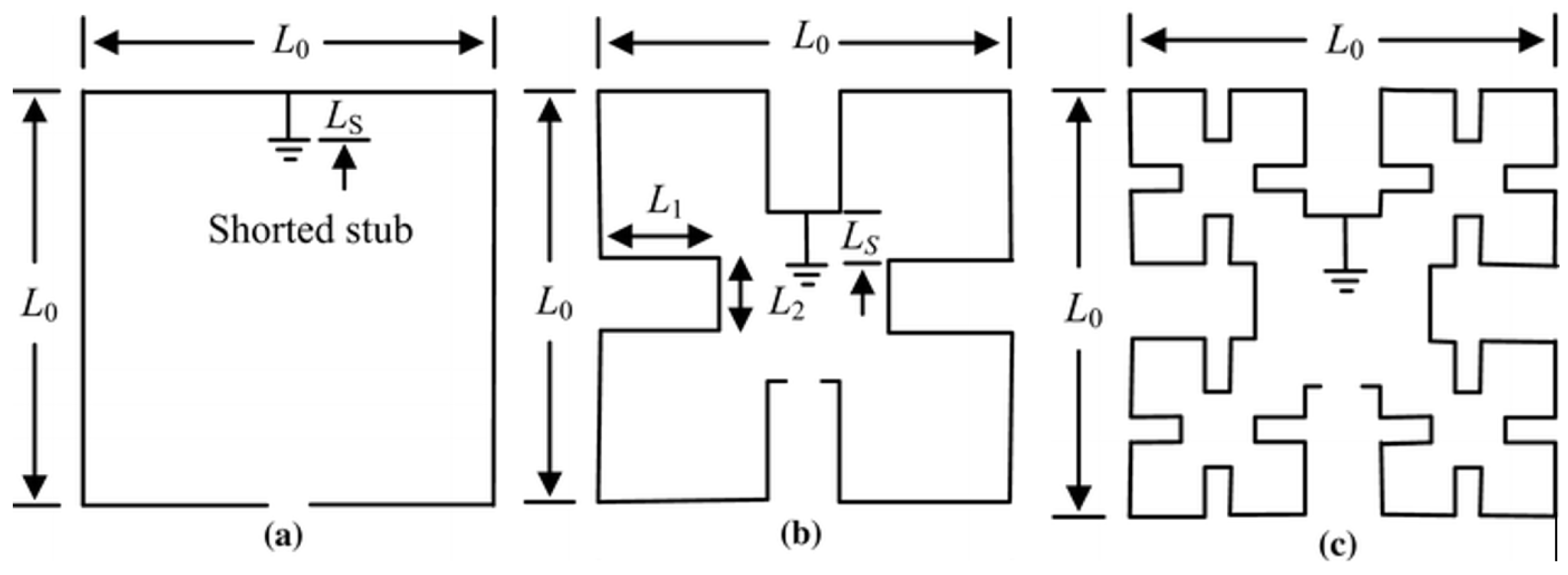
The fractal island object named the Minkowski’s loop geometric figure was used to develop a fractal type antenna, more precisely to make a professional antenna. As is known, the fractal antenna is the profitable beneficiary of a self-similarity project able to increase to the maximum lengthiness, to grow the contour of a physical entity, which emits electromagnetic waves in space, or to be in receipt of electromagnetic waves within a circumscribed area, or rather into a surface, respectively volume restricted [11]. The chosen fractal antenna has the shape of a “Minkowski’s loop”, with four iterations placed above a ground plane antenna (electrical conductance area) [12].
For printed circuit boards, a ground plane is a large area of copper foil on the board, which is connected to the ground terminal of the power supply and serves as a return path for the current from various components on the board; therefore, it seems the most appropriate definition [13].
In Figure 3, the antenna corresponding to the drawn fractal is graphically described. The power supply/current alimentation to the antennas is normal [9]. For the template in the figure above, there have been set in the simulation environment titled Antenna Designer offered by MATLAB R2021a, the following values:
  • Length = 0.03 m; Width = 0.028 m; StripLineWidth = 0.0008 m; SlotLength = 0.004 m;
  • SlotWidth = 0.00585 m; Height = 0.001 m; GroundPlaneLength = 0.05 m;
  • GroundPlaneWidth = 0.03 m; FractalCenterOffset (m) = [0 0]; Tilt (deg) = 0; TiltAxis = [1 0 0].
The dielectric used is air, with a value of relative dielectric permittivity εr (air) =1 and which is present in a layer of 0.00004 m. The absolute dielectric permittivity of the classical vacuum is ε0 = 8.8541 × 10⁻¹² F⋅m−1.
The favorable frequency bands for which this 6G Minkowski fractal antenna (four iterations) was here designed, are 110 GHz to 170 GHz (WR-6), respectively, 170 GHz to 260 GHz (WR-4) [5]. The strips were chosen according to the indications on the website https://www.miwv.com/what-is-6g (accessed on 11 June 2022).

The Revised Minkowski Geometry Figure of Fractal

The particular standard used in the fractal figure choice, as far as that goes in the radiation circuit of minimum measure, is without question its size. With the increase in the fractal size, the fractal figure replenishes the suitable domain much better than usual. To achieve the antenna able to work in the planned frequency range, we benefit from the Minkowski type fractal decomposition scheme to the quadratic area, first of all for the enlargement of lengthiness of the actual effluent route and thereby diminution of the device physical dimension. The fundamental Minkowski type fractal item, presented in detail in Figure 3, is utilized for the enhancement of the actual running lengthiness, named to be the depth of the fractal. The Minkowski type fractal item can be included into the composition as a structure one after the other, added to every part developed of the Minkowski fractal process, at a precedent recurrence step. In this way, it is the obtained/realized enlargement of actual route lengthiness, and it minimized the antenna dimension for a certain frequency of resonance.

4. Results and Discussion

Antenna sketch and project are generally easy to accomplish, but all component parts, which are incorporated in the final project, are frequently the more exciting ones.
By definition, the so-called antennas as parts of a circuit deal with the reception or transmission of electromagnetic waves in the environment. In this context, project managers are concerned with priority in obtaining appropriate performances, especially for the gain, and in the directivity of the designed antennas.
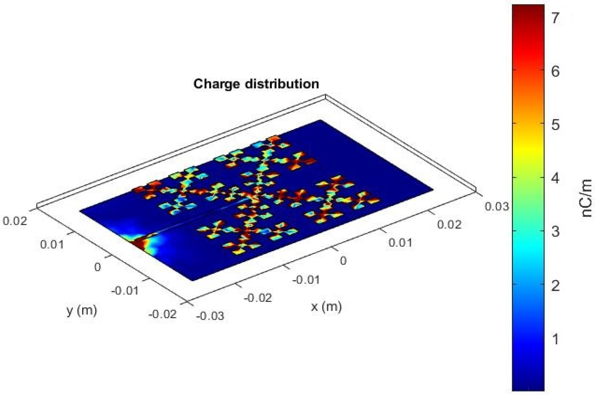
Thus, we will continue to speak about the radiation patterns, power gain and power dissipation of a fractal Minkowski antenna, completed on this occasion. The charge distribution simulation (Figure 4), and respectively the current distribution simulation (Figure 5) of fractal island antenna, are made only for the resonance frequency equal to 140 GHz, (WR-6). In Figure 6 and Figure 7, the antennas corresponding to the drawn fractal are graphically described. The power supply/current alimentation to the antennas is normal (Figure 3 and Figure 4), and in Figure 6 and Figure 7, is lateral.
Two more interesting frequencies are discovered where the Minkowski fractal antenna resonates (182 GHz and 191 GHz), (WR-4).
In Figure 8 and Figure 9, current distribution simulations of fractal island antenna are made only for the resonance frequencies equal to 182 GHz and 191 GHz, respectively. Power supply/current bias to the antennas is normally made in the figure on the left, and in the figure on the right, is laterally made!
In Figure 10, the Azimuth pattern of the Minkowski fractal antenna, respectively signal directivity, at 140 GHz resonance frequency, is presented. In Figure 11 are graphically represented the Electric (blue) and Magnetic (red) Fields 3D Distribution, for normally powered antenna [14]. It is a sphere uniformly distributed with the vectors of the two fields, E and H, but with a higher density in the area of the two geographical poles. In the left corner of the sketch is the Minkowski flat fractal antenna, designed for the fourth iteration.
Figure 12 and Figure 13 are figures with 3D (spatial) representation. These are made to indicate the behavior of the Minkowski fractal antenna pattern radiation, having a colored band on the right, graded in dBi. Unlike the known units named dB (decibels), the dBi (isotropic decibels) units, they are also decibels, but in relation to an isotropic radiator device.
Figure 14 presents impedance versus frequency, in two distinct curves. The first curve is resistance (blue) and the second is reactance (red). These are almost horizontal variations curves, except for the end-of-scale effects [15].
Figure 15 shows the signal magnitude (dB) versus frequency (GHz) (blue line) for the Minkowski fractal antenna, where the last listed refers to the Voltage Standing Wave Ratio (VSWR) [16].
Such that a radio device (which emits or receives electromagnetic waves) must be able to provide energy to its antenna, the radio total impedance and emission circuits line impedance must be well tuned according to the antenna’s effective resistance. The impedance is thus the actual resistance of an integral electric circuit or the constituent in an alternative current, which results from both ohmic resistance and reactance mixed effects [16,17]. The parameter Voltage Standing Wave Ratio (VSWR) is the physical degree that numerically depicts how well the antenna is coupled to the impedance provided of the radio line or emission line to which it is related. The VSWR is a service of the numerical reflection factor, which describes the energy reflected from the device used to transmit or receive electromagnetic signals.
In Figure 16, Figure 17 and Figure 18 of the Minkowski fractal antenna for two, three, and respectively, four iterations, the self-reflection coefficient S11 and return loss graphics are presented.
Figure 16, Figure 17 and Figure 18 show the graphs for (a) the self-reflection coefficient (S11), and respectively, the return loss for (b), of the Minkowski type fractal antennas for two, three and four iterations.
Now, it can be said that S-parameters sometimes get used interchangeably with the return loss, insertion loss and reflection coefficient, and often without discernment. In particular, there seems to be the casual strong confusion around the dissimilarity between the return loss versus the reflection coefficient, as well as because these associate to (S11). These mistaking overlaps do occur, however, from the fact that these quantities defined above all describe the reflection of a wave propagating from a reference pack, either that it is a terminal transmission line or that it is a grid of preset circuits, ultimately.

Fractal Antenna Measurements

According to a number of relevant simulations and measurements on Minkowski’s loop-based fractal configurations, the optimum one is presented in the following figure. In such an iterative procedure, an initial structure is replicated countless times at different scales, positions and directions, to obtain the final fractal structure. In Figure 19, the photography of a fabricated antenna from a fractal curve scheme of the Minkowski’s loop third iteration can be noted.
The modeling and design process of the antenna are completed in MATLAB with the help of the AntennaDesigner toolbox: (https://www.mathworks.com/help/antenna/ref/antennadesigner-app.html (accessed on 11 June 2022)). The toolbox first asks for the frequency for which one wants to design the antenna. Once this value is entered, a prototype is made which can then be adjusted until the simulations suit the designer. We modify certain dimensions of the fractal until we obtain the desired values for impedance, VSWR, etc. All graphs are obtained with this program. The iterative process is performed up to the third iteration. The Rogers 4350 0.8 mm thick material is used for the dielectric having the relative permittivity of εr = 4.4. The fractal antenna is fed from the normal position by coaxial cable having the inner and outer diameters of the SMA connector. The scale factor of antennas is 1/3 and the stage of iteration is n = 3. The size of the substrate and the patch are the same. At the end of the modeling, the Gerber files are generated, useful for printing the antenna wiring on the dielectric material (the PCB design has to be completed with a specialized device to strictly observe the fractal dimensions). In the measurements effectuated with the fractal antenna obtained, the VDI - Erickson Power Meters (PM5B) were used. This power meter, covering both analog and digital carriers, is a calibrated calorimeter-style power meter for 75 GHz to >3 THz applications. It offers power measurement ranges from 1 µW up to 200 mW. The PM5B is the de facto standard for frequency > 100 GHz power measurement and can be used in measurements such as VSWR for antenna and cable, antenna return loss and cable return loss to measure forward power and measure reflected power.
From the investigation of the graph representations, a good match of the experimental results with the simulated ones is observed. An excellent overlap, between simulated and measured impedance, is presented in Figure 20. The graph in Figure 21 shows that we have low, reduced VSWR values. This is gratifying, because the lower the VSWR, the better the antenna is impedance-matched to the transmission line and the higher the power delivered to the antenna. Furthermore, a small VSWR reduces reflections from the antenna.

5. Horn Antenna versus Minkowski Fractal Antenna

The Minkowski fractal antenna and the classic Horn antenna were discussed, for example [14]. In both representations, the constituent elements of the antennas in the plates present in the perpendicular plane y0z (black drawing on an olive background) are passed, generically called the anisotropic fractal meta-surface and, respectively, the dual-band printed Horn antenna.
Figure 22 shows two distinct antennas operating in the same frequency band specific to the 6G communications frame, in order to make a direct comparison of the quality of the emission factors. From our assumptions, this concept is among primal designs for a meta-surface applied to a dual-band antenna with contrary beams. In a positive vision, the proposed meta-surface-based fractal antenna concept may present novel opportunities in the projection of multi-functional antennas [18].
As can be seen from the graphical representations, the Minkowski’s loop fractal antenna is better in terms of pattern radiation overlay, having the signal strength close to 10 dBi (after the dark red color that appears in the figure on the left), being present on a larger surface such as emissivity [15].
Regarding the directivity and gain of the two compared types of antennas, we present two graphs in Figure 23 and Figure 24, both at the resonant frequency of 140 GHz. The gains are different from each other, with values of 14.63 dB for the Horn antenna and 3.133 dB for the Minkowski fractal antenna, the fourth iteration. Figure 23 and Figure 24 highlight the directivity qualities and the gain associated to the individual antenna, graphically represented in 2D, each separately [16]. Thus, we have the main directivity θ = 295° at a gain G = 3.13 dB for the fractal Minkowski antenna, and a main directivity θ = 270° at a gain G = 14.6 dB for the Horn antenna.
Finally, we mention that in the graphical representations proposed in this paper we used the software programs initiated in Image Clustering Algorithms to Identify Complicated Cerebral Diseases, in a medical article [19].

6. Conclusions

In this paper, the engineering construction of a special Sixth Generation (6G) antenna has been presented, based on the fractal geometry called Minkowski’s loop. The antenna has the shape of this known fractal, set finally at four iterations, to obtain a maximum electromagnetic performance.
The frequency bands for which this 6G fractal antenna was projected in the article are 170 GHz to 260 GHz (WR-4), and 110 GHz to 170 GHz (WR-6), respectively. The three resonant frequencies, optimally used, are equal to 140 GHz (WR-6) for the first, 182 GHz (WR-4) for the second and 191 GHz (WR-4) for the third. For these frequencies, the electromagnetic behaviors of fractal antennas are well shown.
Our review highlighted qualities of fractal geometry in the antenna’s design, made a classical analysis of the Minkowski fractal antenna, and calculated and graphically represented the electric and magnetic parameters such as charge and current distribution, electric and magnetic fields 3D distribution, impedance, radiation efficiency, Azimuth pattern and directivity, radiation pattern and VSWR.
It is immediately noticeable that, as with most fractal antennae, the radiation pattern, and consequently, the detection efficiency and quality of the emission factors, do not fluctuate umpteen with respect to frequency, mathematically speaking.
The antenna gain is reasonable compared to other fractal antennas, namely, we have a gain equal to G = 3.13 dB at an angle of main directivity equal to θ = 295°, for the fractal Minkowski’s loop antenna (the three iterations). A good match of the experimental results with the simulated ones is observed.

Author Contributions

Conceptualization, V.-P.P. and M.-A.P.; methodology, V.-P.P.; software, M.-V.N. and V.-A.P.; validation, V.-P.P., M.-A.P. and V.-A.P.; formal analysis, V.-P.P., M.-A.P. and V.-A.P.; investigation, V.-A.P. and M.-A.P.; resources, V.-A.P. and M.-A.P.; data curation, M.-V.N. and V.-A.P.; writing—original draft preparation, V.-P.P.; writing—review and editing, M.-A.P. and V.-P.P.; visualization, V.-A.P. and M.-V.N.; supervision, V.-P.P.; project administration, V.-P.P. All authors have read and agreed to the published version of the manuscript.

Funding

This research received no external funding.

Institutional Review Board Statement

Not applicable.

Informed Consent Statement

Not applicable.

Data Availability Statement

The data used to support the findings of this study cannot be accessed due to commercial confidentiality.

Acknowledgments

The co-authors M.-A.P., V.-A.P. and V.-P.P. would like to thank Jenica Paun for her continuous kind support.

Conflicts of Interest

The authors declare no conflict of interest.

References

  1. Hajiyat, Z.; Ismail, A.; Sali, A.; Hamidon, M.N. Antenna in 6G Wireless Communication System: Specifications, Challenges, and Research Directions. Optik 2021, 231, 166415. [Google Scholar] [CrossRef]
  2. Sa’don, S.N.H.; Kamarudin, M.R.; Dahri, M.H.; Ashyap, A.Y.I.; Seman, F.C.; Abbasi, M.I.; Abidin, Z.Z. The Review and Analysis of Antenna for Sixth Generation (6G) Applications. In Proceedings of the 2020 IEEE International RF and Microwave Conference (RFM), Kuala Lumpur, Malaysia, 14–16 December 2020. [Google Scholar]
  3. Wu, Y.; Singh, S.; Taleb, T.; Roy, A.; Dhillon, H.S.; Kanagarathinam, M.R.; De, A. (Eds.) 6G mobile Wireless Networks; Springer: Cham, Switzerland, 2021. [Google Scholar]
  4. Nichita, M.V.; Paun, M.A.; Paun, V.A.; Paun, V.P. On the 5G Communications: Fractal-Shaped Antennas for PPDR Applications. Complexity 2021, 2021, 9451730. [Google Scholar] [CrossRef]
  5. Kato, Y.; Omori, K.; Sanada, A. D-Band Perfect Anomalous Reflectors for 6G Applications. IEEE Access 2021, 9, 157512–157521. [Google Scholar] [CrossRef]
  6. Prakriti, S. Application of Fractal Antennas with advantages and disadvantages. Int. J. Creat. Res. Thoughts 2018, 6, 551–554. [Google Scholar]
  7. Mandelbrot, B. Fractal Geometry of Nature; Freeman: New York, NY, USA, 1983; pp. 25–57. [Google Scholar]
  8. Paun, V.P.; Agop, M.; Chen, G.; Focsa, C. Fractal-Type Dynamical Behaviors of Complex Systems. Complexity 2018, 2018, 8029361. [Google Scholar] [CrossRef] [Green Version]
  9. Nichita, M.V.; Paun, M.A.; Paun, V.A.; Paun, V.P. Fractal Analysis of Brain Glial Cells. Fractal Dimension and Lacunarity. Univ. Politeh. Buchar. Sci. Bull.-Ser. A-Appl. Math. Phys. 2019, 81, 273–284. [Google Scholar]
  10. Falconer, K. Fractal Geometry: Mathematical Foundations and Applications, 3rd ed.; John Wiley & Sons, Ltd.: Chichester, UK, 2014. [Google Scholar]
  11. Lapidus, M.L.; Pearse, E.P.J.; Winter, S. Minkowski measurability results for self-similar tilings and fractals with monophase generators. In Fractal Geometry and Dynamical Systems in Pure and Applied Mathematics, I. Fractals in Pure Mathematics; Carfi, D., Lapidus, M.L., Pearse, E.P.J., Frankenhuysen, M.V., Eds.; Contemporary Mathematics American Mathematical Society: Providence, RI, USA, 2013; Volume 600, pp. 185–203. [Google Scholar]
  12. Ziboon, H.T.; Ali, J.K. Minkowski Fractal Geometry: An Attractive Choice of Compact Antenna and Filter Designs. ARPN J. Eng. Appl. Sci. 2018, 13, 8548–8553. [Google Scholar]
  13. Chiu, C.-Y.; Cheng, C.-H.; Murch, R.D.; Rowell, C.R. Reduction of Mutual Coupling between Closely-Packed Antenna Elements. IEEE Trans. Antennas Propag. 2007, 55, 1732–1738. [Google Scholar] [CrossRef]
  14. Tupik, V.A.; Potapov, A.A.; Margolin, V.I. Some features of the interaction of electromagnetic radiation with complex fractal objects. J. Phys. Conf. Ser. 2019, 1348, 012016. [Google Scholar] [CrossRef]
  15. Paun, M.A.; Paun, V.A. High Frequency Three-dimensional Model for the Study of Antennas in Cochlear Implants. IEEE J. Trans. Compon. Packag. Manuf. Technol. 2018, 8, 1135–1140. [Google Scholar] [CrossRef]
  16. Sankaralingam, S.; Dhar, S.; Bag, A.K.; Kundua, A.; Gupta, B. Use of Minkowski Fractal Geometry for the Design of Wearable Fully Fabric Compact. J. Phys. Sci. 2014, 18, 7–13. [Google Scholar]
  17. Gupta, A.; Chawla, P. Review on Fractal Antenna: Inspiration through Nature. Int. J. Sci. Eng. Appl. Sci. (IJSEAS) 2015, 1, 508–514. [Google Scholar]
  18. Anguera, J.; Andújar, A.; Jayasinghe, J.; Sameer Chakravarthy, V.V.S.S.; Chowdary, P.S.R.; Pijoan, J.L.; Ali, T.; Cattani, C. Fractal antennas: An historical perspective. Fractal Fract. 2020, 4, 3. [Google Scholar] [CrossRef] [Green Version]
  19. Nichita, M.V.; Paun, M.A.; Paun, V.A.; Paun, V.P. Image Clustering Algorithms to Identify Complicated Cerebral Diseases. Description and Comparaisons. IEEE Access 2020, 8, 88434–88442. [Google Scholar] [CrossRef]
Figure 1. A drawing with the four iterations made (ad), starting from the Minkowski initiator. (a) the initial start (square ring); (b) the 1st iteration; (c) the 2nd iteration; (d) the initial start (square ring) plus the first three iterations.
Fractalfract 06 00402 g001aFractalfract 06 00402 g001b
Figure 2. The 3D graphical representation of the fractal dimension D, depending on the variables a1 and a2.
Fractalfract 06 00402 g002
Figure 3. Fractal island antenna element (for third iteration).
Fractalfract 06 00402 g003
Figure 4. Charge distribution of fractal island antenna.
Fractalfract 06 00402 g004
Figure 5. Current distribution of fractal island antenna (normal alimentation).
Fractalfract 06 00402 g005
Figure 6. Fractal island antenna element (for fourth iteration).
Fractalfract 06 00402 g006
Figure 7. Current distribution of fractal island antenna (lateral alimentation).
Fractalfract 06 00402 g007
Figure 8. Fractal island normal antenna at 191 GHz.
Fractalfract 06 00402 g008
Figure 9. Fractal island lateral antenna at 182 GHz.
Fractalfract 06 00402 g009
Figure 10. Azimuth pattern of Minkowski fractal antenna.
Fractalfract 06 00402 g010
Figure 11. Electric and Magnetic Fields 3D Distribution.
Fractalfract 06 00402 g011
Figure 12. Minkowski fractal antenna pattern radiation.
Fractalfract 06 00402 g012
Figure 13. Fractal antenna pattern radiation overlay.
Fractalfract 06 00402 g013
Figure 14. Impedance versus frequency.
Fractalfract 06 00402 g014
Figure 15. Signal magnitude versus frequency for VSWR.
Fractalfract 06 00402 g015
Figure 16. Minkowski fractal antenna for 2 iterations: (a) Self-reflection coefficient S11, (b) Return loss.
Fractalfract 06 00402 g016
Figure 17. Minkowski fractal antenna for 3 iterations: (a) Self-reflection coefficient S11, (b) Return loss.
Fractalfract 06 00402 g017
Figure 18. Minkowski fractal antenna for 4 iterations: (a) Self-reflection coefficient S11, (b) Return loss.
Fractalfract 06 00402 g018
Figure 19. Fabricated antenna photography from a Minkowski fractal curve scheme.
Fractalfract 06 00402 g019
Figure 20. Graphical representation of simulated and measured impedance.
Fractalfract 06 00402 g020
Figure 21. Graphical representation of simulated and measured VSWR.
Fractalfract 06 00402 g021
Figure 22. Direct comparison between Minkowski fractal antenna and Horn antenna.
Fractalfract 06 00402 g022
Figure 23. Azimuth pattern (directivity) of Minkowski fractal antenna.
Fractalfract 06 00402 g023
Figure 24. Azimuth pattern (directivity) of Horn antenna.
Fractalfract 06 00402 g024
Table 1. 6G radio frequency.
BandFrequencyWR-Size
D110 GHz to 170 GHzWR-6
G140 GHz to 220 GHzWR-5
G170 GHz to 260 GHzWR-4
G220 GHz to 325 GHzWR-3
Publisher’s Note: MDPI stays neutral with regard to jurisdictional claims in published maps and institutional affiliations.

