Dynamic Analysis of a Delayed Fractional Infectious Disease Model with Saturated Incidence

Abstract

This paper addresses a new fractional order infectious disease model with saturated incidence and time delay. In the new model, the isolated population and the asymptomatic infected population are considered. The invariant region and positive analysis of the solution of the model are established. Next, the basic reproduction number is obtained by the next-generation matrix method, and the sufficient conditions for local asymptotic stability for arbitrary time delays are proposed. Finally, the correctness of the theoretical results is verified by some numerical simulations.

1. Introduction

In the transmission of infectious diseases, modeling and analyzing infectious diseases to study transmission mechanisms and find effective control strategies is a means that cannot be ignored [1,2,3,4,5,6]. The smallpox model established by Bernoulli in 1760 is recognized as the first dynamic model established to study the transmission mechanism of infectious diseases and prevention and control strategies [7]. A new SIR model for vaccination and weakened immunity was proposed in [8]. Reference [9] studied a class of SEIR models of total population changes over time. Reference [10] considered the global properties of SIR and SEIR epidemic models with multiple parallel infection stages. Reference [11] used the improved SEIR model to predict the spread of infectious diseases. It is worth pointing out that most of the mathematical models of infectious diseases are based on ordinary differential equations.

It has been reported that dynamic systems typically undergo two stages of development, from integerorder dynamic systems to fractional-order systems; and in techniques in the domains of solid mechanics [12], physics [13], finance [14], population growth [15], physiology [16], and electro-mechanical systems [17], fractional differential equations of different stages appear frequently. In recent years, more researchers have begun to study fractional infectious disease models. Reference [18] proposed a class of fractional-order models of HIV-1 primary infection with immune control and treatment, and studied the asymptotic stability of the system. Reference [19] considered a SIR infectious disease model with disproportionate fractional order and studied the stability of Hopf bifurcations. Reference [20] proposed a fractional HRSV model with non-singular derivative operators. Reference [21] perturbs the model into fractional time derivatives through Caputo-type fractional time derivatives. References [22,23] studied a class of stochastic SIRC epidemic models with time delay, and the consideration of time delay will make the model more scientific and realistic. References [24,25] considered an epidemiological model with saturated incidence. Reference [26] studied the impact of isolation measures on the spread of infectious diseases. Reference [27] considered asymptomatic and symptomatic infected populations in the infectious disease model.

In this paper, a new fractional order infectious disease model with saturated incidence and time delay is proposed. The model also considers the isolated population and the asymptomatic infected population. The conclusions drawn in this paper have important implications in the study of infectious disease models, not only by enriching the variety of infectious disease models, but also by inspiring a more in-depth and detailed study of fractional order theory. First, the positive invariant set for the new model is considered. Then, the basic reproduction number and the conditions for the unique existence of the local equilibrium point are given. Next, the local asymptotic stability of disease-free and local equilibria is investigated. Finally, the results of this paper are verified by numerical simulations.

The paper is organized as follows: Section 2 and Section 3 give the required lemma and model descriptions. Section 4 investigates the basic properties of the model. Section 5 focuses on the stability of the equilibrium point. Section 6 reports numerical simulations.

2. Preliminaries

Definition 1

([28]). The Caputo fractional derivative of order β of a function $f\left(x\right)$ is expressed as

$$D_x^{\beta }f\left(x\right)=\frac{1}{\mathsf{\Gamma }(n-\beta )}{\int }_{x_0}^x\frac{f^{\left(n\right)}\left(\tau \right)}{{(x-\tau )}^{\beta +1-n}}d\tau ,$$

(1)

where $n-1<\beta <n$ and n is the positive integer. When $0<\beta <1$, one has

$$D_x^{\beta }f\left(x\right)=\frac{1}{\mathsf{\Gamma }(1-\beta )}{\int }_{x_0}^x\frac{f^{{}^{\prime }}\left(\tau \right)}{{(x-\tau )}^{\beta }}d\tau .$$

(2)

Lemma 1

([29]). The following fractional order systems will be considered.

$$\left\{\begin{array}{c}{D}_t^{\beta }x\left(t\right)=g(t,x\left(t\right)),\hfill \\ x\left(t_0\right)=x_{t_0},\hfill \end{array}\right.$$

(3)

where $\beta \in \left(0,1\right]$ and $g(t,x\left(t\right)):{\mathbb{R}}^{+}\times {\mathbb{R}}^n\to {\mathbb{R}}^n$. If all eigenvalues ${\lambda }_i$ of the Jacobian matrix $\frac{\partial g(t,x)}{\partial x}$ evaluated at the equilibrium points satisfy $|arg\left({\lambda }_i\right)|>\frac{\beta \pi }{2}$, then the equilibrium points of system (1) are locally asymptotically stable.

Lemma 2

([30]). There is a continuous function in $\left[t_0,+\infty \right)$ for $x\left(t\right)$ and satisfy

$$\left\{\begin{array}{c}{D}_t^{\alpha }x\left(t\right)\le -\lambda x\left(t\right)+\mu ,\hfill \\ x\left(t_0\right)=x_{t_0},\hfill \end{array}\right.$$

(4)

where $0<\alpha \le 1$, λ, $\mu \in \mathbb{R}$, and $\lambda \ne 0$, $t_0\ge 0$ is the initial time. Then

$$x\left(t\right)\le (x_{t_0}-\frac{\mu }{\lambda })E_{\alpha }(-\lambda {(t-t_0)}^{\alpha })+\frac{\mu }{\lambda },$$

(5)

where $E_{\alpha }(*)$ is the Mittag–Leffler function defined as

$$E_{\alpha ,\beta }\left(z\right)=\sum _{k=0}^{\infty }\frac{z^k}{\mathsf{\Gamma }(k\alpha +\beta )},$$

(6)

where $\alpha >0$, $\beta >0$ and $z\in \mathbb{C}$. When $\beta =1$, one has $E_{\alpha ,1}\left(z\right)=E_{\alpha }\left(z\right)$. Furthermore, $E_{1,1}\left(z\right)=e^z$.

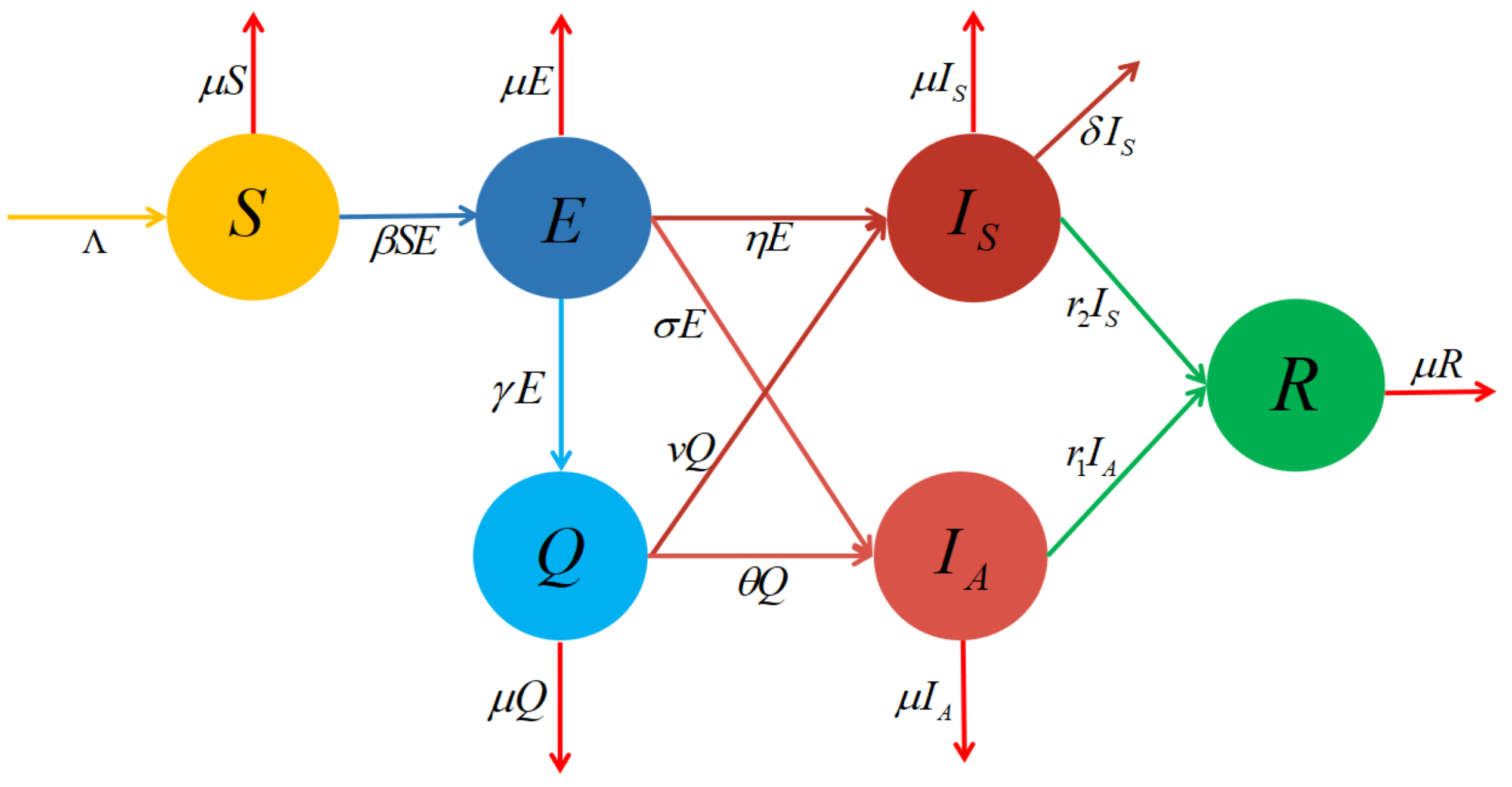
3. Model Description

According to the integer order infectious disease model in the literature [31], divide the crowd into six categories: $S\left(t\right),E\left(t\right),Q\left(t\right),I_A\left(t\right),I_S\left(t\right),R\left(t\right)$. They represent susceptible people, exposed people, isolated people, asymptomatic infected people, symptomatic infected people, and recovered people. Let N represent the total human population. Based on the above description we can obtain: $N\left(t\right)=S\left(t\right)+E\left(t\right)+Q\left(t\right)+I_A\left(t\right)+I_S\left(t\right)+R\left(t\right).$

When susceptible people are infected with infectious diseases, some infected people will be detected and isolated by security personnel. The isolated people are already infected people, but they will lose the ability to spread infectious diseases at the social level. All infected people are asymptomatic infected people or symptomatic infected people, and will be treated by different treatment schemes. The specific process is shown in Figure 1, in which $\mathsf{\Lambda }$ represents the net rate of population increase, $\mu$ the natural mortality rate, $\beta$ the prevalence of the infectious disease, $\gamma$ the detection isolation rate, $\sigma$ the asymptomatic rate of transmission, $\theta$ the symptomatic transmission rate, $\eta$ the isolated population’s transmission rate to people who become asymptomatic, v the isolated population’s transmission rate to people who become symptomatic, $\delta$ the unnatural death rate due to the infectious disease, $r_1$, the period of symptomatic infection, $r_2$ the period of asymptomatic infection.

Based on the disease integer-order model in the literature [31], this paper reconstructs the disease fractional order model, and considers the saturation of the pathogenicity rate (m is the saturation factor) and the infection incubation period $\tau$, and proposes the following system.

$$\left\{\begin{array}{c}{}^c{D}_t^{\alpha }S\left(t\right)=\mathsf{\Lambda }-\mu S\left(t\right)-\frac{\beta S\left(t\right)E(t-\tau )}{1+mS\left(t\right)},\hfill \\ {}^c{D}_t^{\alpha }E\left(t\right)=\frac{\beta S\left(t\right)E(t-\tau )}{1+mS\left(t\right)}-(\gamma +\mu +\eta +\sigma )E\left(t\right),\hfill \\ {}^c{D}_t^{\alpha }Q\left(t\right)=\gamma E\left(t\right)-(\mu +vs.+\theta )Q\left(t\right),\hfill \\ {}^c{D}_t^{\alpha }{I}_A\left(t\right)=\sigma E\left(t\right)+\theta Q\left(t\right)-(\mu +r_1)I_A\left(t\right),\hfill \\ {}^c{D}_t^{\alpha }{I}_S\left(t\right)=\eta E\left(t\right)+vQ\left(t\right)-(\delta +\mu +r_2)I_S\left(t\right),\hfill \\ {}^c{D}_t^{\alpha }R\left(t\right)=r_1{I}_A\left(t\right)+r_2{I}_S\left(t\right)-\mu R\left(t\right).\hfill \end{array}\right.$$

(7)

where $\alpha \in (0,1]$ and the initial conditions are as follows:

$$\begin{array}{c}S\left(t_0\right)=S_{t_0}\ge 0,E\left(t\right)=\varphi \left(t\right)\ge 0,Q\left(t_0\right)=Q_{t_0}\ge 0,\hfill \\ I_A\left(t_0\right)={I_A}_{t_0}\ge 0,I_S\left(t_0\right)={I_S}_{t_0}\ge 0,R\left(t_0\right)=R_{t_0}\ge 0,\hfill \end{array}$$

(8)

where $t\in \left(-\tau ,t_0\right].$

4. Basic Properties

4.1. Invariant Region and Boundedness

We explore the dynamic analysis of the model in a feasible area $\mathsf{\Omega }$, such that

$$\mathsf{\Omega }=\left\{(S\left(t\right),E\left(t\right),Q\left(t\right),I_A\left(t\right),I_S\left(t\right),R\left(t\right))\in {\mathbb{R}}_{+}^6:0\le N\left(t\right)\le \frac{\mathsf{\Lambda }}{\mu }\right\}.$$

(9)

Theorem 1.

If the initial conditions are non-negative, then Ω is the positive invariant set of the system (7).

If the theorem holds, then it can be seen from the theorem that the model proposed in this article performs well in epidemiology. We proceed to prove the correctness of the theorem below.

Proof. 

After adding the population components, the total population is as follows.

$${}^c{D}_t^{\alpha }N\left(t\right)={}^c{D}_t^{\alpha }S\left(t\right)+{}^c{D}_t^{\alpha }E\left(t\right)+{}^c{D}_t^{\alpha }Q\left(t\right)+{}^c{D}_t^{\alpha }{I}_A\left(t\right)+{}^c{D}_t^{\alpha }{I}_S\left(t\right)+{}^c{D}_t^{\alpha }R\left(t\right).$$

(10)

Bringing system (7) into the above equation and from (9), we can get

$${}^c{D}_t^{\alpha }N\left(t\right)+\mu N\left(t\right)\le \mathsf{\Lambda },$$

(11)

After a Laplace transformation, we can get

$$N\left(s\right)\le N\left(0\right)\frac{s^{\alpha -1}}{s^{\alpha }+\mu }+\frac{\mathsf{\Lambda }}{s(s^{\alpha }+\mu )},$$

(12)

Next, we consider using the inverse Laplace transform. We can calculate

$$N\left(t\right)\le (N\left(0\right)-\frac{\mathsf{\Lambda }}{\mu })E_{\alpha ,1}(-\mu t^{\alpha })+\frac{\mathsf{\Lambda }}{\mu }.$$

(13)

Therefore, when the initial conditions in $\mathsf{\Omega }$ are non-negative, the solution of the model is still in $\mathsf{\Omega }$, so the area $\mathsf{\Omega }$ is positive invariant and attracts all the solutions in ${\mathbb{R}}_{+}^6$. Furthermore, because for $\forall t>0$, satisfying the Mittag–Leffler function is bounded, and $\underset{t\to \infty }{lim}{E}_{\alpha ,1}(-\mu t^{\alpha })=0$, the conclusion is drawn from the above: $\mathsf{\Omega }$ is the positive invariant region of the system (7), and the solution of the system is bounded. □

4.2. Solution Nonnegativity

Theorem 2.

If the initial conditions are non-negative, the solution of system (7) is nonnegative for all $\forall t>t_0$.

Proof. 

In order to prove the non-negativity of the solution, we adopt the method of proof by contradiction. The specific proof process is divided into the following three parts.

Part 1. Prove that $S\left(t\right)>0$, for $\forall t>t_0$.

Suppose there is $t^{*}$, which can satisfy $S\left(t^{*}\right)=0$, and $S\left(t\right)<0$ for $\forall t\in (t^{*},t^{*}+\xi ]$, where $\xi$ is a positive number infinitely close to $t^{*}$.

From the assumptions, we can get ${}^c{D}_t^{\alpha }S\left(t^{*}\right)=\mathsf{\Lambda }>0$; then we can get ${}^c{D}_t^{\alpha }S\left(t\right)>0$ for $\forall t\in (t^{*},t^{*}+\xi ]$. Let ${}^c{D}_t^{\alpha }S\left(t\right)>cS\left(t\right)$, where $c>0$. Then we can get $S\left(t\right)>S\left(t^{*}\right)E_{\alpha ,1}\left(c{(t-t^{*})}^{\alpha }\right),$ for $\forall t\in (t^{*},t^{*}+\xi ]$ by calculation. Furthermore, because of $S\left(t^{*}\right)=0$, we get $S\left(t\right)>0$ for $\forall t\in (t^{*},t^{*}+\xi ]$, which contradicts the assumptions, so $S\left(t\right)>0$, for $\forall t>t_0$.

Part 2. Prove that $E\left(t\right)\ge 0$, for $\forall t>t_0$.

Similarly, suppose there is $t^{*}$, which can satisfy $E\left(t^{*}\right)=0$, and $E\left(t\right)<0$ for $\forall t\in (t^{*},t^{*}+\xi ]$. As the sign of ${}^c{D}_t^{\alpha }E\left(t\right)$ is uncertain, we will discuss it separately:

Case 1. If ${}^c{D}_t^{\alpha }E\left(t\right)\ge 0$ for $\forall t\in (t^{*},t^{*}+\xi ]$, then $E\left(t\right)>E\left(t^{*}\right)E_{\alpha ,1}\left(c{(t-t^{*})}^{\alpha }\right)$, which contradicts the assumptions.

Case 2. If ${}^c{D}_t^{\alpha }E\left(t\right)\le 0$ for $\forall t\in (t^{*},t^{*}+\xi ]$, at this time, we need to discuss the positive and negative situation of $E(t-\tau )$.

1. If $E(t-\tau )\ge 0$, then

$${}^c{D}_t^{\alpha }E\left(t\right)=\frac{\beta SE(t-\tau )}{1+mS}-(\gamma +\mu +\eta +\sigma )E\ge -(\gamma +\mu +\eta +\sigma )E\ge 0,$$

(14)

there is a contradiction here.

2. If $E(t-\tau )\le 0$, we can get $E(t-\tau )\ge E\left(t\right)$; then

$$\begin{array}{c}{}^c{D}_t^{\alpha }E\left(t\right)=\frac{\beta SE(t-\tau )}{1+mS}-(\gamma +\mu +\eta +\sigma )E\left(t\right)\hfill \\ \ge \frac{\beta SE}{1+mS}-(\gamma +\mu +\eta +\sigma )E\hfill \\ \ge \frac{\beta SE}{1+mS}\ge \frac{\beta }{m}E;\hfill \end{array}$$

(15)

after calculations, we can get $E\left(t\right)\ge E\left(t^{*}\right)E_{\alpha ,1}\left(\frac{\beta }{m}{(t-t^{*})}^{\alpha }\right),$ for $\forall t\in (t^{*},t^{*}+\xi ]$. At this time there is a contradiction. Thus, $E\left(t\right)\ge 0$, for $\forall t>t_0$.

Part 3. Combining part 1 and the part 2 of the proof process, we can get $Q\left(t\right)\ge 0,I_A\left(t\right)\ge 0,I_S\left(t\right)\ge 0,R\left(t\right)\ge 0,$ for $\forall t>t_0$.

In summary, the solution of the system is proved to be non-negative. □

4.3. Disease-Free Equilibrium (DFE)

The equilibrium point $(S_{*},E_{*},Q_{*},{I_A}_{*},{I_S}_{*},R_{*})$ of system (7) can be obtained by solving the following equations.

$$\left\{\begin{array}{c}\mathsf{\Lambda }-\mu S_{*}-\frac{\beta S_{*}{E}_{*}}{1+m{S}_{*}}=0,\hfill \\ \frac{\beta S_{*}{E}_{*}}{1+m{S}_{*}}-(\gamma +\mu +\eta +\sigma )E_{*}=0,\hfill \\ \gamma E_{*}-(\mu +vs.+\theta )Q_{*}=0,\hfill \\ \sigma E_{*}+\theta Q_{*}-(\mu +r_1){I_A}_{*}=0,\hfill \\ \eta E_{*}+v{Q}_{*}-(\delta +\mu +r_2){I_S}_{*}=0,\hfill \\ r_1{I_A}_{*}+r_2{I_S}_{*}-\mu R_{*}=0.\hfill \end{array}\right.$$

(16)

In Equation (16), let $E_{*}=0,Q_{*}=0,{I_A}_{*}=0,{I_S}_{*}=0,R_{*}=0$ to get the disease-free equilibrium point (DFE), denoted by $E_0$; that is,

$$E_0=(\frac{\mathsf{\Lambda }}{\mu },0,0,0,0,0).$$

(17)

We use ${\mathcal{R}}_0$ to represent the expected value of the infection rate per time unit, that is, the basic reproduction number. Next, we use the next-generation matrix method to find ${\mathcal{R}}_0$.

$${}^c{D}_t^{\alpha }X=F\left(x\right)-V\left(x\right),$$

(18)

where

$$F\left(x\right)=\left(\begin{array}{c}\frac{\beta SE}{1+mS}\hfill \\ 0\hfill \\ 0\hfill \\ 0\hfill \end{array}\right),V\left(x\right)=\left(\begin{array}{c}(\gamma +\mu +\eta +\sigma )E\hfill \\ -\gamma E+(\mu +vs.+\theta )Q\hfill \\ -\sigma E-\theta Q+(\mu +r_1)I_A\hfill \\ -\eta E-vQ+(\delta +\mu +r_2)I_S\hfill \end{array}\right).$$

The Jacobian matrix at $E_0$ is denoted by F, V, which is

$$F=\left(\begin{array}{cccc}\frac{\beta \mathsf{\Lambda }}{\mu +m\mathsf{\Lambda }}& 0& 0& 0\\ 0& 0& 0& 0\\ 0& 0& 0& 0\\ 0& 0& 0& 0\end{array}\right),V=\left(\begin{array}{cccc}\gamma +\mu +\eta +\sigma & 0& 0& 0\\ -\gamma & \mu +vs.+\theta & 0& 0\\ -\sigma & -\theta & \mu +r_1& 0\\ -\eta & -v& 0& \delta +\mu +r_2\end{array}\right).$$

Then we can get the basic reproduction number

$${\mathcal{R}}_0=\rho \left(F{V}^{-1}\right)=\frac{\beta \mathsf{\Lambda }}{A(\mu +m\mathsf{\Lambda })}.$$

(19)

where $A=\gamma +\mu +\eta +\sigma .$

4.4. Existence of Endemic Equilibrium Point

In this section, we focus on studying the existence of local equilibrium points. Let the local balance point be $E^{*}=(S_{*},E_{*},Q_{*},{I_A}_{*},{I_S}_{*},R_{*})$. Then we can acquire the following theorem.

Theorem 3.

When ${\mathcal{R}}_0>1$ and $\beta -mA>0$, the system (7) has its own unique balance point:

$$E^{*}=(\frac{A}{\beta -mA},a({\mathcal{R}}_0-1),b({\mathcal{R}}_0-1),c({\mathcal{R}}_0-1),d({\mathcal{R}}_0-1),\frac{c{r}_1+d{r}_2}{\mu }({\mathcal{R}}_0-1)),$$

where

$$\begin{array}{c}a=\frac{\mu +m\mathsf{\Lambda }}{\beta -mA},b=\frac{\gamma (\mu +m\mathsf{\Lambda })}{(\mu +vs.+\theta )(\beta -mA)},\hfill \\ c=\frac{(\theta \gamma +\sigma (\mu +vs.+\theta \left)\right)(\mu +m\mathsf{\Lambda })}{(\mu +r_1)(\mu +vs.+\theta )(\beta -mA)},d=\frac{(v\gamma +\eta (\mu +vs.+\theta \left)\right)(\mu +m\mathsf{\Lambda })}{(\delta +\mu +r_2)(\mu +vs.+\theta )(\beta -mA)}.\hfill \end{array}$$

Proof. 

First, solve the second equation in (16) to obtain

$$S_{*}=\frac{A}{\beta -mA}.$$

(20)

By substituting Equation (20) into the first equation in (16), we can get

$$E_{*}=\frac{\mu +m\mathsf{\Lambda }}{\beta -mA}({\mathcal{R}}_0-1)=a({\mathcal{R}}_0-1).$$

(21)

By combining and substituting Equations (20) and (21) into the third equation in (16), it is easy to get

$$Q_{*}=\frac{\gamma (\mu +m\mathsf{\Lambda })}{(\mu +vs.+\theta )(\beta -mA)}({\mathcal{R}}_0-1)=b({\mathcal{R}}_0-1).$$

(22)

Then, by substituting Formulas (21) and (22) into the fourth and fifth equations in (16), we can calculate

$${I_A}_{*}=\frac{(\theta \gamma +\sigma (\mu +vs.+\theta \left)\right)(\mu +m\mathsf{\Lambda })}{(\mu +r_1)(\mu +vs.+\theta )(\beta -mA)}({\mathcal{R}}_0-1)=c({\mathcal{R}}_0-1).$$

(23)

$${I_S}_{*}=\frac{(v\gamma +\eta (\mu +vs.+\theta \left)\right)(\mu +m\mathsf{\Lambda })}{(\delta +\mu +r_2)(\mu +vs.+\theta )(\beta -mA)}({\mathcal{R}}_0-1)=d({\mathcal{R}}_0-1).$$

(24)

Finally, the relationship between the last equation in (16) and the first two equations can be obtained.

$$R_{*}=\frac{c{r}_1+d{r}_2}{\mu }({\mathcal{R}}_0-1).$$

(25)

In summary, when ${\mathcal{R}}_0>1$ and $\beta -mA>0$, every element of $E^{*}$ is positive and unique, so it is a unique balance point of system (7). □

5. Stability Analysis

Before studying the stability, we first derive the linearized system of the system (7) at the equilibrium point as follows:

$$\left\{\begin{array}{c}{}^c{D}_t^{\alpha }S\left(t\right)=-(\mu +\frac{\beta E_{*}}{{(1+m{S}_{*})}^2})S\left(t\right)-\frac{\beta S_{*}}{1+m{S}_{*}}E(t-\tau ),\hfill \\ {}^c{D}_t^{\alpha }E\left(t\right)=\frac{\beta E_{*}}{{(1+m{S}_{*})}^2}S\left(t\right)+\frac{\beta S_{*}}{1+m{S}_{*}}E(t-\tau )-(\gamma +\mu +\eta +\sigma )E\left(t\right),\hfill \\ {}^c{D}_t^{\alpha }Q\left(t\right)=\gamma E\left(t\right)-(\mu +vs.+\theta )Q\left(t\right),\hfill \\ {}^c{D}_t^{\alpha }{I}_A\left(t\right)=\sigma E\left(t\right)+\theta Q\left(t\right)-(\mu +r_1)I_A\left(t\right),\hfill \\ {}^c{D}_t^{\alpha }{I}_S\left(t\right)=\eta E\left(t\right)+vQ\left(t\right)-(\delta +\mu +r_2)I_S\left(t\right),\hfill \\ {}^c{D}_t^{\alpha }R\left(t\right)=r_1{I}_A\left(t\right)+r_2{I}_S\left(t\right)-\mu R\left(t\right).\hfill \end{array}\right.$$

(26)

Take the Laplace transform on both sides of (26) to get

$$\left\{\begin{array}{c}{s}^{\alpha }L\left[S\left(s\right)\right]-s^{\alpha -1}S\left(0\right)=-(\mu +\frac{\beta E_{*}}{{(1+m{S}_{*})}^2})L\left[S\left(s\right)\right]-\frac{\beta S_{*}}{1+m{S}_{*}}{e}^{-s\tau }(L\left[E\left(s\right)\right]+{\int }_{-\tau }^0{e}^{-st}\varphi \left(t\right)dt),\hfill \\ s^{\alpha }L\left[E\left(s\right)\right]-s^{\alpha -1}E\left(0\right)=\frac{\beta E_{*}}{{(1+m{S}_{*})}^2}L\left[S\left(s\right)\right]+\frac{\beta S_{*}}{1+m{S}_{*}}{e}^{-s\tau }(L\left[E\left(s\right)\right]+{\int }_{-\tau }^0{e}^{-st}\varphi \left(t\right)dt)\hfill \\ -(\gamma +\mu +\eta +\sigma )L\left[E\right(s\left)\right],\hfill \\ s^{\alpha }L\left[Q\left(s\right)\right]-s^{\alpha -1}Q\left(0\right)=\gamma L\left[E\left(s\right)\right]-(\mu +vs.+\theta )L\left[Q\left(s\right)\right],\hfill \\ s^{\alpha }L\left[I_A\left(s\right)\right]-s^{\alpha -1}{I}_A\left(0\right)=\sigma L\left[E\left(s\right)\right]+\theta L\left[Q\left(s\right)\right]-(\mu +r_1)L\left[I_A\left(s\right)\right]\hfill \\ s^{\alpha }L\left[I_S\left(s\right)\right]-s^{\alpha -1}{I}_S\left(0\right)=\eta L\left[E\left(s\right)\right]+vL\left[Q\left(s\right)\right]-(\delta +\mu +r_2)L\left[I_S\left(s\right)\right],\hfill \\ s^{\alpha }L\left[R\left(s\right)\right]-s^{\alpha -1}R\left(0\right)=r_{1}L\left[I_A\left(s\right)\right]+r_{2}L\left[I_S\left(s\right)\right]-\mu L\left[R\left(s\right)\right].\hfill \end{array}\right.$$

(27)

The following form can replace the system (27):

$$\begin{array}{c}\mathsf{\Delta }\left(s\right)·{(L\left[S\left(s\right)\right],L\left[E\left(s\right)\right],L\left[Q\left(s\right)\right],L\left[I_A\left(s\right)\right],L\left[I_S\left(s\right)\right],L\left[R\left(s\right)\right])}^{\mathrm{T}}\hfill \\ ={(b_1\left(s\right),b_2\left(s\right),b_3\left(s\right),b_4\left(s\right),b_5\left(s\right),b_6\left(s\right))}^{\mathrm{T}}\hfill \end{array}$$

where

$$\begin{array}{c}\mathsf{\Delta }\left(s\right)=\left(\begin{array}{cccc}{s}^{\alpha }+\mu +\frac{\beta E_{*}}{{(1+m{S}_{*})}^2}& \frac{\beta S_{*}}{1+m{S}_{*}}{e}^{-s\tau }& \cdots & 0\\ -\frac{\beta E_{*}}{{(1+m{S}_{*})}^2}& s^{\alpha }-\frac{\beta S_{*}}{1+m{S}_{*}}{e}^{-s\tau }+A& \cdots & 0\\ ⋮& ⋮& \ddots & ⋮\\ 0& 0& \cdots & s^{\alpha }+\mu \end{array}\right)\hfill \end{array}$$

$$\begin{array}{c}{b}_1\left(s\right)=s^{\alpha -1}S\left(0\right)-\frac{\beta S_{*}}{1+m{S}_{*}}{e}^{-s\tau }{\int }_{-\tau }^0{e}^{-st}\varphi \left(t\right)dt,\hfill \\ b_2\left(s\right)=s^{\alpha -1}E\left(0\right)+\frac{\beta S_{*}}{1+m{S}_{*}}{e}^{-s\tau }{\int }_{-\tau }^0{e}^{-st}\varphi \left(t\right)dt,\hfill \\ b_3\left(s\right)=s^{\alpha -1}Q\left(0\right),b_4\left(s\right)=s^{\alpha -1}{I}_A\left(0\right),\hfill \\ b_5\left(s\right)=s^{\alpha -1}{I}_S\left(0\right),b_6\left(s\right)=s^{\alpha -1}R\left(0\right).\hfill \end{array}$$

As $\mathsf{\Delta }\left(s\right)$ is the characteristic matrix of the system (27), the eigenvalue distribution of $det\left(\mathsf{\Delta }\right(s\left)\right)$ can be used to study the stable nature of the system.

5.1. Local Stability of DFE

Theorem 4.

When ${\mathcal{R}}_0<1$, the DFE of the system (7) is locally asymptotically stable for any τ.

Proof. 

Put $E_0$ into $\mathsf{\Delta }\left(s\right)$. One can get the characteristic equation $det\left({\mathsf{\Delta }}_0\left(s\right)\right)$ of the system at $E_0$, and make $det\left({\mathsf{\Delta }}_0\left(s\right)\right)=0$ easy to calculate. Substituting $\lambda =s^{\alpha }$ into the equation provides the following equation:

$$(\lambda -\frac{\beta \mathsf{\Lambda }}{\mu +m\mathsf{\Lambda }}{e}^{-s\tau }+A)(\lambda +\mu +vs.+\theta )(\lambda +\mu +r_1)(\lambda +\delta +\mu +r_2){(\lambda +\mu )}^2=0.$$

(28)

In Equation (28), except for the first factor, it is obvious that

$${\lambda }_2=-(\mu +vs.+\theta )<0,{\lambda }_3=-(\mu +r)<0,{\lambda }_4=-(\delta +\mu +r_2)<0,{\lambda }_5={\lambda }_6=-\mu <0.$$

1. When $\tau =0$, ${\lambda }_1=\frac{\beta \mathsf{\Lambda }}{\mu +m\mathsf{\Lambda }}-A=A({\mathcal{R}}_0-1)$ for ${\mathcal{R}}_0<1.$

2. When $\tau \ne 0$, let $\lambda ={\left(i\omega \right)}^{\alpha }$, put in the first factor of the Equation (28) to get

$${\omega }^{\alpha }(cos\frac{\alpha \pi }{2}+isin\frac{\alpha \pi }{2})-\frac{\beta \mathsf{\Lambda }}{\mu +m\mathsf{\Lambda }}(cos\omega \tau -isin\omega \tau )+A=0$$

(29)

Separating the real and imaginary parts of Equation (29) provides

$$\left\{\begin{array}{c}{\omega }^{\alpha }cos\frac{\alpha \pi }{2}+A=\frac{\beta \mathsf{\Lambda }}{\mu +m\mathsf{\Lambda }}cos\omega \tau ,\hfill \\ -{\omega }^{\alpha }sin\frac{\alpha \pi }{2}=\frac{\beta \mathsf{\Lambda }}{\mu +m\mathsf{\Lambda }}sin\omega \tau .\hfill \end{array}\right.$$

(30)

After summing the squares of the two sides, it can be simplified to get

$${\omega }^{2\alpha }+2A{\omega }^{\alpha }cos\frac{\alpha \pi }{2}+A(A+\frac{\beta \mathsf{\Lambda }}{\mu +m\mathsf{\Lambda }})(1-{\mathcal{R}}_0)=0.$$

(31)

It can be seen that when ${\mathcal{R}}_0<1$, Equation (31) has no positive roots—that is, $\left|arg\left({\omega }_{1,2}^{\alpha }\right)\right|>\frac{\alpha \pi }{2}$. By combining the above discussion, we can get $\left|arg\left({\lambda }_i\right)\right|>\frac{\alpha \pi }{2}$ for $i=1,2,3,4,5,6$. According to the Lemma 1, we can complete the proof of the Theorem 4. □

Remark 1.

We consider the method of constructing an appropriate Lyapunov function: $V\left(t\right)=Y_{1}E\left(t\right)+Y_{2}Q\left(t\right)$. The coefficients($Y_1,Y_2$) are to be determined. The Caputo-fractional derivative of $V\left(t\right)$, along system (7) when $\tau =0$, is

$$\begin{array}{c}{}^c{D}_t^{\alpha }V\left(t\right)=Y_1{}^c{D}_t^{\alpha }E\left(t\right)+Y_2{}^c{D}_t^{\alpha }Q\left(t\right)\hfill \\ =Y_1\frac{\beta SE}{1+mS}-Y_{1}AE+Y_2\gamma E-Y_2(\mu +vs.+\theta )Q\hfill \\ \le (Y_1\frac{\beta \mathsf{\Lambda }}{\mu +m\mathsf{\Lambda }}-Y_{1}A+Y_2\gamma )E-Y_2(\mu +vs.+\theta )Q\hfill \\ =Y_{1}A(\frac{\beta \mathsf{\Lambda }{Y}_1+Y_2\gamma (\mu +m\mathsf{\Lambda })}{Y_{1}A(\mu +m\mathsf{\Lambda })}-1)E-Y_2(\mu +vs.+\theta )Q.\hfill \end{array}$$

(32)

Let $Y_1=\frac{\mu }{\mu +m\mathsf{\Lambda }},Y_2=\frac{m\beta {\mathsf{\Lambda }}^2}{\gamma {(\mu +m\mathsf{\Lambda })}^2}.$ By substituting them into the above formula, we can get

$${}^c{D}_t^{\alpha }V\left(t\right)\le \frac{A\mu E}{\mu +m\mathsf{\Lambda }}({\mathcal{R}}_0-1)-\frac{m\beta {\mathsf{\Lambda }}^2(\mu +vs.+\theta )}{\gamma {(\mu +m\mathsf{\Lambda })}^2}Q.$$

(33)

Obviously get ${}^c{D}_t^{\alpha }V\left(t\right)\le 0$ for ${\mathcal{R}}_0<1$. The equals sign is true if and only if $E\left(t\right)=0,Q\left(t\right)=0$. Thus, $(E,Q)\to (0,0)$ as $t\to \infty$. By substituting $E\left(t\right)=0,Q\left(t\right)=0$ into the system, we can get $S\to \frac{\mathsf{\Lambda }}{\mu }$ and $Q,I_A,I_S\to 0$ as $t\to \infty$. Therefore, from the Lyapunov stability theorem of fractional order, we can know that when $t\to \infty$, the system tends to the point $E_0$ in the feasible region, so DFE of the system (7) is global progressive stability when $\tau =0$.

5.2. Local Stability Analysis of the Endemic Equilibrium

In this section, we study the local asymptotic stability of the local equilibrium point of system (7). Put $E^{*}$ into $\mathsf{\Delta }\left(s\right)$. Then, we can get the characteristic equation $det\left({\mathsf{\Delta }}^{*}\left(s\right)\right)$ of the system at $E^{*}$, and make $det\left({\mathsf{\Delta }}^{*}\left(s\right)\right)=0$ easy to calculate. By substituting $a_1=\frac{\beta E_{*}}{{(1+m{S}_{*})}^2}$ and $\lambda =s^{\alpha }$ into the equation, can get the following equation.

$$\begin{array}{c}det\left({\mathsf{\Delta }}^{*}\left(s\right)\right)=[(\lambda +\mu +a_1)(\lambda -A{e}^{-s\tau }+A)+A{e}^{-s\tau }{a}_1](\lambda +\mu +vs.+\theta )\hfill \\ (\lambda +\mu +r_1)(\lambda +\delta +\mu +r_2)(\lambda +\mu )=0\hfill \end{array}$$

(34)

From the previous proof, we can get the characteristic roots of Equation (34) except for the first factor, and ${\lambda }_i<0$ for $i=3,4,5,6$.

1. When $\tau =0$, the first factor in Equation (34) is changed to

$${\lambda }^2+\lambda (\mu +a_1)+A{a}_1=0.$$

(35)

As $\mu +a_1>0,A{a}_1>0$, it can be seen that the one-dimensional quadratic equation above has no positive roots.

2. When $\tau \ne 0$, let $\lambda ={\left(i\omega \right)}^{\alpha }$. Put in the first factor of Equation (34) and separate the real part and the imaginary part to obtain the following equation:

$$\left\{\begin{array}{c}{\omega }^{2\alpha }cos\alpha \pi +d_2{\omega }^{\alpha }cos\frac{\alpha \pi }{2}+d_4=d_1{\omega }^{\alpha }cos(\frac{\alpha \pi }{2}-\omega \tau )+d_{3}cos\omega \tau ,\hfill \\ {\omega }^{2\alpha }sin\alpha \pi +d_2{\omega }^{\alpha }sin\frac{\alpha \pi }{2}=-d_1{\omega }^{\alpha }sin(\frac{\alpha \pi }{2}-\omega \tau )-d_{3}sin\omega \tau .\hfill \end{array}\right.$$

(36)

where $d_1=A,d_2=A+\mu +a_1,d_3=-\mu A,d_4=(\mu +a_1)A$.

After summing the squares of the two sides, it can be simplified to

$${\omega }^{4\alpha }+(2d_{2}cos\frac{\alpha \pi }{2}){\omega }^{3\alpha }+(d_2^2+2d_{4}cos\alpha \pi -d_1^2){\omega }^{2\alpha }+2(d_2{d}_4-d_1{d}_3){\omega }^{\alpha }+(d_4^2-d_3^2)=0.$$

(37)

According to the judgment method of the unary quartic equation, it can be concluded that when $d_2^2+2d_{4}cos\alpha \pi -d_1^2>0,d_2{d}_4-d_1{d}_3>0,d_4^2-d_3^2>0,$ the equation has no positive roots. Furthermore, after $d_i(i=1,2,3,4)$ is brought in, the above conditions can be met. Therefore, all the characteristic roots of the characteristic equation $det\left({\mathsf{\Delta }}^{*}\left(s\right)\right)=0$ satisfy $\left|arg\left({\lambda }_i\right)\right|>\frac{\alpha \pi }{2},i=1,2,3,4,5,6$, and we can get the following theorem.

Theorem 5.

When the endemic equilibrium point $E^{*}$ exists, that is, ${\mathcal{R}}_0>1$ and $\beta -m\mathsf{\Lambda }>0$, the endemic equilibrium point of the system (7) is locally asymptotically stable for any τ.

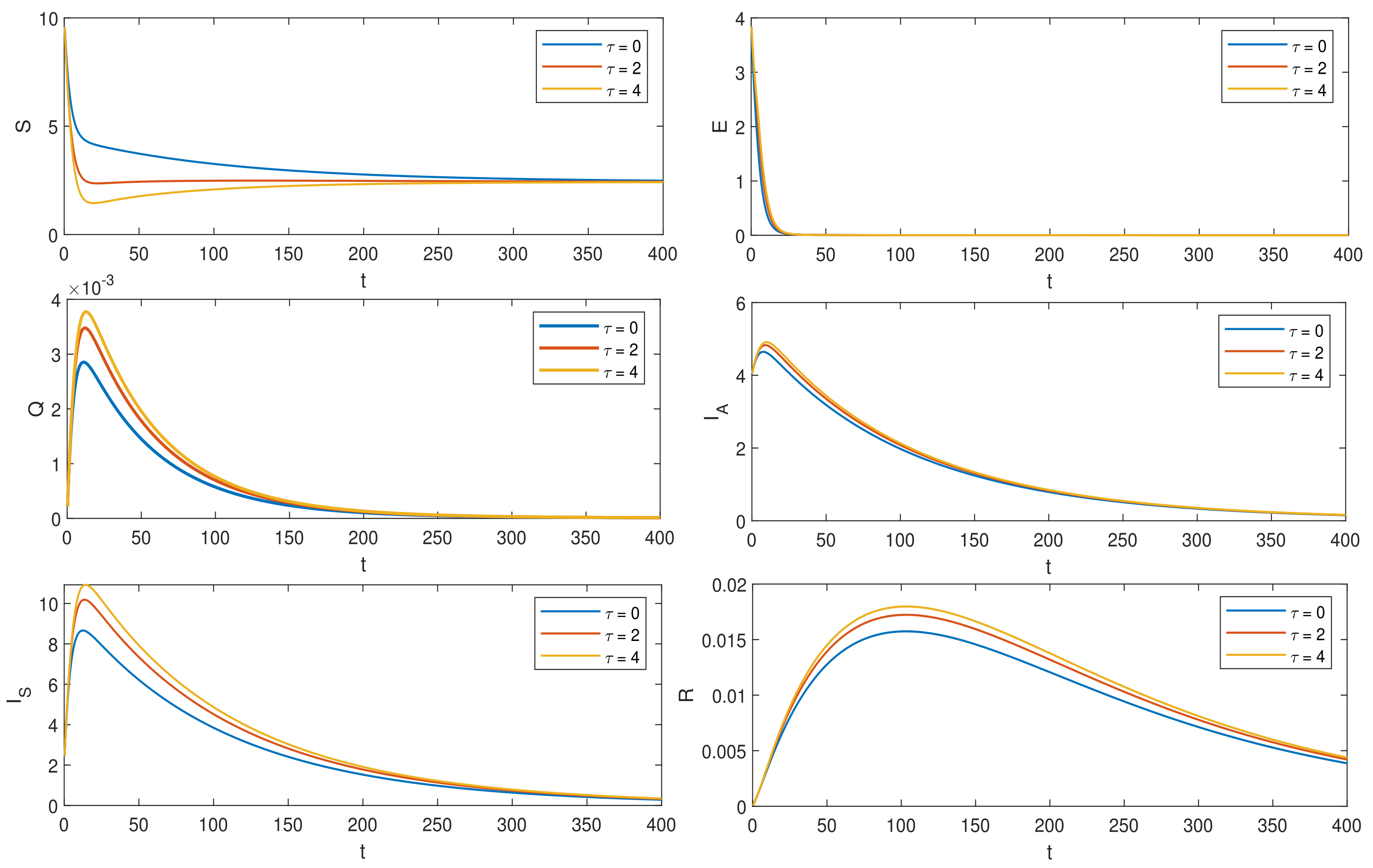
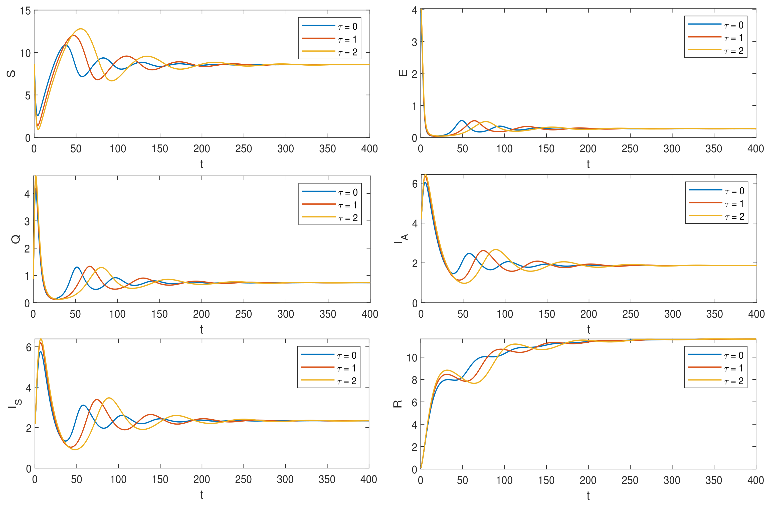
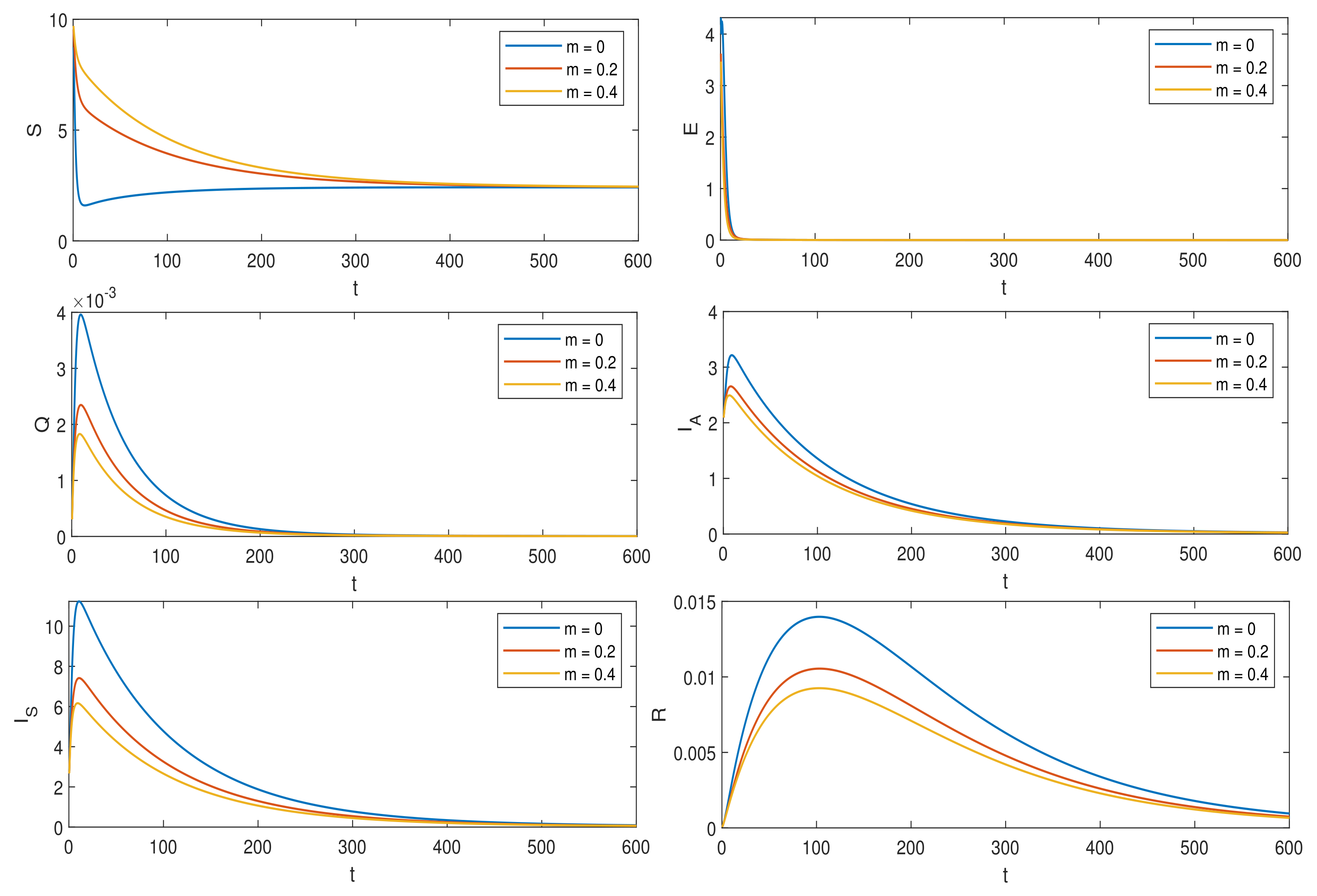
6. Numerical Simulations

In order to illustrate the correctness of the conclusions of the text, the initial conditions for the state variables were: $S\left(0\right)=10,E\left(0\right)=4,Q\left(0\right)=0,I_A\left(0\right)=4,I_S\left(0\right)=2,R\left(0\right)=0,$ and we used two sets of data to conduct numerical simulations, as shown in the following table.

The first set of baseline values in

Table 1. System parameter values used in the simulation.

Parameters	$\mathbf{\Lambda }$	$\mathit{\mu }$	$\mathit{\beta }$	m	$\mathit{\sigma }$	$\mathit{\gamma }$
1	0.02537	0.0106	0.0805	0.12	0.0668	2.0138 $\times {10}^{-4}$
2	0.5	0.018	0.3	0.12	0.25	0.8
Parameters	$\mathbf{\eta }$	$\mathbf{\theta }$	$\mathit{v}$	$\mathbf{\delta }$	${\mathit{r}}_{\mathbf{1}}$	${\mathit{r}}_{\mathbf{2}}$
1	0.4478	0.0101	3.2084$\times {10}^{-4}$	1.6728$\times {10}^{-5}$	5.7341$\times {10}^{-5}$	1.6728$\times {10}^{-5}$
2	0.2	0.08	0.2	0.018	0.05	0.05

was provided by the literature [31]. It can be obtained that ${\mathcal{R}}_0=0.2849<1$ at this time. The simulation results are shown in Figure 2. We set the order of the system to $\alpha =0.98$, and selected $\tau =0,\tau =2,\tau =4$. It can be seen from Figure 2 that the disease-free equilibrium point $E_0$ is locally asymptotically stable.

In order to satisfy the situation of ${\mathcal{R}}_0>1$, we selected the second set of data in Table 1 to obtain ${\mathcal{R}}_0=1.5166$ at this time and the endemic equilibrium point $E^{*}=(8.8768,0.2726,0.7317,1.8629,2.3356,11.6626)$. The results of the simulation are shown in Figure 3. It can be seen in Figure 3 that the endemic equilibrium point $E^{*}$ is locally asymptotically stable. We set the order of the system to 0.98, and selected $\tau =0,\tau =1,\tau =2$.

The biological significance of the parameter m is the epidemic control measures imposed on the susceptible population S. $\gamma$ is the isolation rate (the efficiency of detecting infected individuals); i.e., the greater the control input, the greater the values of m and $\gamma$, and the better the epidemic control—the faster convergence to zero for asymptomatic and symptomatic infected individuals. See Figure 4 and Figure 5.

When $m=0$ and no time lag is considered ($\tau =0$), the model is essentially the same as the integer order model in the literature [31] except for the fractional order derivatives; and as obtained through Figure 4, increasing the value of m results in faster convergence, indicating that the epidemic ends earlier with increased control of the susceptible population. In addition, when m increases, the formula for ${\mathcal{R}}_0$ shows that the value of R0 is inversely proportional to m. The larger m is, the smaller ${\mathcal{R}}_0$ is, which theoretically illustrates the role of the control measure m, which can adjust the size of m making ${\mathcal{R}}_0>1$ change to ${\mathcal{R}}_0<1$.

7. Conclusions

In this paper, a fractional infectious disease model with saturated incidence and time delay was proposed. After obtaining the invariant region of the model and the non-negativity of the model solution, we found that that if the initial conditions are non-negative, then $\mathsf{\Omega }$ is the positive invariant set of the system. The basic replication number ${\mathcal{R}}_0$ is obtained by the next-generation matrix method. The disease-free equilibrium point $E_0$ can be calculated, and the endemic equilibrium point $E^{*}$ exists and is unique When ${\mathcal{R}}_0>1$ and $\beta -mA>0$. We also found that when ${\mathcal{R}}_0<1$, the DFE of the system is locally asymptotically stable for any $\tau$, and when the endemic equilibrium point $E^{*}$ exists, then it is locally asymptotically stable for any $\tau$. Based on the influences of the coefficients m and $\gamma$ on the system, it can be seen that human technological interventions can play a significant role in controlling the spread of infectious diseases—for example, vaccination, isolation measures, etc.

References

1. Unkel, S.; Farrington, C.P.; Garthwaite, P.H.; Robertson, C.; Andrews, N. Statistical methods for the prospective detection of infectious disease outbreaks: A review. J. R. Stat. Soc. Ser. A (Stat. Soc.) 2012, 175, 49–82. [Google Scholar] [CrossRef] [Green Version]
2. Nasution, H.; Jusuf, H.; Ramadhani, E.; Husein, I. Model of Spread of Infectious Disease. Syst. Rev. Pharm. 2020, 11, 685–689. [Google Scholar]
3. Bjørnstad, O.N.; Finkenstädt, B.F.; Grenfell, B.T. Dynamics of measles epidemics: Estimating scaling of transmission rates using a time series SIR model. Ecol. Monogr. 2002, 72, 169–184. [Google Scholar] [CrossRef] [Green Version]
4. Yu, J.; Jiang, D.; Shi, N. Global stability of two-group SIR model with random perturbation. J. Math. Anal. Appl. 2009, 360, 235–244. [Google Scholar] [CrossRef] [Green Version]
5. Bentout, S.; Chen, Y.; Djilali, S. Global dynamics of an SEIR model with two age structures and a nonlinear incidence. Acta Appl. Math. 2021, 171, 1–27. [Google Scholar] [CrossRef]
6. Funk, S.; Camacho, A.; Kucharski, A.J.; Eggo, R.M.; Edmunds, W.J. Real-time forecasting of infectious disease dynamics with a stochastic semi-mechanistic model. Epidemics 2018, 22, 56–61. [Google Scholar] [CrossRef] [PubMed]
7. Dietz, K.; Heesterbeek, J.A.P. Daniel Bernoulli’s epidemiological model revisited. Math. Biosci. 2002, 180, 1–21. [Google Scholar] [CrossRef] [Green Version]
8. Ehrhardt, M.; Gašper, J.; Kilianová, S. SIR-based mathematical modeling of infectious diseases with vaccination and waning immunity. J. Comput. Sci. 2019, 37, 101027. [Google Scholar] [CrossRef]
9. Li, M.Y.; Graef, J.R.; Wang, L.; Karsai, J. Global dynamics of a SEIR model with varying total population size. Math. Biosci. 1999, 160, 191–213. [Google Scholar] [CrossRef] [Green Version]
10. Korobeinikov, A. Global properties of SIR and SEIR epidemic models with multiple parallel infectious stages. Bull. Math. Biol. 2009, 71, 75–83. [Google Scholar] [CrossRef]
11. López, L.; Rodo, X. A modified SEIR model to predict the COVID-19 outbreak in Spain and Italy: Simulating control scenarios and multi-scale epidemics. Results Phys. 2021, 21, 103746. [Google Scholar] [CrossRef]
12. Rossikhin, Y.A.; Shitikova, M.V. Applications of fractional calculus to dynamic problems of linear and nonlinear hereditary mechanics of solids. Appl. Mech. Rev. 1997, 50, 15–67. [Google Scholar] [CrossRef]
13. Povstenko, Y.Z. Thermoelasticity that uses fractional heat conduction equation. J. Math. Sci. 2009, 162, 296–305. [Google Scholar] [CrossRef]
14. Baillie, R.T.; Bollerslev, T.; Mikkelsen, H.O. Fractionally integrated generalized autoregressive conditional heteroskedasticity. J. Econom. 1996, 74, 3–30. [Google Scholar] [CrossRef]
15. Jafari, H.; Ganji, R.M.; Nkomo, N.S.; Lv, Y.P. A numerical study of fractional order population dynamics model. Results Phys. 2021, 27, 104456. [Google Scholar] [CrossRef]
16. Freeborn, T.J.; Critcher, S. Cole-impedance model representations of right-side segmental arm, leg, and full-body bioimpedances of healthy adults: Comparison of fractional-order. Fractal Fract. 2021, 5, 13. [Google Scholar] [CrossRef]
17. Amin, R.; Mahariq, I.; Shah, K.; Awais, M.; Elsayed, F. Numerical solution of the second order linear and nonlinear integro-differential equations using Haar wavelet method. Arab. J. Basic Appl. Sci. 2021, 28, 12–20. [Google Scholar] [CrossRef]
18. Naik, P.A.; Zu, J.; Owolabi, K.M. Modeling the mechanics of viral kinetics under immune control during primary infection of HIV-1 with treatment in fractional order. Phys. A Stat. Mech. Its Appl. 2020, 545, 123816. [Google Scholar] [CrossRef]
19. Liu, F.; Huang, S.; Zheng, S.; Wang, H.O. Stability Analysis and Bifurcation Control for a Fractional Order SIR Epidemic Model with Delay. In Proceedings of the 2020 39th Chinese Control Conference (CCC), Shenyang, China, 27–29 July 2020; pp. 724–729. [Google Scholar]
20. Jajarmi, A.; Yusuf, A.; Baleanu, D.; Inc, M. A new fractional HRSV model and its optimal control: A non-singular operator approach. Phys. A Stat. Mech. Its Appl. 2020, 547, 123860. [Google Scholar] [CrossRef]
21. Hoan, L.V.C.; Akinlar, M.A.; Inc, M.; Gómez-Aguilar, J.F.; Chu, Y.M.; Almohsen, B. A new fractional-order compartmental disease model. Alex. Eng. J. 2020, 59, 3187–3196. [Google Scholar] [CrossRef]
22. Ma, W.; Song, M.; Takeuchi, Y. Global stability of an SIR epidemicmodel with time delay. Appl. Math. Lett. 2004, 17, 1141–1145. [Google Scholar] [CrossRef] [Green Version]
23. Rihan, F.A.; Alsakaji, H.J.; Rajivganthi, C. Stochastic SIRC epidemic model with time-delay for COVID-19. Adv. Differ. Equ. 2020, 2020, 1–20. [Google Scholar] [CrossRef]
24. Kaddar, A. Stability analysis in a delayed SIR epidemic model with a saturated incidence rate. Nonlinear Anal. Model. Control. 2010, 15, 299–306. [Google Scholar] [CrossRef]
25. Liu, X.; Yang, L. Stability analysis of an SEIQV epidemic model with saturated incidence rate. Nonlinear Anal. Real World Appl. 2012, 13, 2671–2679. [Google Scholar] [CrossRef]
26. Ashcroft, P.; Lehtinen, S.; Angst, D.C.; Low, N.; Bonhoeffer, S. Quantifying the impact of quarantine duration on COVID-19 transmission. eLife 2021, 10, e63704. [Google Scholar] [CrossRef]
27. Marchi, S.; Simonetta, V.; Remarque, E.; Ruello, A.; Bombardieri, E.; Bollati, V.; Trombetta, C. Characterization of antibody response in asymptomatic and symptomatic SARS-CoV-2 infection. PLoS ONE 2021, 16, e0253977. [Google Scholar] [CrossRef]
28. Wang, X.; Wang, Z.; Xia, J. Stability and bifurcation control of a delayed fractional-order eco-epidemiological model with incommensurate orders. J. Frankl. Inst. 2019, 356, 8278–8295. [Google Scholar] [CrossRef]
29. Matignon, D. Stability results for fractional differential equations with applications to control processing. Comput. Eng. Syst. Appl. 1996, 2, 963–968. [Google Scholar]
30. Li, H.L.; Zhang, L.; Hu, C.; Jiang, Y.L.; Teng, Z. Dynamical analysis of a fractional-order predator-prey model incorporating a prey refuge. J. Appl. Math. Comput. 2017, 54, 435–449. [Google Scholar] [CrossRef]
31. Ahmed, I.; Modu, G.U.; Yusuf, A.; Kumam, P.; Yusuf, I. A mathematical model of Coronavirus Disease (COVID-19) containing asymptomatic and symptomatic classes. Results Phys. 2021, 21, 103776. [Google Scholar] [CrossRef]
Figure 1. Description of the spread of disease.
Fractalfract 06 00138 g001
Figure 2. Local asymptotic stability of the disease-free equilibrium point when τ is different.
Fractalfract 06 00138 g002
Figure 3. Local asymptotic stability of the endemic equilibrium point when τ is different.
Fractalfract 06 00138 g003
Figure 4. The effect of parameter m on the system.
Fractalfract 06 00138 g004
Figure 5. The effect of parameter γ on the system.
Fractalfract 06 00138 g005