Overview of One-Dimensional Continuous Functions with Fractional Integral and Applications in Reinforcement Learning

Abstract

One-dimensional continuous functions are important fundament for studying other complex functions. Many theories and methods applied to study one-dimensional continuous functions can also be accustomed to investigating the properties of multi-dimensional functions. The properties of one-dimensional continuous functions, such as dimensionality, continuity, and boundedness, have been discussed from multiple perspectives. Therefore, the existing conclusions will be systematically sorted out according to the bounded variation, unbounded variation and h$\ddot{o}$lder continuity. At the same time, unbounded variation points are used to analyze continuous functions and construct unbounded variation functions innovatively. Possible applications of fractal and fractal dimension in reinforcement learning are predicted.

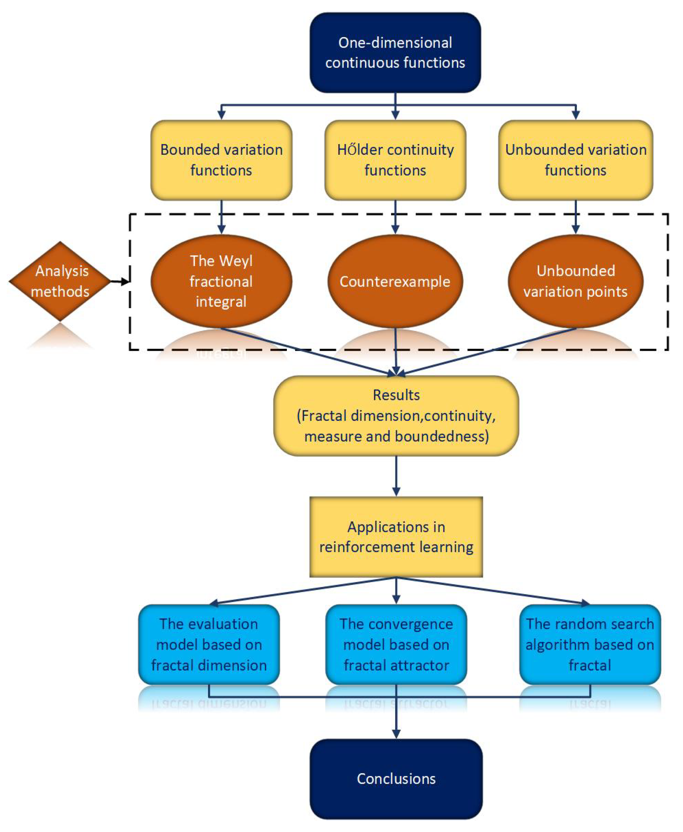
1. Introduction

It is a widely held view that dimensionality is an important indicator to describe functions, but different functions have many disparate internal structures and properties. Traditional topological dimension had not dealt with some characteristics of the intricate functions well. In recent years, there is a growing body of literature that recognises the importance of using fractal dimension instead of topological dimension to describe the functions. The fractal dimension is an extension of the topological dimension. The fractal dimension reflects the effectiveness of the space occupied by the complex sets, and it is a measure of the irregularity of the complex sets. It is cross-combined with the chaos theory of dynamical systems and complements each other. It admits that the part of the world may show similarity with the whole in a certain aspect under certain conditions or processes. The value of the fractal dimension can be not only an integer but also a fraction. So fractal dimension can measure complex sets like the Cantor ternary set. From the point of view of the measure theory, the fractal dimension is the jump point that makes the measure of the set change from infinity to zero. Fractal dimension includes the Hausdorff dimension, the Box dimension and the Packing dimension. Each dimension has a special definition and many calculation methods. The tool for studying fractal dimension is no longer just classic calculus, and a full discussion about the properties of continuous functions lies beyond the scope of classical calculus. Fractional calculus (FC) has gradually become the main method [1,2,3]. Since classical calculus is a special case of fractional calculus [4], many problems that cannot be measured by classical calculus can be solved by fractional calculus, such as studying the properties of continuous functions that are continuous but not differentiable everywhere [5,6]. The most widely used FC is the Riemann-Liuville fractional calculus and the Weyl-Marchaud fractional calculus.

Recent work has established that one-dimensional continuous functions have significant and useful properties [7]. For instance, the Box dimension of bounded variation functions and the functions with Riemann-Liuville fractional calculus are both one. The Box dimension of continuous functions is not less than one. Fractional integral does not increase the dimensionality of the functions, and this special operator makes the fractal dimension have a special linear relationship.

However, there are still some issues that are worth considering and discussing. For example, is the Hausdorff dimension of a continuous function with bounded variation equal to one? What are the Hausdorff dimension and the Box dimension of functions satisfying the H$\ddot{o}$lder condition? Is there a one-dimensional unbounded variation function? Can the function of unbounded variation and bounded variation be mutually converted under special prerequisites? Are there other ways to better explore unbounded variation functions effectively? It is these original questions that promote the emergence of new concepts and many new analytical tools. A few years ago, scholars always used the definition of bounded variation to define the unbounded variation function. The definition is not conducive to exploring the nature of the unbounded variation function. As unbounded variation functions defined by the unbounded variation point directly, a new perspective for studying unbounded variation functions was gradually discovered. At the same time, the relevant conclusions about unbounded variation points have also been rigorously proved. For example, the Box dimension of an unbounded variation function with only an unbounded variation point is one. If this function has self-similarity at the same time, its Hausdorff dimension is also one. A more interesting topic is to investigate the changes between some classic functions and the functions after fractional calculus. These changes usually include fractal dimension [8,9,10], continuity [11,12], boundedness [13,14] and types of fractional calculus [15,16].

After concentrated discussions on some special functions theoretically [17,18], scholars do not have any visual information of the functions [19,20]. The most obvious evidence is the Weierstrass function. Researchers not only know about its functional properties, but also clearly know what its image looks like. Nevertheless, scholars are not very familiar with the image of any one-dimensional continuous functions with an unbounded variation point. Therefore, several attempts have been made to construct the special functions [21], such as one-dimensional continuous functions with finite or infinite unbounded variation points, and unbounded variation functions that satisfy the H$\ddot{o}$lder condition. The construction process of these special functions mainly uses some compression, translation and symmetric transformations. There are also some special unbounded variation functions that are obtained by special operations on the basis of the devil function [22].

So far, there existed many research angles and conclusions on one-dimensional continuous functions and their fractional calculus [23]. In order to have a comprehensive understanding, this paper will systematically sort out the current research results from the perspectives of bounded variation, unbounded variation and the H$\ddot{o}$lder condition. A more detailed analysis of unbounded variation functions through the unbounded variation point will also be elaborated. Combined with the very popular reinforcement learning in machine learning, some very interesting practical applications are predicted. For example, the evaluation model based on the fractal dimension and the random search method based on the fractal structure. The advantage of the fractal evaluation model based on the fractal dimension is that the method based on the local information can evaluate the distance between any two states to the equilibrium state. The distance can speed up the calculation process of algorithms. At the same time, evaluating the current state during the training process can also optimize and improve algorithms reasonably. The fractal random search method also makes full use of the self-similarity to reduce the search time as much as possible on the basis of ensuring the probe of the entire space. Finally, the framework to prove the convergence of reinforcement learning algorithms is introduced using fractal attractors.

The main innovations of this manuscript are as follows. First, the existing conclusions about one-dimensional continuous functions are summarized through three different classification methods, which is helpful to study other complex functions. The second is to introduce the concept of the unbounded variation point to directly study unbounded variation functions. The unbounded variation point can effectively grasp the essence of unbounded variation functions. At the same time, some special unbounded variation functions can be constructed based on the unbounded variation point, and the images of these complex unbounded variation functions can be easily obtained. Third, by combining reinforcement learning and fractal theory, some possible application directions are predicted, and a unique fractal evaluation model is proposed. These results can provide some new ideas for other researchers.

Section 2 mainly recalled some basic concepts, such as the definition of fractal dimension, bounded variation functions, unbounded variation points and fractional calculus. Section 3 mainly discussed the bounded variation function and its fractional calculus. Section 4 focused on the correlation between the continuity of H$\ddot{o}$lder and variation functions. Section 5 primarily explored the unbounded variation function through the unbounded variation point, and gave the construction process of one-dimensional continuous unbounded variation functions. Section 6 forecasted some applications of fractal and fractal functions in reinforcement learning and analyzed the advantages and disadvantages of these methods. The logical structure of this paper is shown in Figure 1.

2. Basic Concepts

Among fractal dimension, the Box dimension is the most widely used. However, some other dimension is still mentioned in some engineering problems, such as the modified Box dimension and the Packing dimension. At the same time, the relationship between these dimension is often analyzed and compared in theoretical research. Most of the definitions are based on measurement theory, and there are also some interrelationships between various dimension. Typical definitions of fractal dimension are as follows.

Definition 1.

([24,25]) Let F be a non-empty bounded subset of $R^n$ and $N_{\delta }\left(F\right)$ be the smallest number of sets of diameter at most δ which can cover F. The lower and upper Box dimension of F respectively are defined as

$${\underline{dim}}_B\left(F\right)=\underset{\delta \to 0}{\underline{lim}}\frac{log{N}_{\delta }\left(F\right)}{-log\delta },$$

(1)

and

$${\overline{dim}}_B\left(F\right)=\overline{\underset{\delta \to 0}{lim}}\frac{log{N}_{\delta }\left(F\right)}{-log\delta }.$$

(2)

If (1) and (2) are equal, the common value is the Box dimension of F:

$${dim}_B\left(F\right)=\underset{\delta \to 0}{lim}\frac{log{N}_{\delta }\left(F\right)}{-log\delta }.$$

If F can be decomposed into a countable number of pieces $F_1,F_2,\cdots$ in such a way that the dimension of the largest piece should be as small as possible. This idea leads to the following modified Box-counting dimension,

$${\underline{dim}}_{MB}\left(F\right)=inf\{\underset{i}{sup}{\underline{dim}}_B{F}_i:F\subset \bigcup _{i=1}^{\infty }{F}_i\},$$

(3)

$${\overline{dim}}_{MB}\left(F\right)=inf\{\underset{i}{sup}{\overline{dim}}_B{F}_i:F\subset \bigcup _{i=1}^{\infty }{F}_i\}.$$

(4)

If (3) and (4) are equal, the common value is the modified Box-counting dimension of F. Let

$${\mathcal{P}}^s\left(F\right)=inf\{\sum _i{\mathcal{P}}_0^s\left(F_i\right):F\subset \bigcup _{i=1}^{\infty }{F}_i\}.$$

It may be shown that ${\mathcal{P}}^s\left(F\right)$ is the s-dimensional Packing measure. The definition of the Packing dimension [26] in the usual way:

$${dim}_{P}F=sup\{s:{\mathcal{P}}^s\left(F\right)=\infty \}=inf\{s:{\mathcal{P}}^s\left(F\right)=0\}.$$

The above dimension is put forward for some specific problems. In the research process, the appropriate fractal dimension should be selected according to the needs. For example, the measurement of the Hausdorff dimension is more accurate and the calculation of the Box dimension is simpler through programs.

The Jordan decomposition theorem is widely applied in the proof process of various problems, and the core concept of the theorem is the function with bounded variation. The definition of the bounded variation function is shown in Definition 2. The unbounded variation function can be defined by the complementary set of bounded variation functions, but this paper will research unbounded variation functions through the unbounded variation point that can be found in Definition 3.

Definition 2.

([27]) Let $f\left(x\right)$ be defined on $I=[0,1]$. A set of points $P=\{x_0,x_1,\cdots ,x_n\}$, satisfying the inequalities $0=x_0<x_1<\cdots <x_{n-1}<x_n=1$, is called a partition. $P=\{x_0,x_1,\cdots ,x_n\}$ is a partition of I and write $△f_k=f\left(x_k\right)-f\left(x_{k-1}\right)$, for $k=1,2,\cdots ,n.$ If there exists a positive number M such that

$$\sum _{k=1}^n|△f_k|\le M,$$

for all partitions of I, $f\left(x\right)$ is said to be of bounded variation on I.

Bounded variation functions have many important properties [28,29]. Such as, a monotonic function is a bounded variation function. The sum, difference, and product of a finite number of bounded variation functions are still the bounded variation function. The absolutely continuous function must be the function of bounded variation.

Definition 3.

(UV point) Let $f\left(x\right)$ be a continuous function on I.

(1) For $p\in (0,1)$. There exists a closed subinterval $Q=[q_1,q_2]$ $(0\le q_1<p<q_2\le 1)$ of I such that the variation of $f\left(x\right)$ on Q is finite, then denote $(p,0)$ as a bounded variation point of $f\left(x\right)$, or $(p,0)$ as an unbounded variation point of $f\left(x\right)$.

(2) For $p=0$ or $p=1$. There is a closed subinterval $Q=[0,q_1]$ $(0<x\le 1)$ or $Q=[q_1,1]$$(0\le q_1<1)$ of I and the variation of $f\left(x\right)$ on Q is finite, then denote $(p,0)$ is a bounded variation point of $f\left(x\right)$, otherwise $(p,0)$ is an unbounded variation point of $f\left(x\right)$.

Due to the complexity of the function structure, the functions of unbounded variation are often non-differentiable functions in the defined interval. The concept of the UV point grasps the essence of unbounded variation functions and transforms the complex structure cleverly. Classical calculus is difficult to analyse the properties of unbounded variation functions, but the properties of some special unbounded variation functions can be investigated by fractional calculus [30,31]. This article mainly utilizes the Riemann-Liouville fractional integral and the Weyl fractional integral [32] to study unbounded variation functions. Their definitions can be found in Definition 4.

Definition 4.

([33,34]) (1) Let $f\left(x\right)\in C_I,\nu >0.$$D^{-\nu }f\left(0\right)=0$ and for $x\in (0,1]$,

$$D^{-\nu }f\left(x\right)=\frac{1}{\Gamma \left(\nu \right)}{\int }_0^x{(x-t)}^{\nu -1}f\left(t\right)dt$$

is the Riemann-Liouville fractional integral of $f\left(x\right)$ of order ν.

(2) Let $f\left(x\right)$ be a continuous function defined on $(-\infty ,+\infty )$ and $0<\nu <1$.

$$W^{-\nu }f\left(x\right)=\frac{1}{\Gamma \left(\nu \right)}{\int }_x^{\infty }{(t-x)}^{\nu -1}f\left(t\right)dt$$

is called as the Weyl fractional integral of $f\left(x\right)$ of order ν.

The abbreviation $C_I$ and $B{V}_I$ will be represented for continuous functions and bounded variation functions defined on I respectively. Denote $G(f,I)$ as the image of $f\left(x\right)$ on I. Denote bounded variation function and unbounded variation function as BVF and UVF respectively. $C_0$ is the Cantor set.

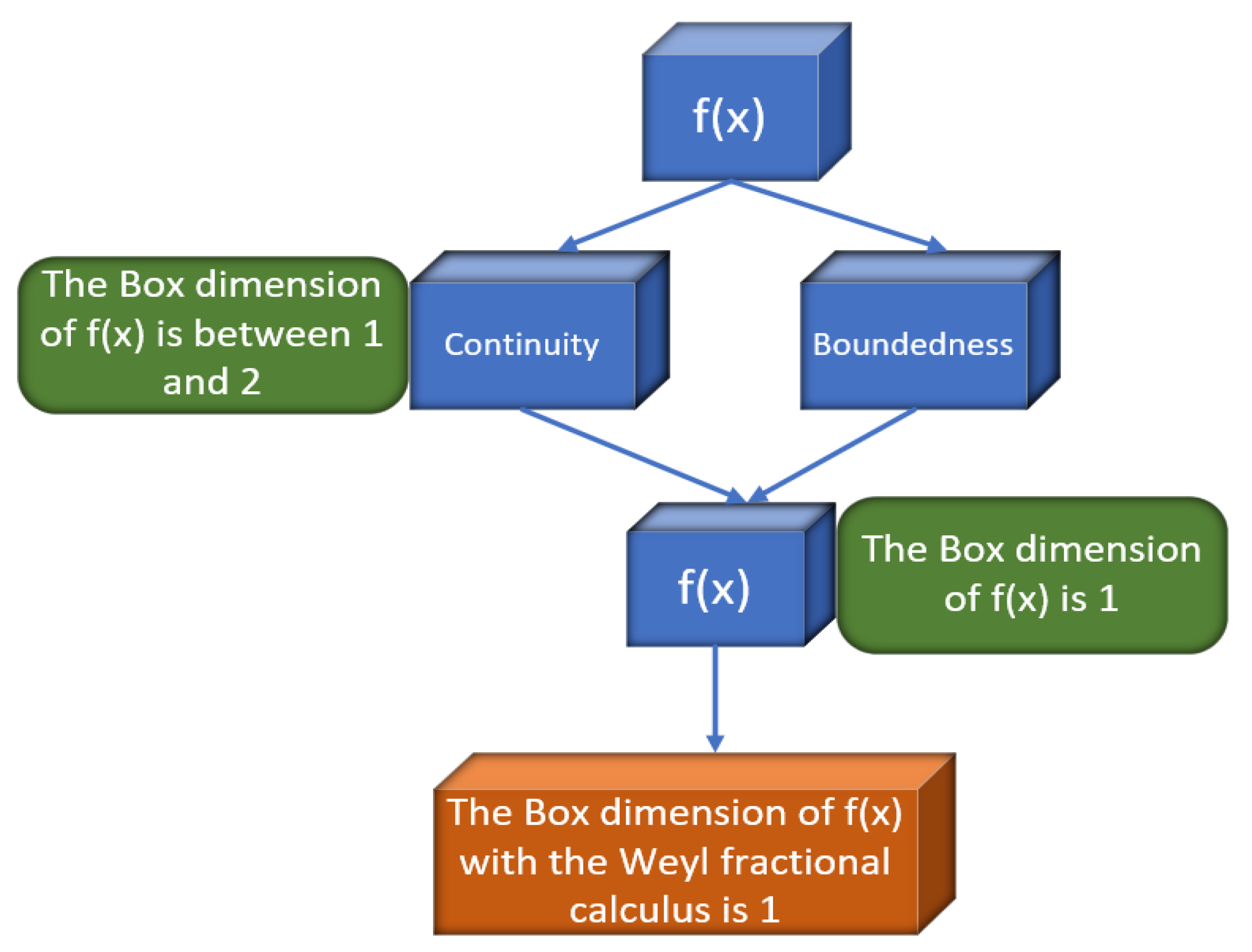
3. Bounded Variation Functions and Their Fractional Integral

The structure of the bounded variation function is not complex. Simple calculations show that its Box dimension is one [35,36]. Furthermore, the bounded variation function after the Weyl fractional integral is still a bounded variation function, so its Box dimension is still one. The relationship between them can be shown in Figure 2.

The proof process of the above related conclusions will be given in detail. First of all, a frequently occurring lemma is necessary to be displayed.

Lemma 1.

Given a function $f\left(x\right)$ and an interval $[a,b]$, $R_f$ is the maximum range of $f\left(x\right)$ over $[a,b]$, i.e.,

$$R_f[a,b]=\underset{a<x,y<b}{sup}|f\left(x\right)-f\left(y\right)|.$$

Let $f\left(x\right)\in C_I\bigcap B{V}_I$. Suppose that $0<\delta <1$ and m be the least integer greater than or equal to ${\delta }^{-1}$. If $N_{\delta }$ is the number of squares of the $\delta -$mesh that intersect $G(f,I)$, then

$${\delta }^{-1}\sum _{i=o}^{m-1}{R}_f[i\delta ,(i+1)\delta ]\le N_{\delta }\le 2m+{\delta }^{-1}\sum _{i=0}^{m-1}{R}_f[i\delta ,(i+1)\delta ].$$

Proof of Lemma 1. 

The number of mesh squares of $\delta$ in the column above the interval $[i\delta ,(i+1\left)\delta \right]$ that intersect $G(f,I)$ belongs to $[R_f[i\delta ,(i+1)\delta ]/\delta ,2+(R_f[i\delta ,(i+1)\delta ]/\delta )]$. By summing all such intervals together, the lemma can be proved. □

Theorem 1.

• (1) If ${\underline{dim}}_{B}G(f,I)\ge 1$ and $f\left(x\right)$ is a continuous function, ${\overline{dim}}_{B}G(f,I)\le 2$.
• (2) If $f\left(x\right)\in C_I\bigcap B{V}_I$, ${dim}_{B}G(f,I)=1$.

Proof of Theorem 1. 

By using Definition 1,

$${\underline{dim}}_{B}G(f,I)\ge \underset{\delta \to 0}{\underline{lim}}\frac{log\frac{C}{\delta }}{-log\delta }=1,{\overline{dim}}_{B}G(f,I)\le \underset{\delta \to 0}{\overline{lim}}\frac{log\frac{C}{{\delta }^2}}{-log\delta }=2.$$

Let ${\left\{x_i\right\}}_{i=1}^n$ be arbitrary points satisfying $0=x_0<x_1<x_2<\cdots <x_n=1$, then

$$\underset{(x_0,x_1,\cdots ,x_n)}{sup}\sum _{k=1}^n|f\left(x_k\right)-f\left(x_{k-1}\right)|<C.$$

Let m be the least integer greater than or equal to $\frac{1}{\delta }$. $N_{\delta }$ is the number of squares of the $\delta -$mesh that intersect $G(f,I)$. Combining Lemma 1,

$$N_{\delta }\le 2m+{\delta }^{-1}\sum _{i=1}^m{R}_f[(i-1)\delta ,i\delta ].$$

For $1\le i\le m-1$ and $x_{i,0}=i\delta$, $x_{i,3}=(i+1)\delta$, $x_{i,1},x_{i,2}\in (i\delta ,(i+1)\delta ),$

$$R_f[i\delta ,(i+1)\delta ]\le \underset{x_{i,0}<x_{i,1}<x_{i,2}<x_{i,3}}{sup}\sum _{k=1}^3|f(x_i,k)-f(x_i,k-1)|.$$

There exists a positive constant C such that $N_{\delta }\le C{\delta }^{-1}$ and

$${\overline{dim}}_{B}G(f,I)\le 1,0<v<1.$$

Simultaneously, the topolopy dimension of a continuous function $f\left(x\right)$ is no less than 1,

$${\underline{dim}}_{B}G(f,I)\ge 1,0<v<1.$$

Thus, ${dim}_{B}G(f,I)=1$. □

If non-negative constants C and $\alpha$ can be found to formula the following inequation

$$|f\left(x\right)-f\left(y\right)|\le {C|x-y|}^{\alpha },$$

$f\left(x\right)$ is a H$\ddot{o}$lder continuous function [37]. When $\alpha =1$, $f\left(x\right)$ is a Lipschitz continuous function. Throughout this paper, the term $f\left(x\right)\in LipC$ means that $f\left(x\right)$ is a Lipschitz continuous function on I and the Lipschitz constant is C.

Corollary 1.

If $f\left(x\right)\in LipC$, then ${dim}_{B}G(f,I)=1$.

Proof of Corollary 1. 

$f\left(x\right)\in LipC$, $\forall x,y\in I$,

$$\mid f\left(x\right)-f\left(y\right)\mid \le C\mid x-y\mid .$$

Let ${\left\{x_i\right\}}_{i=1}^n$ be arbitrary points satisfying $0=x_0<x_1<x_2<\cdots <x_n=1$. Since

$$\underset{(x_0,x_1,...,x_n)}{sup}\sum _{k=1}^n|f\left(x_k\right)-f\left(x_{k-1}\right)|\le C\sum _{k=1}^n|x_k-x_{k-1}|\le C,$$

$f\left(x\right)\in B{V}_I$ and ${dim}_{B}G(f,I)=1$. □

Corollary 1 shows that a function that satisfies the Lipschitz condition must be a BVF. However, a function that satisfies the H$\ddot{o}$lder condition is not necessarily a BVF [38,39]. The counter-example is as follows:

$$f\left(x\right)=\left\{\begin{array}{cc}-1/\mathrm{l}\mathrm{n}\mathrm{x},\hfill & 0<x\le 0.5,\hfill \\ 0,\hfill & x=0.\hfill \end{array}\right.$$

Obviously, since this function is monotonically increasing in $[0,0.5]$, it is a BVF. But for any $\alpha >0$, this function does not satisfy the H$\ddot{o}$lder condition of order $\alpha$.

Theorem 2.

If $f\left(x\right)\in C_I\bigcap B{V}_I$, ${dim}_{B}G(W^{-v}f,I)=1$.

Proof of Theorem 2. 

Since $f\left(x\right)\in C_I$ and $f\left(x\right)$ is of bounded variation on I, $f\left(x\right)$ can be replaced with the difference of two monotone increasing and continuous functions $g_1\left(x\right)$ and $g_2\left(x\right)$ by the Jordan decomposition theorem, $f\left(x\right)=g_1\left(x\right)-g_2\left(x\right)$, where $g_1\left(x\right)=h_1\left(x\right)-c$, $g_2\left(x\right)=h_2\left(x\right)-c$, $h_1\left(x\right)=h_2\left(x\right)=c$ on $[1,+\infty )$. Then $h_1\left(x\right)$ and $h_2\left(x\right)$ are also monotone increasing and continuous functions.

(1) If $f\left(0\right)\ge 0$, let $g_1\left(0\right)\ge 0$ and $g_2\left(0\right)=0$. By Definition 4,

$$G_1\left(x\right)=W^{-v}{g}_1\left(x\right)=\frac{1}{\Gamma \left(v\right)}{\int }_x^{\infty }\frac{h_1\left(t\right)-c}{{(t-x)}^{1-v}}dt,0<v<1,$$

$G_1\left(x\right)$ still is a continuous function on I when $g_1\left(x\right)$ is a continuous function. Let $0\le x_1\le x_2\le 1$ and $0<v<1$,

$$\begin{array}{cc}\hfill & G_1\left(x_2\right)-G_1\left(x_1\right)\hfill \\ \hfill =& \frac{1}{\Gamma \left(v\right)}{\int }_{x_2}^{\infty }{(t-x_2)}^{v-1}(h_1\left(t\right)-c)dt-\frac{1}{\Gamma \left(v\right)}{\int }_{x_1}^{\infty }{(t-x_1)}^{v-1}(h_1\left(t\right)-c)dt\hfill \\ \hfill =& \frac{1}{\Gamma \left(v\right)}{\int }_{x_2}^1{(t-x_2)}^{v-1}(h_1\left(t\right)-c)dt-\frac{1}{\Gamma \left(v\right)}{\int }_{x_1}^1{(t-x_1)}^{v-1}(h_1\left(t\right)-c)dt\hfill \\ \hfill =& \frac{1}{\Gamma \left(v\right)}({\int }_{x_2}^1{(t-x_2)}^{v-1}{h}_1\left(t\right)dt-{\int }_{x_1}^1{(t-x_1)}^{v-1}{h}_1\left(t\right)dt)\hfill \\ \hfill & +\frac{1}{\Gamma \left(v\right)}({\int }_{x_1}^1{(t-x_1)}^{v-1}cdt-{\int }_{x_2}^1{(t-x_2)}^{v-1}cdt)\hfill \\ \hfill =& \frac{1}{\Gamma \left(v\right)}{\int }_{x_1}^{1-x_2+x_1}{(t-x_1)}^{v-1}(h_1(t-x_1+x_2)-h_1\left(t\right))dt\hfill \\ \hfill & +\frac{1}{\Gamma \left(v\right)}{\int }_{1+x_1-x_2}^1{(t-x_1)}^{v-1}(c-h_1\left(t\right))dt\hfill \\ \hfill \ge & 0.\hfill \end{array}$$

Thus, $G_1\left(x\right)$ still is a monotone increasing and continuous function on I. If

$$G_2\left(x\right)=W^{-v}{g}_2\left(x\right)=\frac{1}{\Gamma \left(v\right)}{\int }_x^{\infty }\frac{h_2\left(t\right)-c}{{(t-x)}^{1-v}}dt,0<v<1,$$

$G_2\left(x\right)$ is also a monotone increasing and continuous function on I.

(2) If $f\left(0\right)<0$, let $g_1\left(x\right)=0$ and $g_2\left(x\right)>0$. Using a similar way, both $W^{-v}{g}_1\left(x\right)$ and $W^{-v}{g}_2\left(x\right)$ are monotone increasing and continuous functions on I. So $W^{-v}f\left(x\right)$ still is a BVF on I and

$${dim}_{B}G(W^{-v}f,I)=1.$$

□

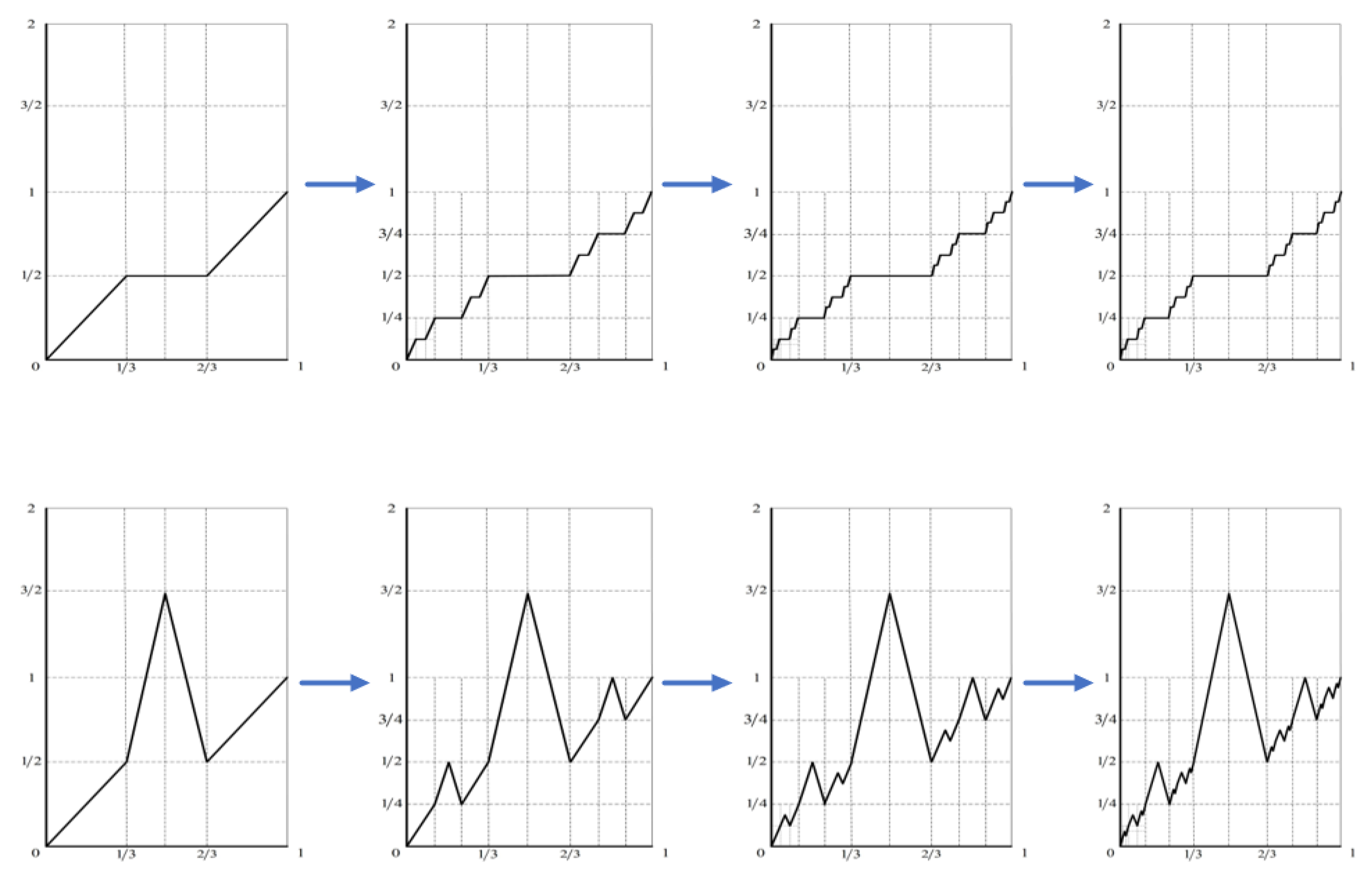
4. Unbounded Variation Functions (UVFs)

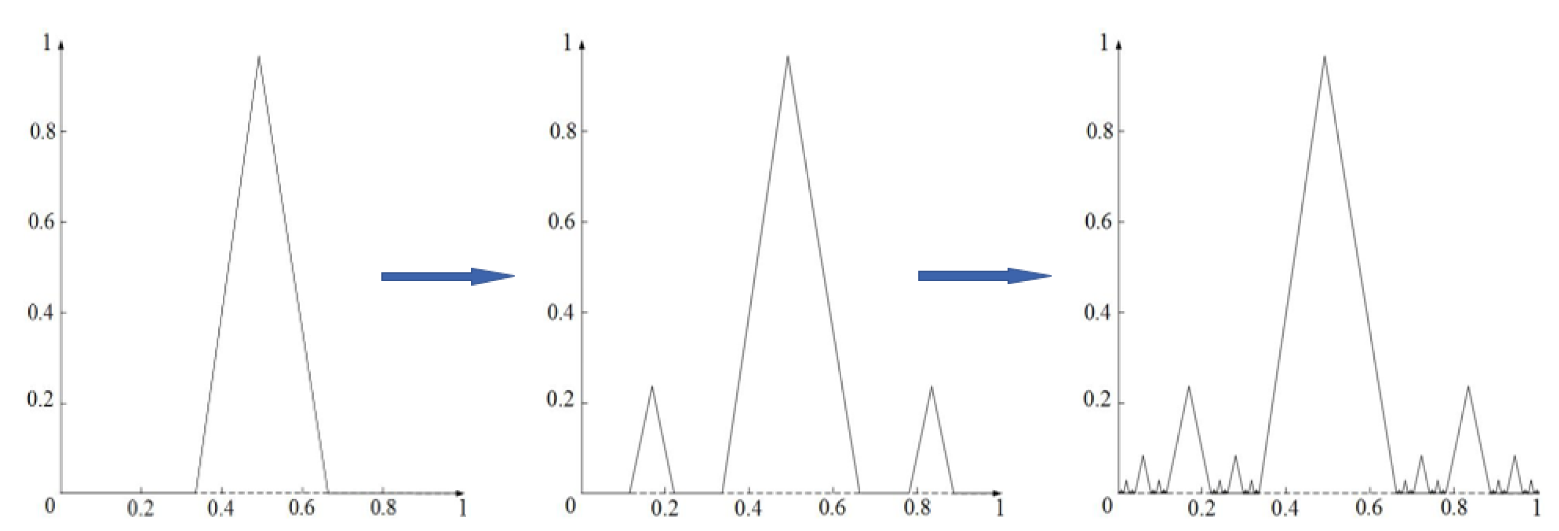
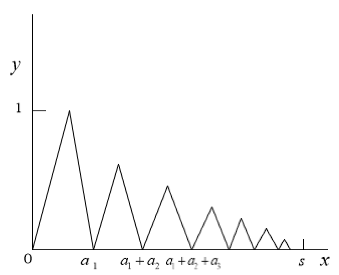
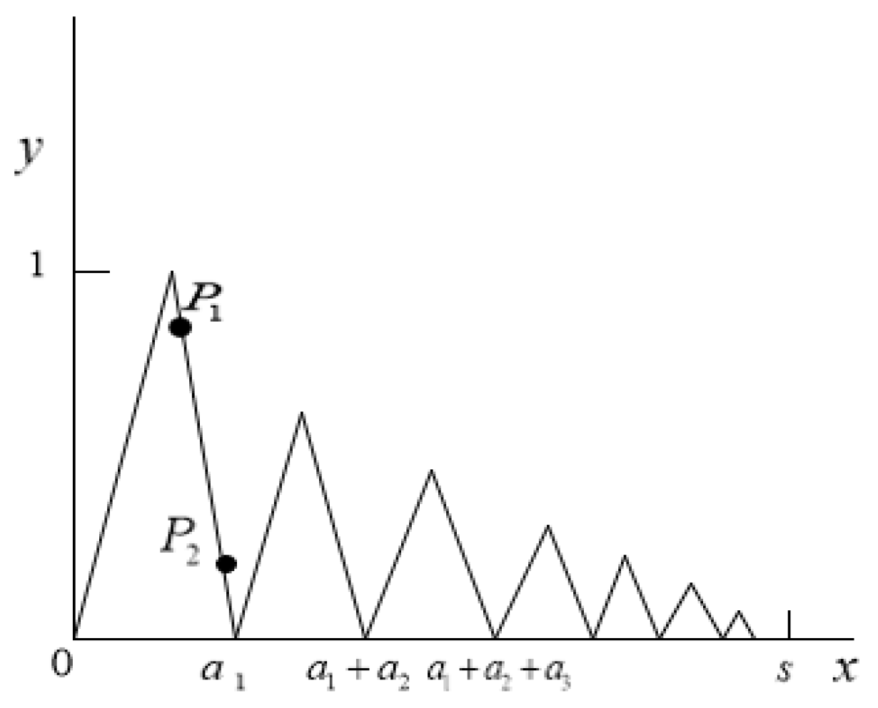
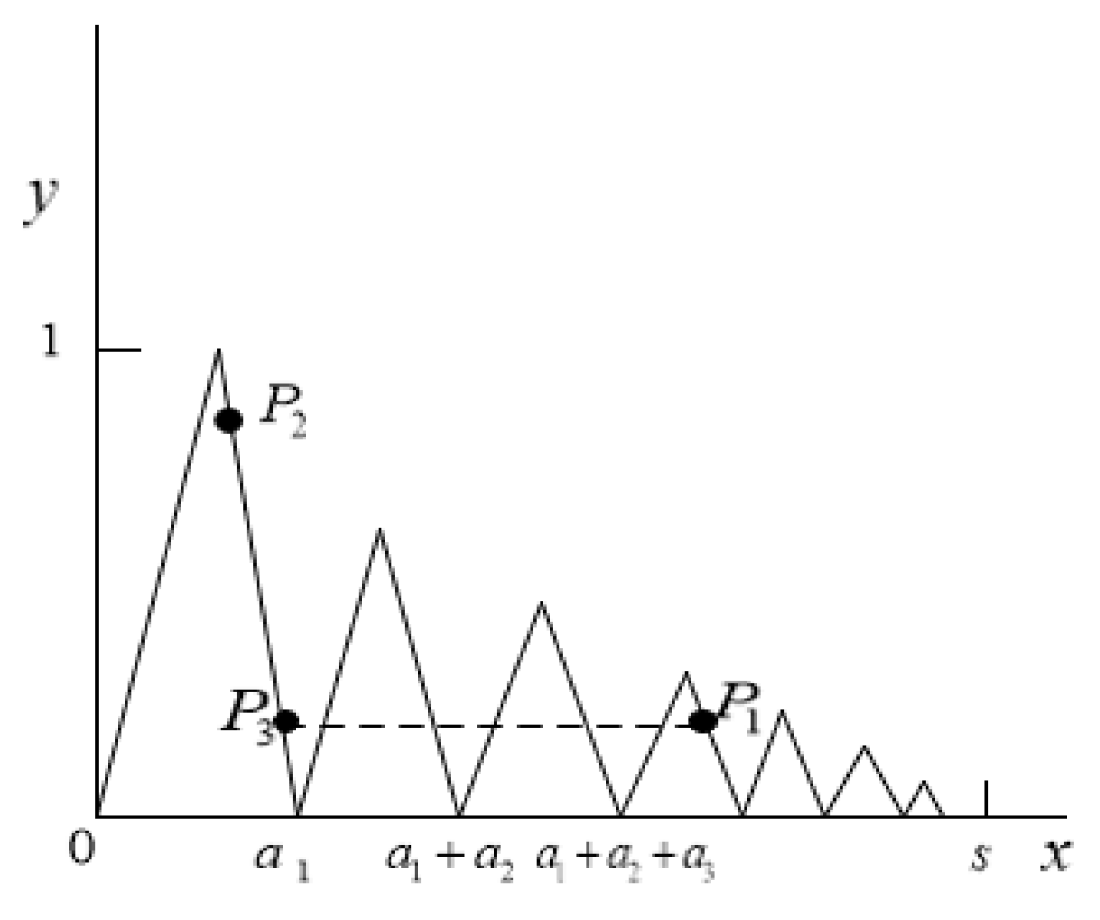
4.1. A Special UVF

The construction process of the devil stair function $d\left(x\right)$ will be elaborated firstly. Then, a peculiar continuous function $D\left(x\right)$ of unbounded variation on I will be constructed on the basis of $d\left(x\right)$.

If $x\in (\frac{1}{3},\frac{2}{3})$, $d_1\left(x\right)=\frac{1}{2}$. Let $d_1\left(0\right)=0$ and $d_1\left(1\right)=1$. $d_1\left(x\right)$ can be exhibited on I by connecting $d_1\left(0\right)$, $d_1\left(\frac{1}{3}\right)$, $d_1\left(\frac{2}{3}\right)$ and $d_1\left(1\right)$ with line segments.

If $x\in (\frac{1}{9},\frac{2}{9})$, $d_2\left(x\right)=\frac{1}{4}$. If $x\in (\frac{7}{9},\frac{8}{9})$, $d_2\left(x\right)=\frac{3}{4}$. Connecting $d_1\left(0\right)$, $d_2\left(\frac{1}{9}\right)$, $d_2\left(\frac{2}{9}\right)$, $d_1\left(\frac{1}{3}\right)$, $d_1\left(\frac{2}{3}\right)$, $d_2\left(\frac{7}{9}\right)$, $d_2\left(\frac{8}{9}\right)$ and $d_1\left(1\right)$ with line segments to form $d_2\left(x\right)$ on I.

By induction, $d_n\left(x\right)(n\ge 3)$ can be constructed. Let $d\left(x\right)={lim}_{n\to \infty }{d}_n\left(x\right).$

The construction of $D_1\left(x\right)$ is based on $d_1\left(x\right)$ with two more line segments whose length are 1. The line segments and the part of $d_1\left(x\right)$, $x\in (\frac{1}{3},\frac{2}{3})$ make up an isosceles triangle. In $D_1\left(x\right)$, the triangle is shown without the base line.

The construction of $D_2\left(x\right)$ is based on $d_2\left(x\right)$ and $D_1\left(x\right)$. Simultaneously for $x\in (0,\frac{1}{3})$ or $x\in (\frac{1}{3},\frac{2}{3})$, using similar ways to construct $D_2\left(x\right)$ like as $d_1\left(x\right)\to D_1\left(x\right)$. However, the length of line segments added is $\frac{1/2}{2^1}$.

The construction of $D_3\left(x\right)$ is based on $d_3\left(x\right)$ and $D_2\left(x\right)$. Simultaneously for $x\in (0,\frac{1}{9})$, $x\in (\frac{2}{9},\frac{1}{3})$, $x\in (\frac{2}{3},\frac{7}{9})$, or $x\in (\frac{8}{9},1)$, using similar steps to construct $D_3\left(x\right)$ like as $d_1\left(x\right)\to D_1\left(x\right)$. The process of constructing is similar, the only difference is the length of line segments added is $\frac{1/3}{2^2}$.

By induction, the construction of $D_n\left(x\right)$ is based on $d_n\left(x\right)$ and $D_{n-1}\left(x\right)$. The length of line segments is $\frac{1/n}{2^{n-1}}$. Then, $D\left(x\right)={lim}_{n\to \infty }{D}_n\left(x\right).$ Images of $d\left(x\right)$ and $D\left(x\right)$ are given as follows Figure 3.

Combining the construction process of $D\left(x\right)$, properties of the function will be investigated.

Property 1.

The length of $G(D,I)$ is infinite on I. The lebesgue measure of differentiable points on I is one.

Proof of Property 1.

Length of $G(D,I)$ is no less than

$$1·2·1+2·2·\frac{1/2}{2}+4·2·\frac{1/3}{4}+\cdots +2^{n-1}·2·\frac{1/n}{2^{n-1}}+\cdots =2\sum _{n=1}^{\infty }\frac{1}{n}=\infty .$$

Thus, the length of $G(D,I)$ is infinite on I. Let A be the set of differentiable points of $D\left(x\right)$ on I.

$$m\left(A\right)=\frac{1}{3}+2·\frac{1}{9}+4·\frac{1}{27}+\cdots +2^{n-1}·\frac{1}{3^n}+\cdots =1.$$

Denote B as the set of non-differentiable points of $D\left(x\right)$ on I, then

$$m\left(B\right)=1-1=0.$$

□

Property 2.

The Box dimension of $D\left(x\right)$ is one and $D\left(x\right)$ has uncountable unbounded variation points on I.

Proof of Property 2.

Since $D\left(x\right)$ is a continuous function, ${\underline{dim}}_{B}G(D,I)\ge 1$. Let $0<\delta <1$, $\frac{1}{\delta }\le n\le 1+\frac{1}{\delta }$. The number of squares of the $\delta -$mesh that intersect $G(D,I)$ are less than

$$2n+\frac{1}{\delta }\sum _{i=1}^n\frac{1}{i}+2\frac{1}{\delta }.$$

Thus,

$$\begin{array}{cc}\hfill {\overline{dim}}_{B}G(D,I)& \le \overline{\underset{\delta \to 0}{lim}}\frac{log[2n+\frac{1}{\delta }{\displaystyle \sum _{i=1}^n}\frac{1}{i}+2\frac{1}{\delta }]}{-log\delta }\hfill \\ \hfill & \le \overline{\underset{\delta \to 0}{lim}}\frac{log[2n+2{\delta }^{-1}(log(n+1)+1)]}{-log\delta }\hfill \\ \hfill & \le 1.\hfill \end{array}$$

Further analysis showed that ${dim}_{B}G(D,I)=1$.

If $\forall x\in C_0$, a positive number $N_0$ will be found such that variation of any subinterval $I_x$ containing x of I is at least

$$\begin{array}{cc}\hfill & \frac{1}{2^{N_0}}\frac{1}{N_0}+2\frac{1}{2^{N_0+1}}\frac{1}{N_0+1}+2^2\frac{1}{2^{N_0+2}}\frac{1}{N_0+2}+\cdots \hfill \\ \hfill & =\frac{1}{2^{N_0}}\sum _{n=1}^{\infty }\frac{1}{N_0+n-1}\hfill \\ \hfill & =\frac{1}{2^{N_0}}(\sum _{n=1}^{\infty }\frac{1}{n}-\sum _{n=1}^{N_0-1}\frac{1}{n})\hfill \\ \hfill & =\infty .\hfill \end{array}$$

Thus, $(x,0)$ is an unbounded variation point of $D\left(x\right)$ on I. Since the arbitrariness of x, the number of unbounded variation points of $D\left(x\right)$ on I is uncountable. □

Now, the construction of $H\left(x\right)$ that contains uncountable UV points will be displayed. Divided I into three equal intervals,

$$I_{1,1}=[0,\frac{1}{3}],I_{1,2}=[\frac{1}{3},\frac{2}{3}],I_{1,3}=[\frac{2}{3},1].$$

Two line segments are added such that constituting an isosceles triangle with $I_{1,2}$ and the length of the segment is 1, Then $I_{1,2}$ will be removed. $I_{1,1}$ and $I_{1,3}$ are divided into three equal intervals respectively,

$$\begin{array}{c}\hfill I_{1,1}=I_{2,1}\bigcup I_{2,2}\bigcup I_{2,3},\\ \hfill I_{1,3}=I_{2,4}\bigcup I_{2,5}\bigcup I_{2,6}.\end{array}$$

Four line segments are added such that constituting an isosceles triangle with $I_{2,2}$ and $I_{2,5}$. The length of the segment is $\frac{1}{4}$. Furthermore, delete $I_{2,2}$ and $I_{2,5}$. Similar way can get $H_3$ and $H_4$. $H_n$ can be got From $H_{n-1}$. By dividing

$$I_{n-1,1},I_{n-1,3},I_{n-1,4},I_{n-1,6},\cdots ,I_{n-1,3·2^{n-2}-1},I_{n-1,3·2^{n-2}}$$

into three equal intervals respectively,

$$\begin{array}{cc}\hfill I_{n-1,1}& =I_{n,1}\bigcup I_{n,2}\bigcup I_{n,3},\hfill \\ \hfill I_{n-1,3·2^{n-2}}& =I_{n,3·2^{n-1}-2}\bigcup I_{n,3·2^{n-1}-1}\bigcup I_{n,3·2^{n-1}}.\hfill \end{array}$$

$2^n$ line segments are added such that constituting an isosceles triangle with

$$I_{n-1,2},I_{n-1,5},\cdots ,I_{n-1,3·2^{n-2}-1}.$$

The length of the segment is $\frac{1}{n·2^{n-1}}$. Then delete $I_{n,2}$, $I_{n,5}$,⋯, $I_{n,3·2^{n-1}-1}$. The image of $H\left(x\right)$ is Figure 4.

Obviously, $H\left(x\right)$ is a continuous function. Firstly, the length of $H\left(x\right)$ on I is ${\displaystyle \sum _{n=1}^{\infty }}\frac{1}{n}=\infty$, the variation of $H\left(x\right)$ on I is infinite. Secondly, the number of $\delta -$mesh squares that intersect $G(H,I)$ is at most ${\delta }^{-1}{\displaystyle \sum _{n=1}^{\infty }}\frac{1}{n}+2{\delta }^{-1}$ and

$${dim}_{B}G(H,I)=\underset{\delta \to 0}{lim}\frac{log({\delta }^{-1}{\displaystyle \sum _{n=1}^{\infty }}\frac{1}{n}+2{\delta }^{-1})}{-log\delta }=1.$$

Finally, $\forall x_0\in C_0\cup [a,b]$, the variation of $H\left(x\right)$ on $[a,b]$ is ${\displaystyle \sum _{n=N_0}^{\infty }}\frac{1}{N_0{2}^{N_0-1}}\frac{1}{n}=\infty$, where $N_0$ is a positive integer. So $H\left(x\right)$ contains uncountable UV points.

The function that satisfies the Lipschitz condition must be a BVF, but the function that satisfies the H$\ddot{o}$lder condition is not necessarily a BVF [40,41]. The following two special functions are just the best evidence for the above conclusion.

4.2. UVF Satisfying the H$\ddot{o}$lder Condition of Order $\alpha (0<\alpha <1)$

Let $A_n=a_1+a_2+\cdots +a_n+\cdots$ be the convergence series of positive terms and any of terms is monotonically decreasing. The sum of $A_n$ is s and the construction process of the function $f_{\alpha }\left(x\right)$ on $[0,s]$ is as follows:

$$\begin{array}{cc}\hfill f\left(x\right)& =0,x\in \{0,a_1,a_1+a_2,a_1+a_2+a_3\};\hfill \\ \hfill f\left(x\right)& =\frac{1}{n},x\in \{a_1+a_2+\cdots +a_{n-1}+\frac{a_n}{2}(n=1,2,\cdots )\};\hfill \\ \hfill f\left(s\right)& =0.\hfill \end{array}$$

$f_{\alpha }\left(x\right)$ is linear in the following intervals, such as $[a_1+\cdots +a_{n-1},a_1+\cdots +a_{n-1}+\frac{a_n}{2}]$, $[a_1+\cdots +a_{n-1}+\frac{a_n}{2},a_1+\cdots +a_{n-1}+a_n]$, $n=1,2,\cdots$. The specific image of $f_{\alpha }\left(x\right)$ is as follows Figure 5.

Theorem 3.

$f_{\alpha }\left(x\right)$ is a continuous function on $[0,s](0<s\le 1)$ and the total variation of $f_{\alpha }\left(x\right)$ in the interval $[0,s]$ is infinite.

Proof of Theorem 3.

From the specific construction process of $f_{\alpha }\left(x\right)$, $f_{\alpha }\left(x\right)$ is a continuous function on $[0,s]$ obviously. The proof of its total variation is infinite will be given next. Consider the following partition: $0<\frac{a_1}{2}<a_1<a_1+\frac{a_2}{2}<+a_1+a_2<a_1+a_2+\frac{a_3}{2}<a_1+a_2+a_3<\cdots <a_1+a_2+\cdots +a_k$. Then,

$$\begin{array}{cc}\hfill V_0^s\left(f\left(x\right)\right)=& |f(\frac{a_1}{2})-f\left(0\right)|+|f\left(a_1\right)-f(\frac{a_1}{2})|+|f(a_1+\frac{a_1}{2})-f\left(a_1\right)|\hfill \\ \hfill & +\cdots +|f(a_1+a_2+\cdots +a_k)-f(a_1+a_2+\cdots +a_{k-1}+\frac{a_k}{2})|\hfill \\ \hfill & +|f\left(s\right)-f(a_1+a_2+\cdots +a_k)|\hfill \\ \hfill =& 1+1+\frac{1}{2}+\frac{1}{2}+\cdots +\frac{1}{k}+\frac{1}{k}\hfill \\ \hfill =& +\infty .\hfill \end{array}$$

The conclusion is $\underset{k\to +\infty }{lim}{V}_0^s\left(f\left(x\right)\right)=+\infty$. Thus, $f_{\alpha }\left(x\right)$ is an UVF on $[0,s]$. □

Theorem 4.

$f_{\alpha }\left(x\right)$ satisfies the H$\ddot{o}$lder condition of a given order $\alpha (0<\alpha <1)$.

Proof of Theorem 4.

Case one: two points $P_1(x_1,y_1)$, $P_2(x_2,y_2)$ on the interval are selected arbitrarily, but the two points are in the same linear interval, $a_1+\cdots +a_{n-1}\le x_1<x_2\le a_1+\cdots +a_{n-1}+\frac{a_n}{2}$. Then the specific image of Case one is as follows Figure 6.

$$\begin{array}{cc}\hfill |y_2-y_1|& =\frac{2}{n{a}_n}|x_2-x_1|=\frac{2|x_2-x_1{|}^{1-\alpha }}{n{a}_n}{|x_2-x_1|}^{\alpha }\hfill \\ \hfill & <\frac{2a_n^{1-\alpha }}{n{a}_n}{|x_2-x_1|}^{\alpha }\hfill \\ \hfill & =\frac{2}{n{a}_n^{\alpha }}{|x_2-x_1|}^{\alpha }.\hfill \end{array}$$

Therefore, it is significant to select the appropriate sequence $a_n$ to make $\frac{2}{n{a}_n^{\alpha }}$ bounded. a sequence that satisfies the above formula can be found easily, such as $a_n=n^{\frac{-1}{\alpha }}$.

Case two: If the two points $P_1(x_1,y_1)$, $P_2(x_2,y_2)$ are not in the same linear interval, moving $P_1$ to $P_3(x_3,y_3)$ through translation transformation. Then the specific image of Case two is as follows Figure 7.

Combined with the proof of Case one, $|y_2-y_1|=|y_2-y_3|\le C|x_2-x_3{|}^{\alpha }$.

□

Since $f_{\alpha }\left(x\right)$ is a continuous function, the lower Box dimension of $f_{\alpha }\left(x\right)$ is greater than or equal to 1. The number of $\delta -$mesh squares that intersect $G(f_{\alpha },[0,s])$ is at most ${\delta }^{-1}{\displaystyle \sum _{n=1}^{\infty }}\frac{1}{n}+2{\delta }^{-1}$,

$${dim}_{B}G(f_{\alpha },[0,s])=\underset{\delta \to 0}{lim}\frac{log({\delta }^{-1}{\displaystyle \sum _{n=1}^{\infty }}\frac{1}{n}+2{\delta }^{-1})}{-log\delta }=1.$$

4.3. UVF Not Satisfying the H$\ddot{o}$lder Condition of Any Order $\alpha (\alpha >0)$

An UVF $g\left(x\right)$ that does not satisfy the H$\ddot{o}$lder condition of any order $\alpha (\alpha >0)$ on the basis of $f_{\alpha }\left(x\right)$ will be constructed. Since $f_{\alpha }\left(x\right)$ satisfies the H$\ddot{o}$lder condition of order $\alpha (0<\alpha <1)$ on $[0,s]$, for ${\alpha }^{*}>\alpha$, $x=a_1+a_2+\cdots +a_{n-1}+\frac{a_n}{2}$, $y=a_1+a_2+\cdots +a_{n-1}+a_n$,

$$\begin{array}{cc}\hfill \underset{n\to +\infty }{lim}\frac{f\left(y\right)-f\left(x\right)}{{|y-x|}^{{\alpha }^{*}}}& =\frac{\frac{1}{n}}{{\left(\frac{a_n}{2}\right)}^{{\alpha }^{*}}}=\frac{\frac{1}{n}}{{(\frac{1}{2n^{\frac{1}{\alpha }}})}^{{\alpha }^{*}}}=2^{{\alpha }^{*}}{n}^{\frac{{\alpha }^{*}}{\alpha }-1}=+\infty .\hfill \end{array}$$

Thus, $f_{\alpha }\left(x\right)$ does not satisfy the H$\ddot{o}$lder condition of any order ${\alpha }^{*}({\alpha }^{*}>\alpha )$ on $[0,s]$.

Denote ${\sigma }_n={\displaystyle \sum _{k=1}^{\infty }}\frac{1}{k^n}$ and divide the interval I as follows,

$$0={\beta }_2<{\beta }_3<{\beta }_4<\cdots <{\beta }_n<\cdots ({\beta }_n\to 1,n\to +\infty ).$$

(1) If n is an even number, $g\left(x\right)$ can be obtained by compressing $f_{\frac{1}{n}}\left(x\right)$ by n times on the ordinate, compressing by $\frac{{\sigma }_n}{{\beta }_{n+1}-{\beta }_n}$ times on the abscissa and moving ${\beta }_n$ to the right along the abscissa,

$$g\left(x\right)=\frac{1}{n}{f}_{\frac{1}{n}}[\frac{{\sigma }_n(x-{\beta }_n)}{{\beta }_{n+1}-{\beta }_n}].$$

(2) If n an is odd number,

$$g\left(x\right)=\frac{1}{n}{f}_{\frac{1}{n}}[\frac{{\sigma }_n({\beta }_{n+1}-x)}{{\beta }_{n+1}-{\beta }_n}].$$

In addition to the above construction process, an additional supplementary definition $f\left(1\right)=0$ is reasonable. The specific image of $g\left(x\right)$ is as follows Figure 8.

From the construction process of $g\left(x\right)$, $g\left(x\right)$ is defined everywhere on the interval I and $g\left(x\right)$ is a continuous function. Through similar calculation, it can be known that the total variation of this function is also infinite. $g\left(x\right)$ is also an UVF.

However, for interval $[{\beta }_n,{\beta }_{n+1}]$, $g\left(x\right)$ satisfies the H$\ddot{o}$lder condition of order $\frac{1}{n}$ and does not satisfy the H$\ddot{o}$lder condition of order $\frac{1}{n-1}$. Therefore, the function $g\left(x\right)$ does not satisfy the H$\ddot{o}$lder condition of any order $\alpha (\alpha >0)$. Since $g\left(x\right)$ is a continuous function, the Box dimension of $g\left(x\right)$ is more than one.

4.4. UVF Contained Finite UV Points

The introduction of the unbounded variation points gives a new way to study unbounded variation functions [42]. Many conclusions about unbounded variation functions can be obtained by analyzing the number and location of unbounded variation points. At the same time, if the function has self-similarity, some remarkable conclusions can be strictly demonstrated, such as Corollary 2 and Theorem 8.

Lemma 2.

([24]) If $F\subset R^n$, then ${dim}_{P}F={\overline{dim}}_{MB}F$.

Researchers have established the following relation for $F\subset R^n$:

$${dim}_{H}F\le {\underline{dim}}_{MB}F\le {\overline{dim}}_{MB}F={dim}_{P}F\le {\overline{dim}}_{B}F.$$

Theorem 5.

If $f\left(x\right)$ is a continuous function on I and $(1,0)$ is the only UV point of $f\left(x\right)$, then

$${dim}_{H}G(f,I)={dim}_{P}G(f,I)={dim}_{MB}G(f,I)=1.$$

Proof of Theorem 5.

Since $f\left(x\right)$ is a continuous function on I,

$$1\le {dim}_{H}G(f,I)\le {\underline{dim}}_{B}G(f,I).$$

$\forall \delta >0$, $I=\left({\displaystyle \bigcup _{i=1}^{\infty }}{E}_i\right)\bigcup [1-\delta ,1]$, where $E_i$ are subsets of I.

$${dim}_{H}G(f,[1-\delta ,1])\le {\overline{dim}}_{B}G(f,[1-\delta ,1])\le \underset{\delta \to 0}{\overline{lim}}\frac{log\frac{M}{\delta }}{-log\delta }=1,$$

where M is a positive constant.

$${\overline{dim}}_{MB}G(f,I)=inf\{\underset{\delta }{sup}{\overline{dim}}_{B}G(f,(\bigcup _{i=1}^{\infty }{E}_i)\bigcup [1-\delta ,1])\}=1.$$

Thus,

$$1\le {dim}_{H}G(f,I)\le {\overline{dim}}_{MB}G(f,I)=1.$$

It is already becoming apparent that

$${dim}_{H}G(f,I)={dim}_{P}G(f,I)={dim}_{MB}G(f,I)=1.$$

□

Theorem 6.

If $f\left(x\right)$ is a continuous function containing at most finite UV points on I, then

$${dim}_{H}G(f,I)={dim}_{P}G(f,I)={dim}_{MB}G(f,I)=1.$$

Proof of Theorem 6.

Let $x_1<x_2<\cdots <x_n$ be UV points of $f\left(x\right)$, n disjoint intervals $[a_i,x_i]\subset I$ can be found, where $i=1,2,\cdots ,n$. Denote $A={\displaystyle \bigcup _{i=1}^n}[a_i,x_i]$. By Lemma 2,

$${dim}_{H}G(f,[a_i,x_i])={dim}_{P}G(f,[a_i,x_i])={dim}_{MB}G(f,[a_i,x_i])=1.$$

Since the Hausdorff dimension has the property of countable stability,

$$\begin{array}{cc}\hfill {dim}_{H}G(f,I)& ={dim}_{H}G(f,A\bigcup (I\backslash A))\hfill \\ \hfill & =max\{{dim}_{H}G(f,A),{dim}_{H}G(f,I\backslash A)\}\hfill \\ \hfill & =1.\hfill \end{array}$$

Given $\epsilon =\underset{1\le i<j\le n}{min}|x_i-x_j|$, $C_i=[a_i-\frac{\epsilon }{2},a_i+\frac{\epsilon }{2}]$, $C_{n+1}=I\backslash \left({\displaystyle \bigcup _{i=1}^n}{C}_i\right)$.

$${\overline{dim}}_{B}G(f,C_i)=1,$$

where $i=1,2,\cdots ,n+1$. Combining the definition of the modified Box-counting dimension,

$${\overline{dim}}_{MB}G(f,I)=inf\{\underset{i}{sup}{\overline{dim}}_B{C}_i:I\subset \bigcup _{i=1}^{n+1}{C}_i\}=1.$$

It is easy to check that

$${dim}_{H}G(f,I)={dim}_{P}G(f,I)={dim}_{MB}G(f,I)=1.$$

□

Corollary 2.

If a continuous function $f\left(x\right)$ has the property of self-similar on I and $(1,0)$ is the only UV point of, then

$${dim}_{H}G(f,I)={dim}_{B}G(f,I)=1.$$

Proof of Corollary 2.

Since $f\left(x\right)$ is self-similar on I, $G(f,I)$ is compact and

$${\overline{dim}}_B(G(f,I)\bigcap V)={\overline{dim}}_{B}G(f,I)$$

for all open sets V those intersect $G(f,I)$ and ${\overline{dim}}_{B}G(f,I)={\overline{dim}}_{MB}G(f,I)$. Thus,

$${dim}_{H}G(f,I)={dim}_{P}G(f,I)={dim}_{MB}G(f,I)={dim}_{B}G(f,I)=1.$$

□

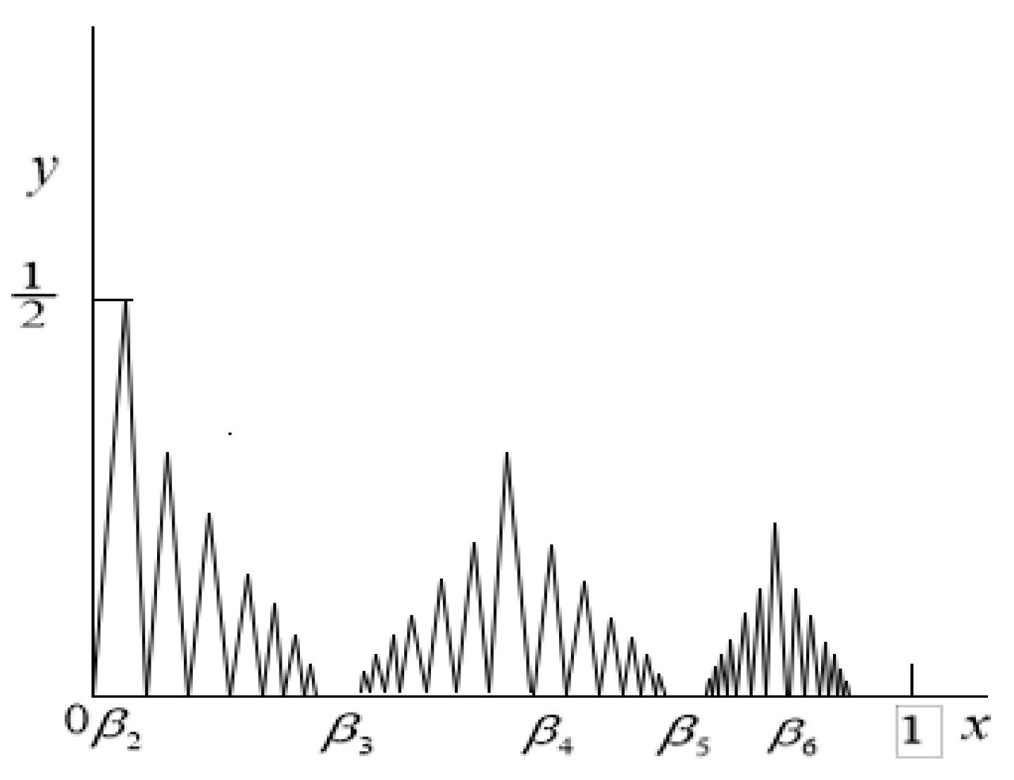
4.5. UVF Contained Infinite UV Points

Theorem 7.

Let $f\left(x\right)$ be a continuous function on I. $f\left(x\right)$ has infinite and countable UV points and only one accumulation point, then

$${dim}_{H}G(f,I)=1.$$

Proof of Theorem 7.

Since $f\left(x\right)$ is a continuous function on I,

$$1\le {dim}_{H}G(f,I)\le {\underline{dim}}_{B}G(f,I).$$

(1) $(0,0)$ is an accumulation point: denote the above countable UV points as

$$x_1>x_2>x_3>\cdots >x_n>\cdots .$$

$\forall \delta >0$, ${dim}_{H}G(f,[0,\delta ])=1$, there is not an accumulation point in other positions, Thus, there exists $E_i\subset I$ and $E_i$ only contains one UV point $x_i$, $E_i\bigcap E_j=\varnothing$ when $i\ne j$. $f\left(x\right)$ only has an UV point on $E_i$ and

$${dim}_{H}G(f,E_i)=1.$$

Denote $E={\displaystyle \bigcup _{i=1}^{\infty }}{E}_i$. By the countable stability of the Hausdorff dimension,

$$\begin{array}{cc}\hfill {dim}_{H}G(f,I)& ={dim}_H(G(f,E)\bigcup G(f,[0,\delta ]))\hfill \\ \hfill & =sup\{{dim}_{H}G(f,E),{dim}_{H}G(f,[0,\delta ])\}=1.\hfill \end{array}$$

Thus,

$${dim}_{H}G(f,I)=1.$$

(2) $(1,0)$ is an accumulation point: denote the above countable UV points as

$$x_1<x_2<x_3<\cdots <x_n<\cdots .$$

$\forall \delta >0$, ${dim}_{H}G(f,[1-\delta ,1])=1$, there is not an accumulation point in other points. There exists $E_i\subset I$ and $E_i$ only contains one UV point $x_i$, $E_i\bigcap E_j=\varnothing$ when $i\ne j$. $f\left(x\right)$ only has an UV point on $E_i$ and

$${dim}_{H}G(f,E_i)=1.$$

Denote $E={\displaystyle \bigcup _{i=1}^{\infty }}{E}_i$.

$$\begin{array}{cc}\hfill {dim}_{H}G(f,I)& ={dim}_H(G(f,E)\bigcup G(f,[0,\delta ]))\hfill \\ \hfill & =sup\{{dim}_{H}G(f,E),{dim}_{H}G(f,[0,\delta ])\}=1.\hfill \end{array}$$

Thus

$${dim}_{H}G(f,I)=1.$$

(3) $x_n\in (0,1),(x_n,0)$ is an accumulation point: $\forall \delta >0$, ${dim}_{H}G(f,[x_n-\delta ,x_n+\delta ])=1$. By the above discussions,

$${dim}_{H}G(f,I)=1.$$

□

Theorem 8.

Let $f\left(x\right)$ be a continuous function containing countable UV points and $f\left(x\right)$ only have an accumulation point on I. If $f\left(x\right)$ is self-similar, then

$${dim}_{H}G(f,I)={dim}_{B}G(f,I)=1.$$

Proof. 

Since $f\left(x\right)$ is a continuous function on I,

$$1\le {dim}_{H}G(f,I)\le {\underline{dim}}_{B}G(f,I).$$

Denote the above uncountable UV points as $x_1,x_2,x_3,\cdots$. There exists $[a_i,x_i]$ and $[a_i,x_i]\bigcap [a_j,x_j]=\varnothing$ when $i\ne j$. Thus, $f\left(x\right)$ only have an UV point on $[a_i,x_i]$ and

$${dim}_{B}G(f,[a_i,x_i])=1.$$

Thus,

$${\overline{dim}}_{MB}G(f,E)=inf\{\underset{i}{sup}{\overline{dim}}_{B}G(f,[a_i,x_i]):E=\bigcup _{i=1}^{N-1}[a_i,x_i]\}=1.$$

Denote $E={\displaystyle \bigcup _{i=1}^{N-1}}[a_i,x_i]$, $F=[a_N,1]$ and $H=\bigcup _{i=1}^{N-1}[x_i,a_{i+1}]$ where $a_1=0$. Further inferences show that $f\left(x\right)$ is a BVF on H and

$${dim}_{H}G(f,H)={dim}_{B}G(f,H)=1.$$

It can be seen from the similar calculation process that

$$\begin{array}{cc}\hfill {\overline{dim}}_{MB}G(f,I)& ={\overline{dim}}_{MB}(G(f,E)\bigcup G(f,F)\bigcup G(f,H))\hfill \\ \hfill & =inf\{sup\{{dim}_{H}G(f,E),{dim}_{H}G(f,F),{dim}_{H}G(f,H)\}\}=1.\hfill \end{array}$$

Since $f\left(x\right)$ is self-similar on I, $G(f,I)$ is compact and

$${\overline{dim}}_B(G(f,I)\bigcap V)={\overline{dim}}_{B}G(f,I)$$

for all open sets V that intersect $G(f,I)$. Thus,

$${\overline{dim}}_{B}G(f,I)={\overline{dim}}_{MB}G(f,I).$$

Notice that the conclusion ${\underline{dim}}_{B}G(f,I)\ge 1$ remains true.

$${dim}_{H}G(f,I)={dim}_{P}G(f,I)={dim}_{MB}G(f,I)={dim}_{B}G(f,I)=1.$$

□

5. Possible Applications in Reinforcement Learning

Since AlphaGo has shown amazing abilities in Go [43,44], reinforcement learning in machine learning has gradually been paid attention and researched by many scholars [45,46,47,48]. The core idea of reinforcement learning is to use the continuous interaction between the agent and the environment to maximize the long-term cumulative return expectation. The agent learns the optimal strategy through the mechanism of trial and error. Taking the expectation of maximizing returns as the goal makes reinforcement learning “foresight”, not just focusing on the immediate situation, so the strategies obtained through reinforcement learning are scientific. Since the optimal strategy can be learned by reinforcement learning, Reinforcement learning has become an emerging method of researching decision theory. At the same time, the learning process of the agent in reinforcement learning is dynamic, and the required data is also generated through interaction with the environment, so a large amount of original label data is not required.

With the advent of deep neural networks, deep reinforcement learning can solve many complex problems. The seemingly complex fractal sets also have special regularity (self-similarity). Therefore, can fractals and fractal dimension be used in the learning process of the agent to speed up the learning speed of the agent or improve the search efficiency of algorithms? This section will introduce several possible applications of fractal and fractal dimension in reinforcement learning.

5.1. The Evaluation Model Based on Fractal Dimension

The main basis of the fractal evaluation model is the fractal dimension. Fractal dimension is an important indicator of system stability. The multi-dimensional vector can be formed by utilizing the parameters, such as actions and states of agents. Many multi-dimensional vectors may establish a special set. The fractal dimension of the set can determine the distance between the current state and the equilibrated state. The equilibrium state is that all agents are in a stable state and there is no motivation to change the current strategy. The main operational flows of the fractal evaluation model are as follows.

Step one: data standardization. The number of states and agents are K, N respectively. State $\mathbb{S}=(s_1,s_2,\cdots ,s_N,a_1,a_2,\cdots ,a_N,r_1,r_2,\cdots ,r_N)$. Standardization is to eliminate the differences caused by the species of each data. Standardized data is $\mathbb{S}=\left(y_{ij}\right)$, $i=1,2,\cdots ,K\in {\mathbb{Z}}^{+}$, $y=1,2,\cdots ,3N\in {\mathbb{Z}}^{+}$.

Step two: weight. $w_j=d_j/{\sum }_{i=1}^N{d}_j$,

where $d_j={max}_{1\le i,k\le K}\mid y_{ij}-y_{kj}\mid$, $j=1,2,\cdots ,N\in {\mathbb{Z}}^{+}$.

Step three: calculate $N\left(r\right)$. The distance used in the algorithm is unified as Euclidean distance. $3N$ data of each state can be regarded as points on each coordinate axis in the 3n-dimensional space. These points constitute a subset of the $3n$-dimensional Euclidean space $E^{3N}$. The distance from each point to the origin is $d_{ij}$ and let $R=max\left(d_{ij}\right)$, $i=1,2,\cdots ,K\in {\mathbb{Z}}^{+}$, $j=1,2,\cdots ,3N\in {\mathbb{Z}}^{+}$. For a specific state, $N\left(r\right)$ is the number of all points satisfying $d_{ij}<r$ and r is the radius of the hypersphere. Keep adjusting the value of radius r until $r=R$ and $N\left(r\right)=N$. When the radius is r, the number of points contained in the hypersphere is $N\left(r\right)={\displaystyle \sum _{i=0}^{3N}}sgn(r-d_{ij})$ and $sgn\left(x\right)$ is a symbolic function,

$$sgn\left(x\right)=\left\{\begin{array}{cc}1,\hfill & x>0\hfill \\ 0,\hfill & x\le 0\hfill \end{array}\right.$$

Step four: calculate the fractal dimension. $D=logN\left(r\right)/logr$.

From the above calculation process, the number of sample points contained in the hypersphere with r will change continuously as the radius alters. At the same time, the graph of the function formed by the above standardized data points is usually non-linear. The fractal dimension D in this step can be fitted by the least square method,

$$D=\frac{3N{\displaystyle \sum _{i=1}^{3N}}logN\left(r_i\right)log{r}_i-{\displaystyle \sum _{i=1}^{3N}}logN\left(r_i\right){\displaystyle \sum _{i=1}^{3N}}log{r}_i}{3N{\displaystyle \sum _{i=1}^{3N}}{\left(log{r}_i\right)}^2-{\left({\displaystyle \sum _{i=1}^{3N}}log{r}_i\right)}^2}.$$

At present, most reinforcement learning algorithms are based on global information. However, due to the limitations of communication and observation, the agent cannot obtain all the information in practical. Therefore, the MDP(Markov decision process) model used to solve basic reinforcement learning problems is not applicable. Researchers establish the POMDP(Partially observable markov decision process) model [49,50] to solve partially observable reinforcement learning problems. The main solutions include function approximation, opponent modeling, and graph theory.

Fractal dimension is another new idea to optimize POMDP. The theoretical foundation of using fractal dimension to evaluate stability is mainly based on the Lyapunov stability theory. The larger fractal dimension of the set, the more stable points in the set. Therefore, the set with lager fractal dimension is more stable than the set with small fractal dimension under the same disturbance. The advantage of this method is that the agent does not need to know global information. The strategy selection of agents can be guided by the fractal dimension, and the correct strategy direction can optimize the algorithm. At the same time, for a game where there is no pure strategy Nash equilibrium, it is still possible to compare the distance between any two situations and the equilibrium state by calculating the fractal dimension.

5.2. The Convergence Model Based on Fractal Attractor

At present, the convergence of most reinforcement learning algorithms lacks rigorous proofs. However, due to the powerful fitting ability of multiple neural networks [51,52,53], the algorithm can converge better in various experimental environments. The convergence obtained in the experiment cannot effectively understand the essence of the problem and optimize the existing algorithm. Obviously, the convergence of an algorithm is the fixed point of a particular function mathematically. Solving the fixed point problem can also be transformed into an attractor in fractal theory. Therefore, the convergence of the algorithm can be verified by calculating the existence of attractors. Surprisingly, the calculation of attractors has theoretical guarantees. Therefore, can the Bellman equation in reinforcement learning be regarded as an iterative function system, and then its solution is the attractor of the iterative function system? The idea of the model is shown in Figure 9.

The advantage of this convergence model lies in its versatility, which can prove the convergence of a class of similar algorithms. The method of theoretical proof is conducive to finding the essence of the problem, so as to provide different ideas for the optimization algorithm.

5.3. The Random Search Algorithm Based on Fractal

Exploration and utilization is one of the important research directions in deep reinforcement learning. The goal of exploration is to find more information about the environment, and the purpose of utilization is to use the known environmental information to maximize rewards. In short, exploration is to try behaviors that have not yet been tried, while utilization is to choose the next action from the knowledge that agents have already mastered. The balance between exploration and utilization is the basic issue of reinforcement learning. In deep reinforcement learning tasks, in order to obtain the best strategy, it is often necessary to collect more information. For solving the problem of exploration and utilization, researchers have proposed many classic methods. The $ϵ$-greedy method is a commonly used strategy for greedy exploration.

However, the exploratory efficiency of this method is not good. Fractals generally have the following characteristics. One is that both the whole and the part have irregularities, and the other is that the internal structure has self-similarity and unevenness. The search method based on the fractal structure can reduce the search time as much as possible on the basis of ensuring that all spaces are explored. Due to the self-similar structure of the fractal, the algorithm does not always need to repeat the previous training during the training process. Thus the way can reduce a lot of unnecessary training time. Therefore, whether the above-mentioned characteristics of fractal can be used to achieve efficient search is looking forward to follow-up research and discussion. At present, there has been a lot of research on using fractals to improve search efficiency [54,55,56], but these algorithms can still continue to be optimized.

6. Conclusions

This manuscript systematically sorts out the conclusions about one-dimensional continuous functions. The Box dimension of bounded variation functions and the functions with the Weyl fractional integral are both one. The Box dimension of continuous functions that satisfy the Lipschitz condition is also one. These results also fully show that fractional calculus does not increase the dimensionality of functions. This conclusion seems simple, but no one seems to have carried out a rigorous proof. The structure of unbounded variation function is more complicated. The construction process of several special unbounded variation functions is displayed firstly, and a lot of general conclusions about unbounded variation functions are proved by using UV points. Combined with the self-similarity, the conclusions of the fractal dimension of some special functions are also strictly proved. These conclusions are very helpful for perfecting the theory of unbounded variation. At the same time, in order to increase the practical significance of the above conclusions, some applications of fractal and fractal dimension in reinforcement learning are also introduced. On the one hand, these works can sort out the current results, and on the other hand, some useful ideas and research directions can also be shown to other researchers. The evaluation model based on fractal dimension proposed in this manuscript can effectively accelerate the convergence speed of many reinforcement learning algorithms by using fractal dimension to judge the stability of any state. This model is an important result of the combination of the two theories, and it is believed that more fractal theories will be applied to reinforcement learning.

However, the research on one-dimensional continuous functions is far from over. In particular, what are the necessary and sufficient conditions for the conversion between unbounded variation and bounded variation? Are there other theories and tools that can be used to study one-dimensional continuous functions? Can existing relevant conclusions about one-dimensional continuous functions be extended to multi-dimensional continuous functions? Can the conclusion of the unbounded variation function be used in other fields?

References

- Srivastava, H.M.; Kashuri, A.; Mohammed, P.O.; Nonlaopon, K. Certain inequalities pertaining to some new generalized fractional integral operators. Fractal Fract. 2021, 5, 160. [Google Scholar] [CrossRef]
- Khan, M.B.; Noor, M.A.; Abdeljawad, T.; Mousa, A.A.A.; Abdalla, B.; Alghamdi, S.M. LR-preinvex interval-valued functions and Riemann–Liouville fractional integral inequalities. Fractal Fract. 2021, 5, 243. [Google Scholar] [CrossRef]
- Machado, J.T.; Mainardi, F.; Kiryakova, V. Fractional calculus: Quo vadimus? (Where are we going?). Fract. Calc. Appl. Anal. 2015, 18, 495–526. [Google Scholar] [CrossRef]
- Butera, S.; Paola, M.D. A physically based connection between fractional calculus and fractal geometry. Ann. Phys. 2014, 350, 146–158. [Google Scholar] [CrossRef]
- Kolwankar, K.M.; Gangal, A.D. Fractional differentiability of nowhere differentiable functions and dimensions. Chaos Solitons Fractals 1996, 6, 505–513. [Google Scholar] [CrossRef] [Green Version]
- Kolwankar, K.M.; Gangal, A.D. Hölder exponent of irregular signals and local fractional derivatives. Pramana J. Phys. 1997, 48, 49–68. [Google Scholar] [CrossRef] [Green Version]
- Nigmatullin, R.R.; Baleanu, D. Relationships between 1D and space fractals and fractional integrals and their applications in physics. In Applications in Physics, Part A; De Gruyter: Berlin, Germany, 2019; Volume 4, pp. 183–220. [Google Scholar]
- Tatom, F.B. The relationship between fractional calculus and fractals. Fractals 1995, 3, 217–229. [Google Scholar] [CrossRef]
- Zähle, M.; Ziezold, H. Fractional derivatives of weierstrass-type functions. J. Comput. Appl. Math. 1996, 76, 265–275. [Google Scholar] [CrossRef] [Green Version]
- Liang, Y.S. The relationship between the Box dimension of the Besicovitch functions and the orders of their fractional calculus. Appl. Math. Comput. 2008, 200, 197–207. [Google Scholar] [CrossRef]
- Ruan, H.J.; Su, W.Y.; Yao, K. Box dimension and fractional integral of linear fractal interpolation functions. J. Approx. Theory 2009, 161, 187–197. [Google Scholar] [CrossRef] [Green Version]
- Liang, Y.S. Box dimensions of Riemann-Liouville fractional integrals of continuous functions of bounded variation. Nonlinear Anal. 2010, 72, 4304–4306. [Google Scholar] [CrossRef]
- Liang, Y.S. Fractal dimension of Riemann-Liouville fractional integral of 1-dimensional continuous functions. Fract. Calc. Appl. Anal. 2018, 21, 1651–1658. [Google Scholar] [CrossRef]
- Wu, J.R. On a linearity between fractal dimensions and order of fractional calculus in Hölder space. Appl. Math. Comput. 2020, 385, 125433. [Google Scholar] [CrossRef]
- Verma, S.; Viswanathan, P. A note on Katugampola fractional calculus and fractal dimensions. Appl. Math. Comput. 2018, 339, 220–230. [Google Scholar] [CrossRef]
- Verma, S.; Viswanathan, P. Bivariate functions of bounded variation: Fractal dimension and fractional integral. Indag. Math. 2020, 31, 294–309. [Google Scholar] [CrossRef] [Green Version]
- Bush, K.A. Continuous functions without derivatives. Am. Math. Mon. 1952, 59, 222–225. [Google Scholar] [CrossRef]
- Shen, W.X. Hausdorff dimension of the graphs of the classical Weierstrass functions. Math. Z. 2018, 289, 223–266. [Google Scholar] [CrossRef] [Green Version]
- Su, W.Y. Construction of fractal calculus. Sci. China Math. Chin. Ser. 2015, 45, 1587–1598. [Google Scholar] [CrossRef]
- Xie, T.F.; Zhou, S.P. On a class of fractal functions with graph box dimension 2. Chaos Solitons Fractals 2004, 22, 135–139. [Google Scholar] [CrossRef]
- Liang, Y.S.; Su, W.Y. Von Koch curves and their fractional calculus. Acta Math. Sin. Chin. Ser. 2011, 54, 227–240. [Google Scholar]
- Wang, J.; Yao, K. Construction and analysis of a special one-dimensional continuous functions. Fractals 2017, 25, 1750020. [Google Scholar] [CrossRef]
- Wang, J.; Yao, K.; Liang, Y.S. On the connection between the order of Riemann-Liouvile fractional falculus and Hausdorff dimension of a fractal function. Anal. Theory Appl. 2016, 32, 283–290. [Google Scholar] [CrossRef]
- Falconer, K.J. Fractal Geometry: Mathematical Foundations and Applications; John Wiley Sons Inc.: Chicheste, PA, USA, 1990. [Google Scholar]
- Wen, Z.Y. Mathematical Foundations of Fractal Geometry; Science Technology Education Publication House: Shanghai, China, 2000. (In Chinese) [Google Scholar]
- Hu, T.Y.; Lau, K.S. Fractal dimensions and singularities of the weierstrass type functions. Trans. Am. Math. Soc. 1993, 335, 649–665. [Google Scholar] [CrossRef]
- Zheng, W.X.; Wang, S.W. Real Function and Functional Analysis; High Education Publication House: Beijing, China, 1980. (In Chinese) [Google Scholar]
- Tian, L. The estimates of Hölder index and the Box dimension for the Hadamard fractional integral. Fractals 2021, 29, 2150072. [Google Scholar] [CrossRef]
- Wang, C.Y. R-L Algorithm: An approximation algorithm for fractal signals based on fractional calculus. Fractals 2020, 24, 2150243. [Google Scholar] [CrossRef]
- Oldham, K.B.; Spanier, J. The Fractional Calculus; Academic Press: New York, NY, USA, 1974. [Google Scholar]
- Teodoro, G.S.; Machado, J.A.; Oliveira, E.C. A review of definitions of fractional derivatives and other operators. J. Comput. Phys. 2019, 388, 195–208. [Google Scholar] [CrossRef]
- Kiryakova, V.S. Generalized Fractional Calculus and Applications; CRC Press: Boca Raton, FL, USA, 1993. [Google Scholar]
- Miller, K.S.; Ross, B. An Introduction to the Fractional Calculus and Fractional Differential Equations; John Wiley Sons Inc.: New York, NY, USA, 1976. [Google Scholar]
- Podlubny, I. Geometric and physical interpretation of fractional integration and fractional differentiation. Fract. Calc. Appl. Anal. 2002, 5, 367–386. [Google Scholar]
- Mu, L.; Yao, K.; Wang, J. Box dimension of weyl fractional integral of continuous functions with bounded variation. Anal. Theory Appl. 2016, 32, 174–180. [Google Scholar] [CrossRef]
- Kilbas, A.A.; Titioura, A.A. Nonlinear differential equations with marchaud-hadamard-type fractional derivative in the weighted sapce of summable functions. Math. Model. Anal. 2007, 12, 343–356. [Google Scholar] [CrossRef]
- Tian, L. Hölder continuity and box dimension for the Weyl fractional integral. Fractals 2020, 28, 2050032. [Google Scholar] [CrossRef]
- Yao, K.; Liang, Y.S.; Su, W.Y.; Yao, Z.Q. Fractal dimension of fractional derivative of self-affine functions. Acta Math. Sin. Chin. Ser. 2013, 56, 693–698. [Google Scholar]
- Xu, Q. Fractional integrals and derivatives to a class of functions. J. Xuzhou Norm. Univ. 2006, 24, 19–23. [Google Scholar]
- Stein, E.M. Singular Integrals and Differentiability Properties of Functions; Princeton University Press: Princeton, NJ, USA, 1970. [Google Scholar]
- Liang, Y.S.; Su, W.Y. Fractal dimensions of fractional integral of continuous functions. Acta Math. Sin. 2016, 32, 1494–1508. [Google Scholar] [CrossRef]
- Liang, Y.S.; Zhang, Q. 1-dimensional continuous functions with uncountable unbounded variation points. Chin. J. Comtemporary Math. 2018, 39, 129–136. [Google Scholar]
- Silver, D.; Schrittwieser, J.; Simonyan, K.; Antonoglou, I.; Huang, A.; Guez, A.; Hubert, T.; Baker, L.; Lai, M.; Bolton, A.; et al. Mastering the game of go without human knowledge. Nature 2017, 550, 354–359. [Google Scholar] [CrossRef]
- Magnani, L. AlphaGo, Locked Strategies, and Eco-Cognitive Openness; Eco-Cognitive Computationalism Springer: Cham, Switzerland, 2021; pp. 45–71. [Google Scholar]
- Liu, S.; Pan, Z.; Cheng, X. A novel fast fractal image compression method based on distance clustering in high dimensional sphere surface. Fractals 2017, 25, 1740004. [Google Scholar] [CrossRef] [Green Version]
- Li, S.; Wu, Y.; Cui, X.; Dong, H.; Fang, F.; Russell, S. Robust multi-agent reinforcement learning via minimax deep deterministic policy gradient. Proc. Aaai Conf. Artif. Intell. 2019, 33, 4213–4220. [Google Scholar] [CrossRef] [Green Version]
- Li, G.; Jiang, B.; Zhu, H.; Che, Z.; Liu, Y. Generative attention networks for multi-agent behavioral modeling. Proc. Aaai Conf. Artif. Intell. 2020, 34, 7195–7202. [Google Scholar] [CrossRef]
- Liu, S.; Wang, S.; Liu, X.Y.; Gandomi, A.H.; Daneshmand, M.; Muhammad, K.; de Albuquerque, V.H.C. Human Memory Update Strategy: A multi-layer template update mechanism for remote visual monitoring. IEEE Trans. Multimed. 2021, 23, 2188–2198. [Google Scholar] [CrossRef]
- Hoerger, M.; Kurniawati, H. An on-line POMDP solver for continuous observation spaces. In Proceedings of the 2021 IEEE International Conference on Robotics and Automation (ICRA), Xi’an, China, 30 May–5 June 2021; pp. 7643–7649. [Google Scholar]
- Igl, M.; Zintgraf, L.; Le, T.A.; Wood, F.; Whiteson, S. Deep variational reinforcement learning for POMDPs. Int. Conf. Mach. Learn. 2018, 16, 2117–2126. [Google Scholar]
- Zhou, Z.H. Neural Networks. In Machine Learning; Springer: Singapore, 2021. [Google Scholar]
- Yang, L.; Zhang, R.Y.; Li, L.; Xie, X. Simam: A simple parameter-free attention module for convolutional neural networks. Int. Conf. Mach. Learn. 2021, 26, 11863–11874. [Google Scholar]
- Almatroud, A.O. Extreme multistability of a fractional-order discrete-time neural network. Fractal Fract. 2021, 5, 202. [Google Scholar] [CrossRef]
- Alomoush, M.I. Optimal combined heat and power economic dispatch using stochastic fractal search algorithm. J. Mod. Power Syst. Clean Energy 2020, 8, 276–286. [Google Scholar] [CrossRef]
- Tran, T.T.; Truong, K.H. Stochastic fractal search algorithm for reconfiguration of distribution networks with distributed generations. Ain Shams Eng. J. 2020, 11, 389–407. [Google Scholar] [CrossRef]
- Pham, L.H.; Duong, M.Q.; Phan, V.D.; Nguyen, T.T.; Nguyen, H.N. A high-performance stochastic fractal search algorithm for optimal generation dispatch problem. Energies 2019, 12, 1796. [Google Scholar] [CrossRef] [Green Version]
Publisher’s Note: MDPI stays neutral with regard to jurisdictional claims in published maps and institutional affiliations. |
© 2022 by the authors. Licensee MDPI, Basel, Switzerland. This article is an open access article distributed under the terms and conditions of the Creative Commons Attribution (CC BY) license (https://creativecommons.org/licenses/by/4.0/).
Share and Cite
Jun, W.; Lei, C.; Bin, W.; Hongtao, G.; Wei, T. Overview of One-Dimensional Continuous Functions with Fractional Integral and Applications in Reinforcement Learning. Fractal Fract. 2022, 6, 69. https://doi.org/10.3390/fractalfract6020069
Jun W, Lei C, Bin W, Hongtao G, Wei T. Overview of One-Dimensional Continuous Functions with Fractional Integral and Applications in Reinforcement Learning. Fractal and Fractional. 2022; 6(2):69. https://doi.org/10.3390/fractalfract6020069
Chicago/Turabian StyleJun, Wang, Cao Lei, Wang Bin, Gong Hongtao, and Tang Wei. 2022. "Overview of One-Dimensional Continuous Functions with Fractional Integral and Applications in Reinforcement Learning" Fractal and Fractional 6, no. 2: 69. https://doi.org/10.3390/fractalfract6020069