
A General Return-Mapping Framework for Fractional Visco-Elasto-Plasticity

Abstract
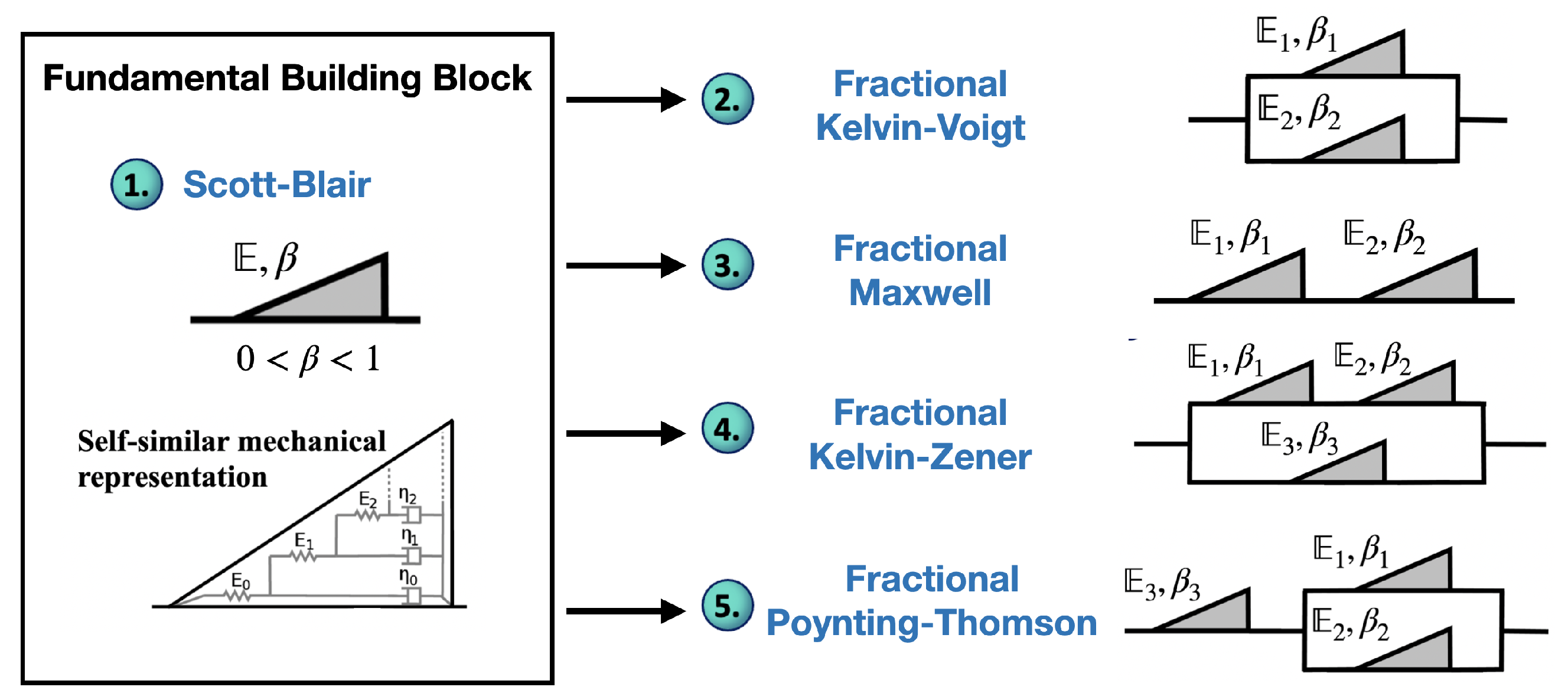
:1. Introduction
- We perform a full discretization of fractional viscoelastic models prior to the definition of trial states, which allows a linear decomposition between final and trial stresses regardless of the employed models.
- The fractional return-mapping algorithm is fully implicit for linear viscoelastic rheology and semi-implicit for quasi-linear viscoelasticity.
- Due to the full-discretization before the return-mapping procedure, the operations involving the plastic-slip are memoryless, which resembles return-mapping steps from the classical elasto-plasticity.
- The correction (return-mapping) step has the same structure regardless of the employed viscoelastic models.
2. Definitions of Fractional Calculus
3. Fractional Viscoelasticity
3.1. Linear Viscoelasticity
3.2. Quasi-Linear Fractional Viscoelasticity
4. Fractional Visco-Elasto-Plasticity
5. A Class of Return-Mapping Algorithms for Fractional Visco-Elasto-Plasticity
5.1. Time-Fractional Integration of Viscoelastic Models
5.2. Time-Fractional Integration of Visco-Plasticity
5.3. Generalized Fractional Return-Mapping Algorithm (Algorithm 1)
| Algorithm 1: Fractional return-mapping algorithm. |
|
Comparison of the Return-Mapping Algorithm to the Existing Approaches
6. Numerical Tests
7. Conclusions
- The trial states were taken after full discretization of stress and internal variables, which allowed a straightforward decomposition of the yield function into the final and trial states.
- The developed return-mapping procedure is fully implicit for linear viscoelastic models and semi-implicit for quasi-linear viscoelasticity. For simplicity, the chosen numerical discretization for fractional derivatives was an L1 finite-difference approach.
- Our correction step for visco-plasticity had the same structure for all viscoelastic models with the only difference being a scaling discretization constant.
- We carried out numerical experiments with analytical and reference solutions that demonstrated the global accuracy, surprisingly even in some instances with general loading/unloading conditions.
- The developed return-mapping discretization was compared to an existing approach, and the difference between discretizations relied on cases with extensive plastic history and high strain rates.
Author Contributions
Funding
Institutional Review Board Statement
Informed Consent Statement
Data Availability Statement
Conflicts of Interest
Appendix A. Proof of Proposition 1
Appendix B. Discretization Constants and Terms for Fractional Viscoelastic Models
Appendix C. Return-Mapping Derivation for the Fractional Kelvin–Zener Model
References
- Okajima, T. Nanorheology of Living Cells. In The World of Nano-Biomechanics; Ikai, A., Ed.; Elsevier: Amsterdam, The Netherlands, 2017; pp. 249–265. [Google Scholar]
- De Sousa, J.; Freire, R.; Sousa, F.; Radmacher, M.; Silva, A.; Ramos, M.; Monteiro-Moreira, A.; Mesquita, F.; Moraes, M.; Montenegro, R.; et al. Double power-law viscoelastic relaxation of living cells encodes motility trends. Sci. Rep. 2020, 10, 4749. [Google Scholar] [CrossRef] [Green Version]
- Naghibolhosseini, M.; Long, G.R. Fractional-order modelling and simulation of human ear. Int. J. Comput. Math. 2018, 95, 1257–1273. [Google Scholar] [CrossRef]
- Guo, J.; Yin, Y.; Peng, G. Fractional-order viscoelastic model of musculoskeletal tissues: Correlation with fractals. Proc. R. Soc. A 2021, 477, 20200990. [Google Scholar] [CrossRef]
- Suzuki, J.L.; Tuttle, T.G.; Roccabianca, S.; Zayernouri, M. A data-driven memory-dependent modeling framework for anomalous rheology: Application to urinary bladder tissue. Fractal Fract. 2021, 5, 223. [Google Scholar] [CrossRef]
- Martin, P.; Hudspeth, A. Compressive nonlinearity in the hair bundle’s active response to mechanical stimulation. Proc. Natl. Acad. Sci. USA 2001, 98, 14386–14391. [Google Scholar] [CrossRef] [Green Version]
- Choi, J.S.; Kim, N.J.; Klemuk, S.; Jang, Y.H.; Park, I.S.; Ahn, K.H.; Lim, J.Y.; Kim, Y.M. Preservation of viscoelastic properties of rabbit vocal folds after implantation of hyaluronic acid-based biomaterials. Otolaryngol. Head Neck Surg. 2012, 147, 515–521. [Google Scholar] [CrossRef]
- Stamenović, D.; Rosenblatt, N.; Montoya-Zavala, M.; Matthews, B.; Hu, S.; Suki, B.; Wang, N.; Ingber, D. Rheological Behavior of Living Cells Is Timescale-Dependent. Biophys. J. 2007, 93, L39–L41. [Google Scholar] [CrossRef] [Green Version]
- Vincent, J. Structural Biomaterials; Princeton University Press: Princeton, NJ, USA, 2012. [Google Scholar]
- Kapnistos, M.; Lang, M.; Vlassopoulos, D.; Pyckhout-Hintzen, D.; Richter, D.; Cho, D.; Chang, T.; Rubinstein, M. Unexpected power-law stress relaxation of entangled ring polymers. Nat. Mater. 2008, 7, 997–1002. [Google Scholar] [CrossRef]
- Pajerowski, J.; Dahl, K.; Zhong, F.; Sammak, P.; Discher, D. Physical plasticity of the nucleus in stem cell differentiation. Proc. Natl. Acad. Sci. USA 2007, 40, 15619–15624. [Google Scholar] [CrossRef]
- Bonadkar, N.; Gerum, R.; Kuhn, M.; Sporer, M.; Lippert, A.; Schneider, W.; Aifantis, K.; Fabry, B. Mechanical plasticity of cells. Nat. Mater. 2016, 15, 1090–1094. [Google Scholar]
- Suzuki, J.L.; Gulian, M.; Zayernouri, M.; D’Elia, M. Fractional modeling in action: A survey of nonlocal models for subsurface transport, turbulent flows, and anomalous materials. J. Peridynamics Nonlocal Model. 2022, 1–68. [Google Scholar] [CrossRef]
- Suzuki, J.; Zayernouri, M.; Bittencourt, M.; Karniadakis, G. Fractional-order uniaxial visco-elasto-plastic models for structural analysis. Comput. Methods Appl. Mech. Eng. 2016, 308, 443–467. [Google Scholar] [CrossRef] [Green Version]
- Xiao, R.; Sun, H.; Chen, W. A finite deformation fractional viscoplastic model for the glass transition behavior of amorphous polymers. Int. J. Nonlinear Mech. 2017, 93, 7–14. [Google Scholar] [CrossRef]
- Suzuki, J.; Zhou, Y.; D’Elia, M.; Zayernouri, M. A thermodynamically consistent fractional visco-elasto-plastic model with memory-dependent damage for anomalous materials. Comput. Methods Appl. Mech. Eng. 2021, 373, 113494. [Google Scholar] [CrossRef]
- Sumelka, W. Application of fractional continuum mechanics to rate independent plasticity. Acta Mech. 2014, 225, 3247–3264. [Google Scholar] [CrossRef] [Green Version]
- Sumelka, W. Fractional Viscoplasticity. Mech. Res. Commun. 2014, 56, 31–36. [Google Scholar] [CrossRef]
- Sun, Y.; Sumelka, W. Fractional viscoplastic model for soils under compression. Acta Mech. 2019, 230, 3365–3377. [Google Scholar] [CrossRef]
- Sun, H.; Zhang, Y.; Baleanu, D.; Chen, W.; Chen, Y. A new collection of real world applications of fractional calculus in science and engineering. Commun. Nonlinear Sci. Numer. Simul. 2018, 64, 213–231. [Google Scholar] [CrossRef]
- Podlubny, I. Fractional Differential Equations: An Introduction to Fractional Derivatives, Fractional Differential Equations, to Methods of Their Solution and Some of Their Applications; Elsevier: Amsterdam, The Netherlands, 1998. [Google Scholar]
- Mainardi, F.; Spada, G. Creep, Relaxation and Viscosity Properties for Basic Fractional Models in Rheology. arXiv 2011, arXiv:1110.3400v1. [Google Scholar] [CrossRef] [Green Version]
- Blair, G.; Veinoglou, B.; Caffyn, B. Limitations of the Newtonian time scale in relation to non-equilibrium rheological states and a theory of quasi-properties. Proc. R. Soc. A Math. Phys. Eng. Sci. 1947, 189, 69–87. [Google Scholar]
- Jaishankar, A.; McKinley, G. Power-law rheology in the bulk and at the interface: Quasi-properties and fractional constitutive equations. Proc. R. Soc. A 2013, 469, 20120284. [Google Scholar] [CrossRef] [Green Version]
- Schiessel, H.; Blumen, A. Hierarchical analogues to fractional relaxation equations. J. Phys. A Math. Gen. 1993, 26, 5057–5069. [Google Scholar] [CrossRef]
- McKinley, G.; Jaishankar, A. Critical Gels, Scott Blair and the Fractional Calculus of Soft Squishy Materials. In Proceedings of the Bingham Lecture, 85th Annual Meeting of the Society of Rheology, Montréal, QC, Canada, 13–17 October 2013. [Google Scholar]
- Lion, A. On the thermodynamics of fractional damping elements. Contin. Mech. Thermodyn. 1997, 9, 83–96. [Google Scholar] [CrossRef]
- Bonfanti, A.; Kaplan, J.L.; Charras, G.; Kabla, A.J. Fractional viscoelastic models for power-law materials. Soft Matter 2020, 16, 6002–6020. [Google Scholar] [CrossRef]
- Schiessel, H. Generalized viscoelastic models: Their fractional equations with solutions. J. Phys. A Math. Gen. 1995, 28, 6567–6584. [Google Scholar] [CrossRef]
- Fung, Y.C. Biomechanics: Mechanical Properties of Living Tissues; Springer Science & Business Media: Berlin/Heidelberg, Germany, 2013. [Google Scholar]
- Craiem, D.; Rojo, F.; Atienza, J.; Armentano, R.; Guinea, G. Fractional-order viscoelasticity applied to describe uniaxial stress relaxation of human arteries. Phys. Med. Biol 2008, 53, 4543. [Google Scholar] [CrossRef] [Green Version]
- Simo, J.; Hughes, T. Computational Inelasticity; Springer: Berlin/Heidelberg, Germany, 1998. [Google Scholar]
- Lin, Y.; Xu, C. Finite difference/spectral approximations for the time-fractional diffusion equation. J. Comput. Phys. 2007, 225, 1533–1552. [Google Scholar] [CrossRef]
- Zeng, F.; Turner, I.; Burrage, K. A stable fast time-stepping method for fractional integral and derivative operators. J. Sci. Comput. 2018, 77, 283–307. [Google Scholar] [CrossRef] [Green Version]
- Naghibolhosseini, M. Estimation of Outer-Middle Ear Transmission Using DPOAEs and Fractional-Order Modeling of Human Middle Ear; City University of New York: New York, NY, USA, 2015. [Google Scholar]
- Suzuki, J.L.; Kharazmi, E.; Varghaei, P.; Naghibolhosseini, M.; Zayernouri, M. Anomalous nonlinear dynamics behavior of fractional viscoelastic beams. J. Comput. Nonlinear Dyn. 2021, 16, 111005. [Google Scholar] [CrossRef]
- Branco, A.; Todorovic Fabro, A.; Gonçalves, T.M.; Garcia Martins, R.H. Alterations in extracellular matrix composition in the aging larynx. Otolaryngol. Head Neck Surg. 2015, 152, 302–307. [Google Scholar] [CrossRef]
- Ferster, A.P.; Malmgren, L.T. Cellular and Molecular Mechanisms of Aging of the Vocal Fold. In Voice Science; Sataloff, R.T., Ed.; Plural Publishing Inc.: San Diego, CA, USA, 2017; pp. 157–167. [Google Scholar]
- de Moraes, E.A.B.; Suzuki, J.L.; Zayernouri, M. Atomistic-to-meso multi-scale data-driven graph surrogate modeling of dislocation glide. Comput. Mater. Sci. 2021, 197, 110569. [Google Scholar] [CrossRef]
- de Moraes, E.A.B.; D’Elia, M.; Zayernouri, M. Nonlocal Machine Learning of Micro-Structural Defect Evolutions in Crystalline Materials. arXiv 2022, arXiv:2205.05729. [Google Scholar] [CrossRef]


| – | – | – | ||||||
| 1.8197 | 1.4895 | 1.0981 | ||||||
| 1.8294 | 1.4929 | 1.0991 | ||||||
| 1.8374 | 1.4951 | 1.0995 | ||||||
| 1.8440 | 1.4966 | 1.0998 | ||||||
| 1.8497 | 1.4977 | 1.0999 | ||||||
Publisher’s Note: MDPI stays neutral with regard to jurisdictional claims in published maps and institutional affiliations. |
© 2022 by the authors. Licensee MDPI, Basel, Switzerland. This article is an open access article distributed under the terms and conditions of the Creative Commons Attribution (CC BY) license (https://creativecommons.org/licenses/by/4.0/).
Share and Cite
Suzuki, J.L.; Naghibolhosseini, M.; Zayernouri, M. A General Return-Mapping Framework for Fractional Visco-Elasto-Plasticity. Fractal Fract. 2022, 6, 715. https://doi.org/10.3390/fractalfract6120715
Suzuki JL, Naghibolhosseini M, Zayernouri M. A General Return-Mapping Framework for Fractional Visco-Elasto-Plasticity. Fractal and Fractional. 2022; 6(12):715. https://doi.org/10.3390/fractalfract6120715
Chicago/Turabian StyleSuzuki, Jorge L., Maryam Naghibolhosseini, and Mohsen Zayernouri. 2022. "A General Return-Mapping Framework for Fractional Visco-Elasto-Plasticity" Fractal and Fractional 6, no. 12: 715. https://doi.org/10.3390/fractalfract6120715