
Multi-Fractality, Universality and Singularity in Turbulence

SPEC, CEA, CNRS, Université Paris-Saclay, CEA Saclay, 91191 Gif-sur-Yvette, France
Fractal Fract. 2022, 6(10), 613; https://doi.org/10.3390/fractalfract6100613
Submission received: 13 September 2022
/
Revised: 12 October 2022
/
Accepted: 13 October 2022
/
Published: 20 October 2022
(This article belongs to the Special Issue Multifractals, Turbulence and Complexity in Geoscience and Space Science)
Abstract
:In most geophysical flows, vortices (or eddies) of all sizes are observed. In 1941, Kolmogorov devised a theory to describe the hierarchical organization of such vortices via a homogeneous self-similar process. This theory correctly explains the universal power-law energy spectrum observed in all turbulent flows. Finer observations however prove that this picture is too simplistic, owing to intermittency of energy dissipation and high velocity derivatives. In this review, we discuss how such intermittency can be explained and fitted into a new picture of turbulence. We first discuss how the concept of multi-fractality (invented by Parisi and Frisch in 1982) enables to generalize the concept of self-similarity in a non-homogeneous environment and recover a universality in turbulence. We further review the local extension of this theory, and show how it enables to probe the most irregular locations of the velocity field, in the sense foreseen by Lars Onsager in 1949. Finally, we discuss how the multi-fractal theory connects to possible singularities, in the real or in the complex plane, as first investigated by Frisch and Morf in 1981.
1. Introduction
Fluids are an essential component of our environment: our body is made of 65 percent of water, oceans cover two-thirds of the surface of our planet, which is itself surrounded by a fluid atmosphere. Thanks to satellites, we now have a global view of the dynamics and structure of fluids at such geophysical scales. Figure 1a, taken in South Atlantic Ocean by NASA, is a typical example of swirling motions that are observed at the surface of the ocean, or in the atmosphere. These swirling motions trace vortices, a basic feature of any turbulent flow. If you look carefully at the picture, you’ll notice that vortices have a wide range of scales. A first attempt to quantify their organization was made in 1962 [1], by velocity measurements inside the so-called Seymour narrows, a 5 km section of the Discovery Passage in British Columbia known for strong tidal currents. The Fourier energy spectrum of these measurements is shown in Figure 1b: one sees that the spectrum exhibits a well-defined power-law scaling, characteristic of a hierarchical organization of vortices. The exponent of the power-law is −5/3 and was predicted in 1941 by Kolmogorov [2], using a theoretical analysis of the Navier-Stokes equations (NSE), which are supposed to be the relevant model for most geophysical flows. Later, when technological progress enabled the numerical simulations of the NSE, power-law spectra were indeed observed for solutions of the NSE at large enough Reynolds number, as shown in Figure 1b.
Kolmogorov analysis is based on a few symmetry assumptions (homogeneity, stationarity, self-similarity) that highlight the universal character of the energy spectrum, when plotted in non-dimensional variables involving only the viscosity and the energy input . This is well illustrated by Figure 1b, where we see that all energy spectra collapse, provided the spectra are non-dimensionalized by and the wavenumber by , the Kolmogorov length.
This success of Kolmogorov theory fed the hope of that turbulence could be simply modeled by a self-similar process, resulting in a universal hierarchy of vortices when expressed in units of and . If such hopes were true, universality should extend to higher moments of the velocity field u besides the second and third one, already captured by Kolmogorov theory. To check this, one can build the velocity structure functions defined as:
where is a measure of the velocity at scale ℓ and denotes a statistical average. In his theory, Kolmogorov used , the velocity increment over a distance ℓ. The Fourier energy spectrum being the Fourier transform of , we have by Kolmogorov theory: , where is the Kolmogorov velocity. Kolmogorov theory also predicts that .
For practical reasons, we shall sometimes use another definition of , based on wavelet transform. We thus define more generally:
where , and is any function of zero average. An example is the derivative of a Gaussian, , where .
Kolmogorov theory (hereafter K41) predicts that is a constant, independent of ℓ. More generally, Geneste et al. [3] showed that K41 universality can be checked by plotting:
If the K41 universality holds, all curves collapse on universal lines depending only on p. Further, if turbulence is self-similar, the universal functions are all constant, depending only on p. We can use the DNS data of Figure 1b to check K41 universality. This is shown in Figure 2. Obviously, for , the data do not collapse on a constant universal curve, meaning that neither K41 universality nor self-similarity hold for the DNS. We cannot perform the same check on the data taken in the Seymour narrows (they are not available anymore) but we can try the same check on data taken in water [3], in a von Karman laboratory experiment mimicking flow circulation on Earth [4]. The result is shown in Figure 2a. From this, we see that K41 universality does not hold either for the experimental measurements.
Obviously, Kolmogorov theory is incomplete, as it cannot explain behaviour of moments higher than 3. What can be wrong? Besides NSE, Kolmogorov uses three symmetry hypotheses: stationarity, homogeneity and self-similarity. The last hypothesis is obviously broken by the data, because except for , the ratio is never constant for any data. Breaking of the universality, on the other hand, means that ℓ and are not the only scales that matter to understand the behaviour of . This implies that at least another length scale has to be introduced into the problem (like the scale of the vessel, or of the forcing), pointing to a breaking of the homogeneity assumption. Such spatial translation symmetry breaking in turbulence is not a big surprise, and was already pointed out in the early 1950s by Batchelor [5] and Landau (see footnote page 125 of [6]). It manifests itself by the phenomenon of intermittency of high order derivatives of velocity fields or dissipation, that arise under the shape of strong, localized bursts of activity, both in space and time [5,7,8].
What causes this phenomenon? What can be done to take this phenomenon into account and forge a new theory, that recovers some sort of universality for turbulence? The answer to these two questions owes much to the pioneering work of Lars Onsager on the one hand, and Uriel Frisch and his collaborators on this other hand, to which we dedicate this review at the occasion of its 80(+2) birthday. In a first part, we shall see how the concept of multi-fractality (invented by Parisi and Frisch in [9]) enables to generalize the concept of self-similarity in a non-homogeneous environment and to recover a universality in turbulence. In a second part, we discuss the local extension of this theory, and show how it enables to probe the most irregular locations of the velocity field, in the sense foreseen by Lars Onsager in 1949 [10]. Finally, we discuss how the multi-fractal theory connects to possible singularities in the complex plane, as first investigated by Frisch and Morf in 1981 [11].
Most of the results presented here have been detailed and published into several previous papers, except for some results in the last sections which are new and original.
2. Global Multi-Fractal Theory
2.1. Parisi–Frisch Interpretation
Rather than assuming that turbulence is globally self-similar, Parisi and Frisch [9] assume asymptotic local self-similarity, in which the wavelet coefficient behaves locally like a power-law in the inviscid limit: , where is a local scaling exponent. This hypothesis is connected with a peculiar symmetry of the NSE, the h-rescaling, that is valid in the inviscid limit. Formally, it means that NSE with zero viscosity are invariant under the h-rescaling:
for any and . Locally self-similar solutions are thus symmetrical solutions with respect to this h-rescaling. One cannot however state that turbulence is a superposition of such solutions, because NSE are non-linear and the superposition principle does not hold deterministically. A superposition principle can however be defined in a probabilistic way, using the probability to find a given exponent h somewhere in the flow [8]. To quantify this probability, Parisi and Frisch make a second crucial assumption, namely that the set of points where the wavelet coefficients are locally self-similar with a given exponent h is a fractal, of co-dimension , also called multi-fractal spectrum. Simple fractal geometrical rules then enable to state that
With these tools, one can show that the structure functions now follow the scaling , where
is a scaling exponent given by the Legendre transform of the multi-fractal spectrum . In the case where the scaling is homogeneous, with a given exponent , is infinite everywhere except for , where it is equal to 0. In such case, , and we recover Kolmogorov scaling for . Otherwise, there are deviations from such scaling, depending on the way is distributed within the interval , defining the range where is finite.
2.1.1. A Few Useful Properties of Multi-Fractals
By definition of the Legendre transform Equation (6), the quantity:
defines a local scaling exponent when q varies from to , characterizing the lower and higher convergent moments of the distribution. In the thermodynamic analogy (see Section 2.5), they correspond to minimum and maximal temperature of the system. From the local scaling exponent, one can define:
This quantity, introduced by [12], is connected with the codimension of the active volume, described in Section 3.1. Contrarily to , it needs not be concave. However, it has some interesting properties (see [12] for proof and details):
- •
- is minimum at the origin, where the scaling exponent h achieves its most probable value .
- •
- Integrating Equation (8), we get:
The function therefore characterizes the intermittency corrections. The relation between and is therefore purely differential, at variance with the connection with and which is variational. This explains why will be involved in analogy with special relativity (a differential theory), while will be involved in the thermodynamic analogy (a variational theory).
- •
- The width of the multi-fractal spectrum is given by the total intermittency correction:
This property hints at some isomorphism between the q (moment) space and the h (exponent) space. In Section 2.3.2, we shall explain how scale covariance actually selects all the possible shape of such isomorphisms, providing explicit shape for the function .
2.1.2. Link with Information Theory
One can derive an interesting link with information theory by considering generalized measures, built using moment of . Let us define Q-measures through:
where is the measure of , such that .
Consider now the Kullback–Leibler entropy between the measure and the measure (its “natural” measure). Par definition, it is given by:
So, for a multi-fractal field such that , we get:
Therefore, the Kullback–Leibler entropy of the Q-measure of a mutlifractal field with respect to its natural measure is directly connected to its multi-fractal spectrum. For a fractal field, so that this entropy is zero for all Q. The fractal fields are thus the field that stay arbitrarily close to their natural measure for any Q.
On the other hand, if we consider now the Kullback–Leibler entropy of the natural measure with respect to its Q-measure, we get:
where we have used the relation . In general, and differ, so that the Kullback–Leibler entropy of a multi-fractal is not antisymmetric by reversal. One can check easily that the only case where it is true is for fractal fields, where both quantities are zero. In that respect, fractal fields play a distinguished role with respect to Q-measures and the Kullback–Leibler entropy.
2.2. Hidden Symmetry Interpretation
The Parisi–Frisch interpretation is based on the h-rescaling Equation (4), and puts weight on local values of . It assumes that there is an inertial range, so that this values does not depend on ℓ and we recover power-laws for . As shown by Mailybaev and his collaborator [13,14,15], there is however a very elegant way to justify such power law by considering a “hidden symmetry” of Navier–Stokes, making use of commutation properties of evolution operator with h-rescaling and Galilean transformation. For this, one considers instead of the “normalized semi-Lagrangian” field:
where is a Lagrangian coordinate such that , X is a vector of local coordinate at scale ℓ, and is any homogeneous function of degree 1 representing a local average. In the sequel, we take . As discussed in [14,15], represents a projection of the velocity field on some functional space. Accordingly, one can check that its obey a “projected” Euler equation in the inertial range:
where is a suitable projector, provided one considers the “renormalized” time such that [14,15].
One can then build the hidden scale transform, through which and that maps onto a new solution of the Equation (16) . It is then possible to show (see [14] for details), that if the normalized field is statistically symmetric with respect to this hidden symmetry in the sense that and have same statistics, then obeys a scaling law. Therefore multi-fractal fields correspond to fields that are statistically symmetric with respect to the hidden scale transformation.
The hidden scale transform also acts on the local exponents of Parisi–Frisch multi-fractal fields. Indeed, if locally , then has a local scaling exponent , which transforms into under the hidden scale transform, where is another local scaling exponent of the multi-fractal spectrum.
2.3. Theoretical Constraints on the Multi-Fractal Spectrum
At this stage, the only constraints we have come from normalization of the probabilities resulting in , and Legendre transform property Equation (6), meaning that is a convex function of h. It is however possible to constrain further the shape of using either symmetry arguments, or directly Navier–Stokes equations.
2.3.1. From Hidden Scale Symmetry
Hidden scale symmetry can be used in simple models to derive explicitly the multi-fractal spectrum, for fields that are statistically invariant through the hidden symmetry. While this is not yet possible for Navier–Stokes, this can be done for simple shell models of turbulence. An example is provided in [16].
2.3.2. From Scale Covariance and Analogy with Relativity
Scale invariance usually refers to systems conserving the same properties or shape at different scales (statistically or deterministically). This is classically formalized by physical transformations such as Equation (4) rescaling space by a factor , and by a factor , and by a statement that a process is scale invariant if and have the same statistics. This usual definition (see e.g., [8]) introduces a family of natural operators, the dilation operators:
which simply compose as: . The dilation operators (17) define a global scale symmetry. The hidden scale invariance of [14] is an example of such global scale symmetry, with .
One can also define a “local” scale symmetry, by considering the case where the scale space is discrete, made of N measurements (or degrees of freedom), with the scale being described as:
where and are the “resolution” of the measurements, that become infinite when (or equivalently ). A “local gauge invariance” would then mean that the system should be also invariant by changes of resolution, e.g., by local “dilation” . Such transformation changes and into and [17,18]. Fractal processes are trivially invariant by such transformation, since . For multi-fractal processes, this equality is not true anymore and imposing both the local and the global scale symmetry sets some important constraints on the multi-fractal spectrum.
These constraints were actually worked out in a series of papers [17,19,20,21,22] using the notion of “scale covariance” [23] rather than “scale invariance”: while scale invariance imposes that the process itself is invariant by scale transformation, scale covariance states that the governing equations of the process or the relation between the process components keep the same shape at any scale. This formulation introduces a notion of relativity, because one must now consider the relation between one component with respect to another one. This is reminiscent of special relativity, when speed is a notion that is defined only with respect to a (Galilean) referential. This analogy is profound and extends to many variables (Table 1).
Specifically, one introduces the following quantities:
where is a power-law reference field, and q an exponent. Both can be arbitrary owing to the global and local scale symmetry. X thus depends on q and is defined from to . As q varies between these limiting values, X takes all the possible values of the logarithm of the random field . These notations turn particularly convenient; for instance, when is constant, (), the variable is the multi-fractal exponent of the random field [22] , in agreement with the Legendre transform property Equation (6). In general, is a relative exponent noted . In the sequel, we shall assume for convenience that , so that corresponds to the deviation with respect to the most probable exponent. In such a case, it is possible to show that , where is given by Equation (9).
By scale symmetry, changing ℓ to (i.e., T into ) changes into (see Section 2.2 for discussion in the case of hidden scale symmetry).
The scaling exponent can be seen as a local exponent with respect to the Q-measure. In that sense, scale symmetry corresponds to a change of referential for . Scale covariance means that relations between i.e., cannot depend on the “referential”, i.e., on q. By analogy with scale relativity this means that “composition of exponents” should follow a group structure.
More generally, by scale covariant transforms, T and X become coupled variables (in the same way as space and time get coupled in Einsteinian mechanics). The novel scale covariant operators appear naturally as the analog of Lorentz boosts:
where the constant are determined by a few properties of the random process, see below. This family includes, but does not reduce to, the former dilation operator, since . If the variables are not scale invariant, these novel operators have no special reasons to select processes with scale invariant moments . In fact, one can develop simple scale covariant models, that provides explicit variation of with the scale ℓ [18,21].
The main results obtained within scale covariant hypothesis are (see [22] for detailed derivation):
- •
- The relative scaling exponents follow the group law: , where and ⊗ are commutative group composition law of the type:where * stands for , or ⊗. Such laws are characterized by the two fixed points which take the value (resp. ) for ⊗ (resp. ).
- •
- •
- It is then technically possible to compute all the possible shapes for compatible with the scale covariance symmetry, as a function of , or [22]. By integration, one then gets and . By Legendre transform, one further obtain . We list below but a few examples:
- •
- log-Poisson: this case [24,25,26] was already obtained in [19]. It corresponds to finite, , , . It reads:The parameters are here (or equivalently ), and .
- •
- self-similar: this limiting case of the previous one is obtained for , and reads:
- •
- log-normal: this is again a limiting case of the log- Poisson, with ; it corresponds to:
- •
Here, along with , , , make four parameters, one of which could be replaced by and can be obtained parametrically from .
All above examples belong to the family of the so-called “log-infinitely divisible laws”. More generally, [22] conjecture that the corresponding scale covariance symmetry selects all log-infinitely divisible laws, in agreement with other previous arguments [26].
Note that scale covariance is a stronger assumption than hidden symmetry. Therefore, the log-infinitely divisible laws we just found are just a subset of all possible multi-fractal laws selected by hidden symmetry. Empirical observations discussed below however show that multi-fractal spectrum of turbulent flows can indeed be described by log-infinitely divisible laws.
2.3.3. From Navier–Stokes Equations
Parisi and Frisch multi-fractal theory is quite generic for any system obeying the h-rescaling symmetry, so that at this stage, the constraints we found are satisfied by any scale covariant system. In particular, the shape of the multi-fractal spectrum depends on a few parameters, that depend on the equations of motions [19,20]. Computing these parameters from NSE is still an unsolved issue. It is however possible to find more restrictive constraints on the multi-fractal spectrum for turbulent flows using directly the Navier–Stokes equations, as discussed in [30]. Indeed, it is possible to derive general bounds on m-norms of the velocity derivatives, defined as:
The bounds holds for for the dimensionless function , defined as:
where exponents are defined by
Then, one can show [31] that for any time interval T, and and , on periodic boundary conditions, weak solutions of the three-dimensional Navier–Stokes equations obey
where the are a set of constants. These bounds are valid only for periodic boundary conditions.
Using multi-fractal theory, one then obtains [30] two conditions for the multi-fractal spectrum:
- (i)
- that it is bounded from below by , (in three dimensions, for periodic boundary conditions);
- (ii)
- that the function is bounded from below by a linear function: .
As shown in Figure 3, this constrains the multi-fractal spectrum inside the region delineated by the three lines of equations , and . For example, the log-normal model Equation (24), the log-Poisson model Equation (22) or the log-Levy model Equation (25) obeys the constraints, provided and that a suitable relation between the parameters ensures that [30].
2.4. Observational Constraints on the MFR Spectrum
The bounds derived previously are currently the best we can do from a theoretical side, in the sense that no one succeeded to derive analytically the full shape of from the NSE. One can then infer properties of from measurements, either through numerical simulations or experiments. The way to do it is first to compute structure functions, then compute their scaling exponents, and finally compute from inverse Legendre transform. This is usually challenging, as issues arises such as noise for experiments, extension of the inertial range for DNS, and convergence of statistics for both. The group of Arneodo [32,33] has built the most powerful tool to ensure best convergencies. Figure 3 reports two measurements of in recent data set: one from experiments in the Saclay group [34], and one from very high resolution DNS from the GiorgiaTech group [35].
In the case of DNS, Figure 3a, the measurements are done up to , via velocity increments in longitudinal or transverse direction with respect to the separation. One observe that transverse increments are slightly more intermittent than longitudinal. The authors [35] note that the scaling exponents of the transverse velocity increments have a tendency to saturate at large values of p. This is compatible with a log-Poisson description with , which is reported in Figure 3a by the blue-dotted line. In the case of experiments, measurements were performed via velocity wavelet, using derivative of the Gaussian as wavelet. The intermittency correction was computed by a fit of the universal functions, see Figure 2b, which provides the value of . In this experiment, we measured . The multi-fractal spectrum was then computed by Legendre transform of , shown in Figure 3b. In this case, the measurements seem well fitted by the log-normal formula, see blue-dotted line.
2.5. The Large Deviation Formulation and Thermodynamics
The original Parisi and Frisch formulation is very pedagogical, but a bit empirical. Eyink pointed out that the multi-fractal theory has a more rigorous formulation, in terms of large deviation theory [37]. This formulation is interesting, because it enables to build thermodynamical analogy to multi-fractals [32,38,39] that will be useful to replace the K41 universality which is broken in turbulence. For this, we consider again a scale dependent measure corresponding to the 3-measure (see Section 2.1.2):
One can check that has the good properties of a measure: it is positive definite and for any ℓ. Let us now assume that the measure follows a large-deviation property as:
where is the large deviation function of .
The property given by Equation (31) has a nice thermodynamic interpretation, where represents of an entropy, has the meaning of a volume, and is an energy density.
The entropy is simply connected to the multi-fractal spectrum through [3]. We can also define a partition function Z associated to the variable through:
where p is a pseudo-inverse temperature . Taking the logarithm of Z, we then get the free energy F as:
By the Gärtner-Elis theorem, F is the Legendre transform of the energy S: .
The thermodynamic analogy is summarized in Table 2.
2.6. Recovering Universality
The thermodynamic analogy enables to recover a multi-fractal universality using basic properties of the free energy. Indeed, F a priori depends on the temperature T, on the volume V and on the number of degrees of freedom system N. Further, extensivity of the free energy means that F should follow the homogeneous scaling:
Using the analogy of Table 2, and introducing the function , we see that for extensivity to be valid, the structure function should follow the generalized universality law:
At this point, is a free parameter. Theories of turbulence usually assume that the number of degree of freedom of turbulence depends on the Reynolds number only i.e., . Vergassola and Frisch [40] used properties of the dissipative range in the multi-fractal picture to infer that a relation such as Equation (35) should hold for the energy spectrum (Fourier transform of ), with depending on the width of the inertial range like: , where L is the largest scale of the system. This universal representation is shown in the insert of Figure 2b, and indeed provides a good collapse of the spectra. Since we have , this gives . A few years later, Castaing and his collaborators [41] checked empirically the veracity of Equation (35) in turbulent jet by a best collapse procedure, and confirmed this scaling. More recently, Geneste et al. [3] also check multi-fractal universality using the numerical and experimental data of Figure 2a. They confirmed that the best collapse is indeed obtained for a function . Their result is shown in Figure 2b. Indeed, it is quite spectacular that see that all data from the 5 different DNS and 5 different experiments at between and ( between 25 and 2000) indeed collapse on universal curves depending only on the pseudo-temperature .
Such universality ensures that the relative scaling exponent -computed as the slope of the dotted line in Figure 2b are universal in the sense that they do not depend on Reynolds number nor on boundary conditions. This provides a certain degree of universality to the multi-fractal spectrum, up to a translation by (which could be not universal, see discussion in Geneste et al. [3]).
3. Local Multi-Fractal Analysis
The multi-fractal formalism summarized in the previous section is essentially global: one is only interested in the probability of having a certain scaling exponent h within the whole volume of the fluid, without trying to localize exactly where the given behaviour takes place. As explained previously, this is essential because there is not such a thing a superposition of self-similar solutions, nor existence of a well given space and/or time location where a self-similar behaviour develops, since this is precluded by several mathematical theorems [42]. Yet, the very phenomenon of intermittency is based on physical processes which are well defined and localized in space and time: they are due to large velocity gradients, arising in an intermittent way, following non-linear dynamics of NSE. If the velocity field were locally self-similar with exponent h, there would however exist a correspondence between this exponent, and the value of velocity gradients smoothed at a fixed scale, since the wavelet coefficient is nothing more than, within a multiplicative constant, the norm of the smoothed value of the derivative with respect to a Gaussian. The multiplicative constant is troublesome, in the sense that it forbids the simple identification of h with . In this section, we summarize how it is possible to use information theory (and the knowledge of ) to derive a one-to-one mapping between the value of the smoothed derivative of u at a given scale, and the value of the corresponding scaling exponent, h. This relies heavily on a work done by Cheskidov and Shvydoy [12], that we rephrase in a physical language more appropriate for practical applications [43].
3.1. Active Regions and the Nested (Concentration) Volume Interpretation
To start with, one needs to define what is an intermittent region, or “active” region. This is defined as a region where the magnitude of is large. Then, we consider these velocity wavelet coefficients as “source of information”, whose concentration in active regions, is measured by concentration volumes, with well defined co-dimension. The precise definition of is given by:
where the constant at this stage is undefined, and is a local exponent, playing the role of a Hölder exponent, that is defined according to Equation (7) as:
The volume of active regions is simply given by:
where is the co-dimension of the active volume. These definitions guarantee that active volume are nested, i.e., for .
3.2. Connection with Multi-Fractal Formalism and Construction of Local Exponents
For multi-fractal fields obeying , we see that , in agreement with the Legendre transform property Equation (6). This construction shows that the multi-fractal sets of Parisi and Frisch are necessarily nested, like Russian dolls. It also shows that one can calibrate the values of defining the active regions, by imposing that , the co-dimension of the volume of the active regions, precisely matches the multi-fractal spectrum which can be computed from the whole set of data.
The philosophy of this construction is therefore as follows: one first performs a classic multi-fractal analysis on the data set, to obtain the value of ; then, one calibrates the constant so that the co-dimension of the active volume matches the multi-fractal spectrum; this provides a one-to-one correspondance between and a local scaling exponent h, for a given data set. All details are given in [43]. Figure 4a shows example of a map of local scaling exponent obtained using this procedure on an experimental data set. As expected, isovalues of h are nested. In this example, the procedure is applied for a field resolved at the Kolmogorov scale , so that the underlying velocity field is already very smooth. Yet, there are still a few places where h is below 1 (see Figure 4b), so that the field is non-differentiable. The same procedure has been repeated for velocity fields in the inertial range, resulting in values of h even smaller than , see [44]. The probability distribution function for h that one can get from such plots (Figure 4b) coincides by construction with .
Of course, if one changes the precision of the data set, one can get other estimates of , and the whole procedure has to be repeated, providing possibly another mapping. In the same way, if one increases the size of the data set, one can extend the multi-fractal spectrum to lower values of h, and extend the mapping between and h accordingly. In this sense, this local procedure is clearly an information-based procedure.
3.3. Link with Onsager Conjecture and Inertial Dissipation
The definition of the active regions Equation (36) hints at a connection between h and Hölder regularity of the field, so that the lower h, the less regular the velocity field. A heuristic argument is also provided by the observation that if locally, then its gradient behaves as , diverging as long as . Such irregular region are expected to have a very interesting inter-scale dynamics, providing local very large energy transfers that may ultimately contribute to a non-viscous dissipation, as first intuited by Onsager [10]. A simple interpretation of Onsager’s conjecture was provided by Duchon and Robert [45], who used a local energy balance for weak solution of the NSE to show that the energy dissipation can be written as [36]:
The term is the viscous dissipation, that explicitly depends on the viscosity. The term is the local interscale energy transfer. For a velocity field that is Hölder continuous with exponent h, is locally bounded by a term . Therefore, if , tends to zero as , and the only contribution to the local dissipation is the viscous contribution. If instead , is not bounded anymore, and there is a possibility that it contributes to the dissipation, via a term that is independent of viscosity. The corresponding singularities (with ), if they exist, are termed dissipative singularities.
It is not clear whether such singularities exist for NSE, or if they can only occur in the limit . In any case, one can expect that regions with low value of local h, defined by the local multi-fractal analysis, should correspond to regions with high values of . This correlation was checked in [43] and indeed observed, both statistically and deterministically. This is illustrated in Figure 4c, where one sees how regions of high value of co-exist with region of low h.
3.4. Observation of Most Irregular Structure
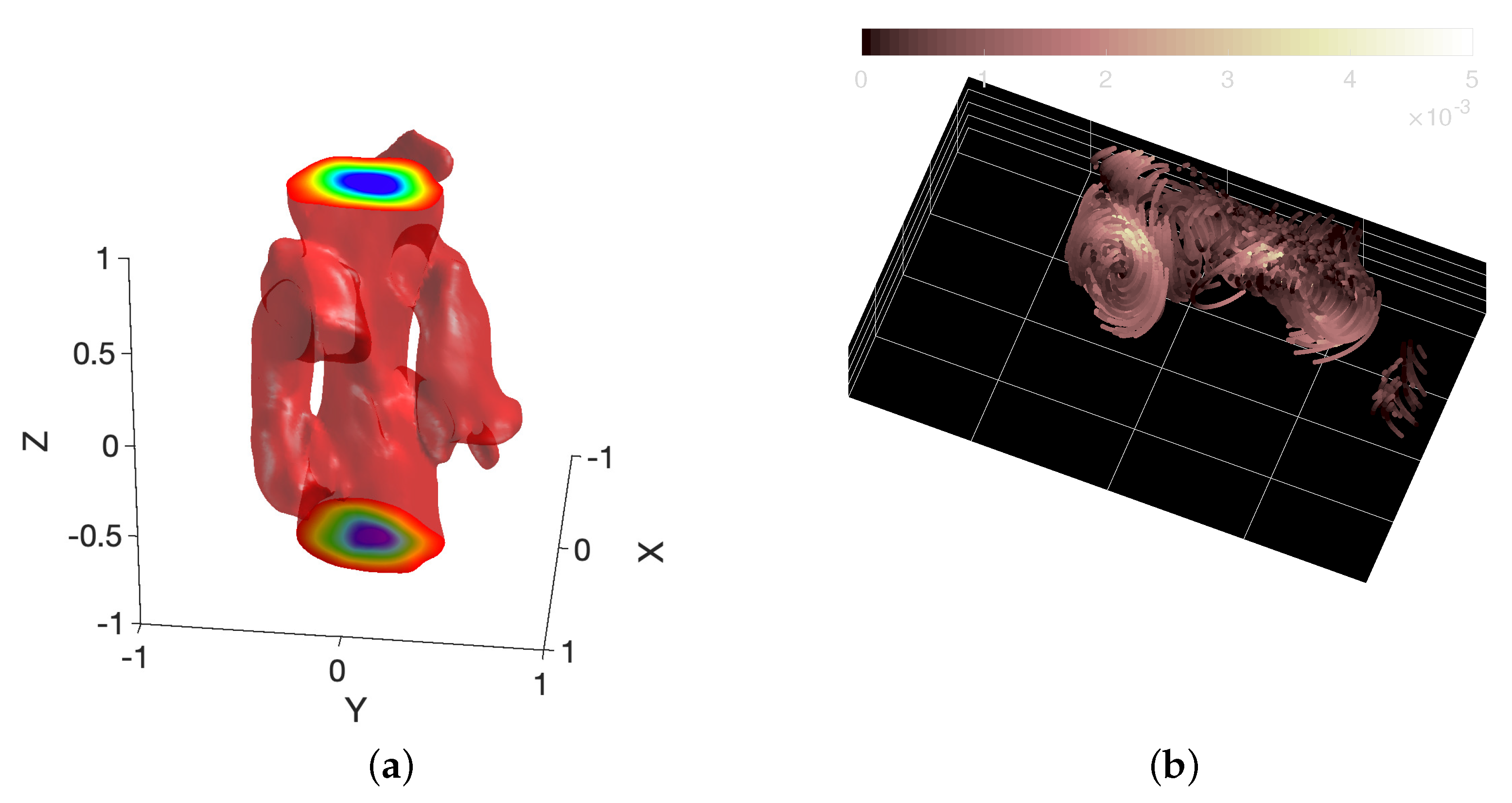
The most irregular structures of a given data set can be obtained by looking for places where the pseudo-Holder exponent takes its lowest value, and then analyzing the features of velocity and vorticity field around that place. This was done in [44] for DNS. In Figure 4d, we report a plot of the vorticity field in the experimental case. One sees that lower values of h are in the vicinity of (but do not coincide with) areas of large vorticities. More generally, one finds that the most irregular structures laying around places of lower h are vorticity filaments. The corresponding “typical” structure can be obtained by conditional averaging, after suitable translation and rotation [44]. It is shown in Figure 5a. It is an asymmetrical vorticity filament, with exponential vorticity profile corresponding to a Burgers vortex. Further investigation using time-resolved numerical [44] or experimental measurements [46] actually showed that the most irregular situations are obtained during vortex interaction, as illustrated in Figure 5b. More refined analysis prove that the interaction corresponds to vortex reconnection [47].
4. Link with Singularity
4.1. Fluctuating Dissipative Scale in the Multi-Fractal Framework
In its original version, Parisi and Frisch multi-fractal picture was based on the idea that the values of h were piloted by singularities of the Euler equation, that were regularized by viscosity at small enough scale. The scale at which this regularization occurs may be inferred from energetic arguments using Equation (40). Indeed, for a velocity field that is Hölder continuous with exponent h, we have that , while . The scale at which viscous dissipation becomes dominant with respect to the local energy transfers is there for . This scale also corresponds to the scale at which the local Reynolds number take a value of order unity, corresponding to a relaminarization of the flow [48]. For , we recover like for the Kolmogorov scale. Note that for , we have , so that the flow is never regularized. Locations where are thus only quasi-singuarities, while those with are genuine Navier–Stokes singularities. According to the constraint of Figure 3, we see that singularities are excluded for periodic boundary conditions, since cannot be reached. Most of astro- or geophysical flows have boundaries, however. What kind of singularities can we expect of this is the case? Is there a way we can give flesh to this intuition of Parisi and Frisch using observations?
4.2. Pressure Mediated Singularity
In 2014, Luo and Hou [49] provided a detailed numerical evidence of the existence of a finite-time blow up in an inviscid axisymmetric fluid with swirl. The flow is initially put into a kind of “differential rotation”, with the upper part of the tank rotating in one direction, and the lower part rotating in the other direction. The blow-up is characterized by a very strong increase of the amplitude of the vorticity, and occurs at the radial boundary and at the altitude of the shear layer. This blow-up was interpreted by Barkley [50] in terms of a “tea-cup like” singularity driven by the pressure field. This singularity mechanism is interesting because of the similarity of the geometry with a von Karman experiment, where the differential rotation is imparted by counter-rotating impellers [36]. It may then provide a suitable mechanism for building of singularities or quasi-singularities.
4.3. Singularity of Vortex Filaments
Another type of singularity can occur during vortex dynamics or interaction. Investigating such possibility with DNS or experiments is hard, and there is only limited evidence so far, for vortices starting perpendicular to each others [51,52]. Several simplified models however hints at a potential singularity.
4.3.1. Curvature Gradient Blow-Up
The first one is DLA: vortex filaments are modeled by one-dimensional lines with a given vorticity density. The line is allowed to move under the action of its own velocity field, computed using a Biot–Savart law, truncated at a given order. This provides the evolution of the curvature and the torsion of the vorticity line, as a function of time. Using the Hasimoto’s transformation [53] , one can map the corresponding equations to focusing non-linear Schrödinger equations for . The equation corresponding to the lowest order truncation was studied by Konopelchenko and Ortenzi [54]. They proved the existence of a finite-time blow-up, during which the gradient of the curvature and torsion becomes infinite, and the vorticity filaments undergo wild fluttering.
4.3.2. Reconnection Blow-Up
The previous “gradient catastrophe” scenario is interesting because large gradients curvature are typically observed during vortex reconnection, where “vorticity kinks” are built at early stages. Evidence of a singularity was actually observed in a simplified model of reconnection by Moffatt and Kimura [55,56]. In this model, vorticity filaments are also modeled by lines with constant vorticity density. Two filaments are initially placed at the ridges of a tetrahedra, and then allowed to interact via their mutual velocity field computed using the Biot–Savart law. The vortices interaction results in a self-similar evolution, with vorticity diverging as as the distance between the two filaments decreases as . There laws are exactly the laws that one would expect from scale symmetry argument of the viscid Navier–Stokes equation, that corresponds to a typical pseudo Holder exponent . It is not yet clear whether this blow-up scenario via reconnection is indeed present in Navier–Stokes, where interactions are more complex and self-regularizing mechanisms are present [57]. On the one hand, this blow-up scenario may explain why most irregular places are found near vortex interaction (see previous section). On the other hand, the value is forbidden by the properties of NSE (see Section 2.3.3), and no value of h lower than has ever been observed.
4.4. Singularity in the Complex Plane
Singularity Strip
A third possibility was initially proposed by Frisch and Morf [11]. It corresponds to a situation where the analytical continuation of the velocity field has complex branching points or poles that cross the real axis. This possibility is hard to investigate theoretically, because it is hard to establish the dynamics of those potential poles from the NSE. This has only be done for simpler 1D partial differential equations such as Burgers or KdV, using a technique invented by Calogero [58]. Forr example, Senouf et al. [59] found that the poles of Burgers equation with imaginary viscosity follow a Calogero dynamics, with logarithmic potential. The distance of the closest poles to the real axis is , while distance between poles on the imaginary axis is .
In more general cases, one can still try to follow numerically the fate of the poles that lay closest to the real axis, using the “singularity strip” method. This method is based on the observation that if the velocity field follows , with , then it Fourier transform satisfies:
The exponential decay of results in a similar exponential decay for the energy spectrum, over a typical distance . Monitoring the decay of the velocity spectrum therefore enables to measure the distance to the axis of the closest pole.
Such a method is simple to implement in theory, but difficult in practice because one needs to have a very good resolution to resolve the dissipative range and be able to have a reliable fit of the potential exponential decay.
This difficulty is illustrated in Figure 6a for the different spectra of Figure 1. One sees that one needs a very good resolution to be able to distinguish clear exponential decay, that shows up only when . For near unity, it may well be that the decay is in fact a stretched exponential [60], with exponent that may be close to the prediction by the renormalization group [60,61,62]. Given these caveats, one may try to infer the behaviour of the width of the singularity strip as a function of . This is shown in Figure 6b. One observes that the singularity strip width decays faster than the Kolmogorov length. Specifically, displays a power-law decay with exponent . Can we understand this value?
4.5. The Fluctuating Dissipation Scale and Correspondence Conjecture
A possible interpretation is the following, based on Frirsch and Morf [11] ideas, and on multi-fractal properties. Imagine that turbulence is characterized by a distribution of complex poles-that may dynamically interact following some sort of Calogero type of dynamics. The distance of these singularities to the real axis is , where i is the label corresponding to the pole. Around each pole, the velocity field behaves as , so that in the real space, (respectively ) behaves like a power-law with exponent (respectively ) over a distance from the real part of . In some sense, therefore acts as a local “cut-off”, that prevents formation of two large velocities (or velocity gradients). This notion is therefore similar to the local multi-fractal dissipative scale introduced in Section 4, and we may establish a correspondence . In that respect, at fixed , the distribution of is determined by the distribution of .
From the singularity strip method, we cannot determine the full distribution of , since the spectrum decay will be dominated by behaviour near the poles that is closest to the real axis, resulting in . Because it is the “most singular” point, it will correspond to the location where , the minimum Holder exponent in the set. We this get . Since , we finally get
For , as observed here, we thus get , close to what is observed in periodic DNS.
5. Conclusions
The multi-fractal framework invented by G. Parisi and U. Frisch proved to be a very powerful tool in incompressible 3D turbulence [63,64,65], both from the Eulerian [66] and Lagrangian point of view [67,68,69]. It should be viewed as a natural and general extension of the Kolmogorov theory. The adaptation of the global theory to geophysical flows is straightforward and very relevant, as already shown by Schertzer, Lovejoy and their collaborators [27,28,29]. To our knowledge, however, there has been no attempt to adapt the local theory to geophysical flows. Given the potential of such a framework to detect the most irregular structures, it would be certainly very illuminating to investigate the topological and dynamical properties of “most irregular areas” as defined by the local theory. Indeed, it may provide a physically based and statistically unbiased way to define “local extreme events”. Whether such events do correspond to local extreme events of societal interest (such as storms, heat waves, etc.) is an open question. I certainly hope that the present review will motivate research in that direction.
Funding
This work was funded by ANR TILT grant agreement no. ANR-20-CE30-0035, and ANR BANG grant agreement no. ANR-22-CE30-00xx.
Data Availability Statement
The data corresponding to the figures generated in this review can be obtained upon request to the author.
Acknowledgments
I thank A. Mailybaev for explaining the hidden scale symmetry to me and for very interesting discussions. I thank D. Buaria, J.-P. Laval, and F. Nguyen for giving me access to their DNS spectra, my students (F. Nguyen, P. Debue, D. Geneste, H. Faller) and post-docs (E-W. Saw, V. Valori, A. Cheminet) for all the work they shared with me, and my team members from EXPLOIT (J.-P. Laval, J.-M. Foucaut, Ch. Cuvier, F. Daviaud) for giving me access to the experimental data. This paper is dedicated to Uriel Frisch for its 80 (+2) birthday.
Conflicts of Interest
The author declares no conflict of interest.
References
- Grant, H.L.; Stewart, R.W.; Moilliet, A. Turbulence spectra from a tidal channel. J. Fluid Mech. 1962, 12, 241–268. [Google Scholar] [CrossRef]
- Kolmogorov, A.N. The local structure of turbulence in incompressible viscous fluids for very large Reynolds number. Dokl. Akad. Nauk SSSR 1941, 30, 913. [Google Scholar]
- Geneste, D.; Faller, H.; Nguyen, F.; Shukla, V.; Laval, J.P.; Daviaud, F.; Saw, E.W.; Dubrulle, B. About Universality and Thermodynamics of Turbulence. Entropy 2019, 21, 326. [Google Scholar] [CrossRef] [Green Version]
- Dubrulle, B.; Daviaud, F.; Faranda, D.; Marié, L.; Saint-Michel, B. How many modes are needed to predict climate bifurcations? Lessons from an experiment. Nonlinear Process. Geophys. 2022, 29, 17–35. [Google Scholar] [CrossRef]
- Batchelor, G.K.; Townsend, A.A. The nature of turbulent motion at large wave-numbers. Proc. R. Soc. Lond. Ser. Math. Phys. Sci. 1949, 199, 238–255. [Google Scholar] [CrossRef]
- Landau, L.; Lifshitz, L. Fluid Mechanics; Pergamon Press: London, UK, 1959. [Google Scholar]
- Kolmogorov, A.N. A refinement of previous hypotheses concerning the local structure of turbulence in a viscous incompressible fluid at high Reynolds number. J. Fluid Mech. 1962, 13, 82. [Google Scholar] [CrossRef] [Green Version]
- Frisch, U. Turbulence, the Legacy of A. N. Kolmogorov; Cambridge University Press: Cambridge, UK, 1996. [Google Scholar]
- Frisch, U.; Parisi, G. On the singularity structure of fully developed turbulence. In Proceedings of the Turbulence and Predictability in Geophysical Fluid Dynamics and Climate Dynamics; Gil, M., Benzi, R., Parisi, G., Eds.; Elsevier: Amsterdam, The Netherlands, 1985; pp. 84–88. [Google Scholar]
- Onsager, L. Statistical hydrodynamics. Il Nuovo Cimento (1943–1954) 1949, 6, 279–287. [Google Scholar] [CrossRef]
- Frisch, U.; Morf, R. Intermittency in nonlinear dynamics and singularities at complex times. Phys. Rev. A 1981, 23, 2673–2705. [Google Scholar] [CrossRef]
- Cheskidov, A.; Shvydkoy, R. Volumetric theory of intermittency in fully developed turbulence. arXiv 2022, arXiv:2203.11060. [Google Scholar]
- Mailybaev, A.A. Hidden scale invariance of intermittent turbulence in a shell model. Phys. Rev. Fluids 2021, 6, L012601. [Google Scholar] [CrossRef]
- Mailybaev, A.A. Hidden spatiotemporal symmetries and intermittency in turbulence. Nonlinearity 2022, 35, 3630–3679. [Google Scholar] [CrossRef]
- Mailybaev, A.A.; Thalabard, S. Hidden scale invariance in Navier-Stokes intermittency. Philos. Trans. R. Soc. Math. Phys. Eng. Sci. 2022, 380, 20210098. [Google Scholar] [CrossRef] [PubMed]
- Mailybaev, A.A. Solvable Intermittent Shell Model of Turbulence. Commun. Math. Phys. 2021, 388, 469–478. [Google Scholar] [CrossRef]
- Dubrulle, B.; Graner, F. Analogy between scale symmetry and relativistic mechanics. II. Electric analog of turbulence. Phys. Rev. E 1997, 56, 6435–6442. [Google Scholar] [CrossRef] [Green Version]
- Dubrulle, B. Anomalous Scaling and Generic Structure Function in Turbulence. J. Phys. II France 1996, 6, 1825–1840. [Google Scholar] [CrossRef] [Green Version]
- Dubrulle, B.; Graner, F. Possible Statistics of Scale Invariant Systems. J. Phys. II France 1996, 6, 797–816. [Google Scholar] [CrossRef]
- Dubrulle, B.; Graner, F. Scale Invariance and Scaling Exponents in Fully Developed Turbulence. J. Phys. II France 1996, 6, 817–824. [Google Scholar] [CrossRef]
- Graner, F.; Dubrulle, B. Analogy between scale symmetry and relativistic mechanics. I. Lagrangian formalism. Phys. Rev. E 1997, 56, 6427–6434. [Google Scholar] [CrossRef] [Green Version]
- Dubrulle, B.; Bréon, F.M.; Graner, F.; Pocheau, A. Towards an universal classification of scale invariant processes. Eur. Phys. J. Condens. Matter Complex Syst. 1998, 4, 89–94. [Google Scholar] [CrossRef]
- Pocheau, A. Scale invariance in turbulent front propagation. Phys. Rev. E 1994, 49, 1109–1122. [Google Scholar] [CrossRef]
- Dubrulle, B. Intermittency in fully developed turbulence: Log-Poisson statistics and generalized scale covariance. Phys. Rev. Lett. 1994, 73, 959–962. [Google Scholar] [CrossRef] [PubMed]
- She, Z.S.; Leveque, E. Universal scaling laws in fully developed turbulence. Phys. Rev. Lett. 1994, 72, 336–339. [Google Scholar] [CrossRef] [PubMed]
- She, Z.S.; Waymire, E.C. Quantized Energy Cascade and Log-Poisson Statistics in Fully Developed Turbulence. Phys. Rev. Lett. 1995, 74, 262–265. [Google Scholar] [CrossRef] [PubMed]
- Schertzer, D.; Lovejoy, S.; Schmitt, F.; Chigirinskaya, Y.; Marsan, D. Multifractal cascade dynamics and turbulent intermittency. Fractals 1997, 5, 427–471. [Google Scholar] [CrossRef]
- Schertzer, D.; Lovejoy, S. Non-Linear Variability in Geophysics, Scaling and Fractals; Kluwer: Dordrecht, The Netherlands, 1991. [Google Scholar]
- Schertzer, D.; Lovejoy, S. Multifractals, generalized scale invariance and complexity in Geophysics. Int. J. Bifurc. Chaos 2011, 21, 3417–3456. [Google Scholar] [CrossRef]
- Dubrulle, B.; Gibbon, J.D. A correspondence between the multifractal model of turbulence and the Navier-Stokes equations. Philos. Trans. R. Soc. Math. Phys. Eng. Sci. 2022, 380, 20210092. [Google Scholar] [CrossRef] [PubMed]
- Gibbon, J.D. Intermittency, cascades and thin sets in three-dimensional Navier-Stokes turbulence. EPL Europhys. Lett. 2020, 131, 64001. [Google Scholar] [CrossRef]
- Muzy, J.F.; Bacry, E.; Arneodo, A. Wavelets and multifractal formalism for singular signals: Application to turbulence data. Phys. Rev. Lett. 1991, 67, 3515. [Google Scholar] [CrossRef]
- Chevillard, L.; Castaing, B.; Lévêque, E.; Arneodo, A. Unified multifractal description of velocity increments statistics in turbulence: Intermittency and skewness. Phys. Nonlinear Phenom. 2006, 218, 77–82. [Google Scholar] [CrossRef] [Green Version]
- Faller, H.; Geneste, D.; Chaabo, T.; Cheminet, A.; Valori, V.; Ostovan, Y.; Cappanera, L.; Cuvier, C.; Daviaud, F.; Foucaut, J.M.; et al. On the nature of intermittency in a turbulent von Karman flow. J. Fluid Mech. 2021, 914, A2. [Google Scholar] [CrossRef]
- Iyer, K.P.; Sreenivasan, K.R.; Yeung, P.K. Scaling exponents saturate in three-dimensional isotropic turbulence. Phys. Rev. Fluids 2020, 5, 054605. [Google Scholar] [CrossRef]
- Dubrulle, B. Beyond Kolmogorov cascades. J. Fluid Mech. 2019, 867, P1. [Google Scholar] [CrossRef]
- Eyink, G.L. Turbulence Theory. Course Notes. The Johns Hopkins University. 2007–2008. Available online: http://www.ams.jhu.edu/eyink/Turbulence/notes/ (accessed on 12 October 2022).
- Bohr, T.; Rand, D. The entropy function for characteristic exponents. Phys. D Nonlinear Phenom. 1987, 25, 387–398. [Google Scholar] [CrossRef]
- Rinaldo, A.; Maritan, A.; Colaiori, F.; Flammini, A.; Rigon, R.; Rodriguez-Iturbe, I.; Banavar, J.R. Thermodynamics of fractal networks. Phys. Rev. Lett. 1996, 76, 3364. [Google Scholar] [CrossRef]
- Frisch, U.; Vergassola, M. A Prediction of the Multifractal Model: The Intermediate Dissipation Range. Europhys. Lett. (EPL) 1991, 14, 439–444. [Google Scholar] [CrossRef]
- Castaing, B.; Gagne, Y.; Marchand, M. Log-similarity for turbulent flows? Phys. D Nonlinear Phenom. 1993, 68, 387–400. [Google Scholar] [CrossRef]
- Chae, D. Nonexistence of Self-Similar Singularities for the 3D Incompressible Euler Equations. Commun. Math. Phys. 2007, 1, 203–215. [Google Scholar] [CrossRef] [Green Version]
- Nguyen, F.; Laval, J.P.; Kestener, P.; Cheskidov, A.; Shvydkoy, R.; Dubrulle, B. Local estimates of Holder exponents in turbulent vector fields. Phys. Rev. E 2019, 99, 053114. [Google Scholar] [CrossRef] [Green Version]
- Nguyen, F.; Laval, J.P.; Dubrulle, B. Characterizing most irregular small-scale structures in turbulence using local Hölder exponents. Phys. Rev. E 2020, 102, 063105. [Google Scholar] [CrossRef]
- Duchon, J.; Robert, R. Inertial energy dissipation for weak solutions of incompressible Euler and Navier-Stokes equations. Nonlinearity 2000, 13, 249. [Google Scholar] [CrossRef]
- Cheminet, A.E.A. Eulerian vs. Lagrangian irreversibility in an experimental turbulent swirling flow. Phys. Rev. Lett. 2022, 129, 124501. [Google Scholar] [CrossRef] [PubMed]
- Harekrishnan, A. Direct Numerical and Experimental Observation of Reconnection in a Turbulent Swirling Flow; University Paris Saclay, SPEC: Gif sur Yvette, France, 2022; to be submitted. [Google Scholar]
- Paladin, G.; Vulpiani, A. Degrees of freedom of turbulence. Phys. Rev. A 1987, 35, 1971–1973. [Google Scholar] [CrossRef] [PubMed]
- Luo, G.; Hou, T.Y. Potentially singular solutions of the 3D axisymmetric Euler equations. Proc. Natl. Acad. Sci. USA 2014, 111, 12968–12973. [Google Scholar] [CrossRef] [PubMed] [Green Version]
- Barkley, D. A fluid mechanic’s analysis of the teacup singularity. Proc. R. Soc. Math. Phys. Eng. Sci. 2020, 476, 20200348. [Google Scholar] [CrossRef]
- Ostilla-Mónico, R.; McKeown, R.; Brenner, M.P.; Rubinstein, S.M.; Pumir, A. Cascades and reconnection in interacting vortex filaments. Phys. Rev. Fluids 2021, 6, 074701. [Google Scholar] [CrossRef]
- Harekrishnan, A. (Warwick University, Coventry, UK). Private Communication, 2022. [Google Scholar]
- Hasimoto, H. A soliton on a vortex filament. J. Fluid Mech. 1972, 51, 477–485. [Google Scholar] [CrossRef]
- Konopelchenko, B.G.; Ortenzi, G. Gradient catastrophe and flutter in vortex filament dynamics. J. Phys. Math. Theor. 2011, 44, 432001. [Google Scholar] [CrossRef] [Green Version]
- Moffatt, H.K.; Kimura, Y. Towards a finite-time singularity of the Navier-Stokes equations Part 1. Derivation and analysis of dynamical system. J. Fluid Mech. 2019, 861, 930–967. [Google Scholar] [CrossRef] [Green Version]
- Moffatt, H.K.; Kimura, Y. Towards a finite-time singularity of the Navier-Stokes equations. Part 2. Vortex reconnection and singularity evasion. J. Fluid Mech. 2019, 870, R1, Corrigendum in J. Fluid Mech. 2020, 887, E2. [Google Scholar] [CrossRef] [Green Version]
- Buaria, D.; Pumir, A.; Bodenschatz, E. Self-attenuation of extreme events in Navier–Stokes turbulence. Nat. Commun. 2020, 11, 5852. [Google Scholar] [CrossRef]
- Calogero, F. Motion of poles and zeros of special solutions of nonlinear and linear partial differential equations and related solvable many-body problems. Il Nuovo Cimento B (1971–1996) 1978, 43, 177–241. [Google Scholar] [CrossRef]
- Senouf, D.; Caflisch, R.; Ercolani, N. Pole dynamics and oscillations for the complex Burgers equation in the small-dispersion limit. Nonlinearity 1996, 9, 1671–1702. [Google Scholar] [CrossRef]
- Buaria, D.; Sreenivasan, K.R. Dissipation range of the energy spectrum in high Reynolds number turbulence. Phys. Rev. Fluids 2020, 5, 092601. [Google Scholar] [CrossRef]
- Canet, L.; Rossetto, V.; Wschebor, N.; Balarac, G. Spatiotemporal velocity-velocity correlation function in fully developed turbulence. Phys. Rev. E 2017, 95, 023107. [Google Scholar] [CrossRef] [PubMed] [Green Version]
- Debue, P.; Kuzzay, D.; Saw, E.W.; Daviaud, F.m.c.; Dubrulle, B.; Canet, L.; Rossetto, V.; Wschebor, N. Experimental test of the crossover between the inertial and the dissipative range in a turbulent swirling flow. Phys. Rev. Fluids 2018, 3, 024602. [Google Scholar] [CrossRef] [Green Version]
- Benzi, R.; Paladin, G.; Parisi, G.; Vulpiani, A. On the multifractal nature of fully developed turbulence and chaotic systems. J. Phys. Math. Gen. 1984, 17, 3521–3531. [Google Scholar] [CrossRef]
- Boffetta, G.; Mazzino, A.; Vulpiani, A. Twenty-five years of multifractals in fully developed turbulence: A tribute to Giovanni Paladin. J. Phys. Math. Theor. 2008, 41, 363001. [Google Scholar] [CrossRef] [Green Version]
- Meneveau, C.; Sreenivasan, K.R. The multifractal nature of turbulent energy dissipation. J. Fluid Mech. 1991, 224, 429–484. [Google Scholar] [CrossRef]
- Chevillard, L.; Roux, S.G.; Lévêque, E.; Mordant, N.; Pinton, J.F.; Arnéodo, A. Intermittency of Velocity Time Increments in Turbulence. Phys. Rev. Lett. 2005, 95, 064501. [Google Scholar] [CrossRef] [Green Version]
- Borgas, M.S. The multifractal lagrangian nature of turbulence. Philos. Trans. R. Soc. Lond. Ser. Phys. Eng. Sci. 1993, 342, 379–411. [Google Scholar] [CrossRef]
- Biferale, L.; Boffetta, G.; Celani, A.; Devenish, B.J.; Lanotte, A.; Toschi, F. Multifractal Statistics of Lagrangian Velocity and Acceleration in Turbulence. Phys. Rev. Lett. 2004, 93, 064502. [Google Scholar] [CrossRef] [PubMed] [Green Version]
- Arnèodo, A.; Benzi, R.; Berg, J.; Biferale, L.; Bodenschatz, E.; Busse, A.; Calzavarini, E.; Castaing, B.; Cencini, M.; Chevillard, L.; et al. Universal Intermittent Properties of Particle Trajectories in Highly Turbulent Flows. Phys. Rev. Lett. 2008, 100, 254504. [Google Scholar] [CrossRef] [PubMed]
Figure 1.
Hierarchy of turbulence (a) Vortices of all sizes in the South Atlantic Ocean on 5 January 2021. Vortices are visualized by phytoplankton blooms (shown in green and light blue). Image Credit: NASA/Goddard Space Flight Center Ocean Color/NOAA-20/NASA-NOAA Suomi NPP. (b) K41 Spectrum computed from ocean measurements ([1], blue diamonds) and DNS at between 52 and 650 (colored lines). Insert: multi-fractal universal representation of the spectrum, with .

Figure 2.
Test of universality using structure function based on wavelet transform. (a) K41 universality, given by Equation (3); (b) multi-fractal universality, given by Equation (35). DNS are shown with open symbols, while experiments are shown with filled symbols. The structure functions have been shifted by arbitrary factors for clarity and are coded by color: : blue symbols; : red symbols; : orange symbols; : magenta symbols; : green symbols; : light blue symbols; : dark red symbols; : blue symbols; : red symbols. Note that on that graph, the symbols are hidden behind the symbols, because both have very weak intermittency. For K41 universality to hold, all the function should be constant with p, with a level depending on p. The dashed lines are power laws with exponents . Figure adapted from Geneste et al. [3].

Figure 3.
Empirical multi-fractal spectrum computed from data using different definitions of . (a) using velocity increments in high resolution DNS [35]: magenta: transverse velocity increments; green: longitudinal velocity increments. Blue dotted lines is a log-Poisson fit.; (b) using wavelet coefficients and the universal curves in Figure 2b. Red: data points. Blue dotted lines is a log-normal (parabolic) fit. The black lines delineate the admissibility range of the multi-fractal spectrum in three dimensions, obtained by theory. The zone left of the vertical dotted line is excluded as a result of Equation (29). The zone below the horizontal continuous line is excluded as a result of normalization of [36]. The zone below the black dashed-dotted line is excluded as a result of both Equation (29) and the four-fifths law.

Figure 4.
Local Holder exponents for experimental data at resolution . (a) Map of local Holder exponent. (b) Histogram of values of h in the field of view (a). Most of the values are above but there are a few events where , meaning non-differentiability. Note that for , the field is not twice differentiable, meaning we cannot define a dissipation. (c) Local-energy transfer for the velocity field corresponding to (a). (d) Vorticity field corresponding to (a).

Figure 5.
(a) Typical vorticity structure found near location of smallest local Holder exponent, obtained by averaging several structure after suitable re-orientation. Note the presence of two pieces of bent filaments on either side of the structure. This is a remnant of the reconnection event. (b) Example of a reconnection event captured in the experimental von Karman device by selecting of trajectories obtained around a very irregular point. The trajectories are coded by velocity norm (in m s, with intensity given by the colorbar.

Figure 6.
(a) Compensated energy spectrum vs. in the dissipative range for DNS at to 650, where the color codes the Reynolds number, and with color code providedin panel (b). The plot is in log-lin so that a straight line corresponds to an exponential decay. The area where this is satisfied is delimited on each case via yellow symbols. The fit is materialized by a black line. (b) Non-dimensional width of the singularity strip 2 as a function of . The black dotted line is corresponds to a power-law .


Table 1.
Summary of the analogy between the multi-fractal formalism of turbulence and relativity. We have set the origin of the axis to 0 for simplicity.
Table 1.
Summary of the analogy between the multi-fractal formalism of turbulence and relativity. We have set the origin of the axis to 0 for simplicity.
| Relativity | Multi-Fractal | |
|---|---|---|
| Time | T | |
| Space | X | |
| Speed | ||
| Group structure | velocity composition | relative exponent composition |
| Limiting speed(s) | c | and |
Table 2.
Summary of the analogy between the multi-fractal formalism of turbulence and thermodynamics.
Table 2.
Summary of the analogy between the multi-fractal formalism of turbulence and thermodynamics.
| Thermodynamics | Turbulence | |
|---|---|---|
| Temperature | ||
| Energy | E | |
| Entropy | S | , |
| Number of d.f. | N | |
| Volume | V | |
| Free energy | F |
Publisher’s Note: MDPI stays neutral with regard to jurisdictional claims in published maps and institutional affiliations. |
© 2022 by the author. Licensee MDPI, Basel, Switzerland. This article is an open access article distributed under the terms and conditions of the Creative Commons Attribution (CC BY) license (https://creativecommons.org/licenses/by/4.0/).
Share and Cite
MDPI and ACS Style
Dubrulle, B. Multi-Fractality, Universality and Singularity in Turbulence. Fractal Fract. 2022, 6, 613. https://doi.org/10.3390/fractalfract6100613
AMA Style
Dubrulle B. Multi-Fractality, Universality and Singularity in Turbulence. Fractal and Fractional. 2022; 6(10):613. https://doi.org/10.3390/fractalfract6100613
Chicago/Turabian StyleDubrulle, Bérengère. 2022. "Multi-Fractality, Universality and Singularity in Turbulence" Fractal and Fractional 6, no. 10: 613. https://doi.org/10.3390/fractalfract6100613