Figure 2.
The 2-faced web network .
Figure 2.
The 2-faced web network .
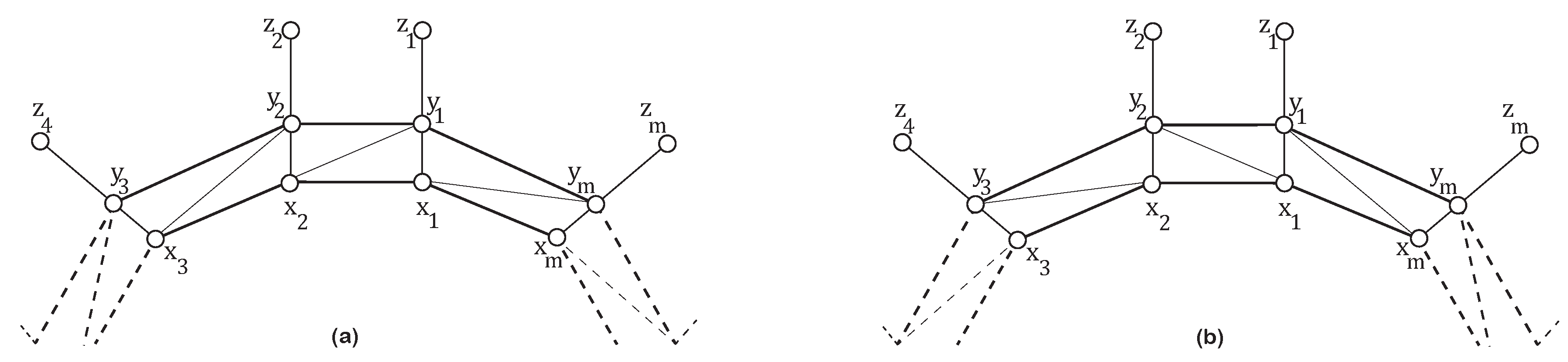
Figure 3.
Possible 3-faced web networks (a) (b) (right).
Figure 3.
Possible 3-faced web networks (a) (b) (right).
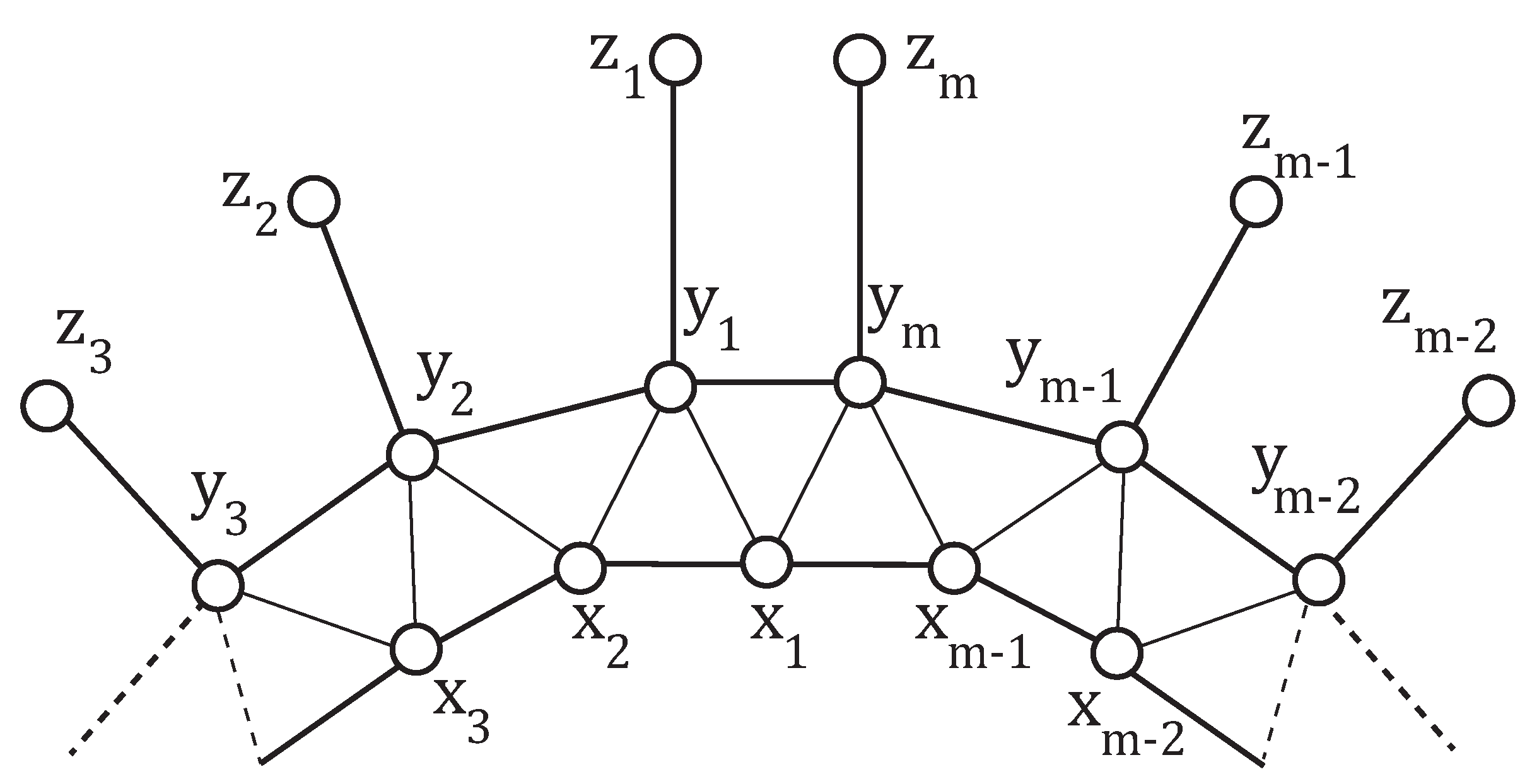
Figure 4.
Antiprism Web Network .
Figure 4.
Antiprism Web Network .
Figure 5.
Graphical analysis, 2D (left) and 3D (right).
Figure 5.
Graphical analysis, 2D (left) and 3D (right).
Table 1.
RNs for .
Table 1.
RNs for .
| RNs | Cardinalities |
|---|
| ,,, | |
| ,,,, | |
| |
| |
| |
| |
| |
| |
| |
| |
Table 2.
RNs for .
Table 2.
RNs for .
| RNs | Cardinalities |
|---|
| ,,,,,,, | |
| |
| |
| |
Table 3.
RNs for .
Table 3.
RNs for .
| RNs | Cardinalities |
|---|
| |
| , ,,, | |
| , | |
| |
| |
| |
| |
| |
Table 4.
RNs for .
Table 4.
RNs for .
| RNs | Cardinalities |
|---|
| |
| |
| |
| |
| |
Table 5.
RNs for .
Table 5.
RNs for .
| RNs | Cardinalities |
|---|
| , | |
| ,,, | |
| , | |
| |
| |
| |
Table 6.
RNs for .
Table 6.
RNs for .
| RNs | Cardinalities |
|---|
| |
| |
| |
| |
Table 7.
RNs for .
Table 7.
RNs for .
| RNs | Elements |
|---|
| |
| |
| |
| |
| |
| |
| |
| |
| |
Table 8.
RNs for .
Table 8.
RNs for .
| RNs | Elements |
|---|
| |
| |
| |
Table 9.
RNs for .
Table 9.
RNs for .
| RNs | Elements |
|---|
| |
| |
| |
Table 10.
RNs for and .
Table 10.
RNs for and .
| RNs | Elements |
|---|
| |
Table 11.
RNs for .
Table 11.
RNs for .
| RNs | Elements | Equality |
|---|
| | , |
| | , |
| | , |
Table 12.
RNs for .
Table 12.
RNs for .
| RNs | Elements | Equality |
|---|
| | |
| | |
| | |
| | |
| | |
| | |
| | |
| | |
| | |
| | |
| | |
| | |
| | |
| | |
| | |
| | |
| | |
| | |
| | |
| | |
| | |
| | , |
| | , |
| | , |
Table 13.
RNs for .
Table 13.
RNs for .
| RNs | Elements |
|---|
| |
| |
| |
| |
| |
| |
| |
| |
| |
Table 14.
RNs for .
Table 14.
RNs for .
| RNs | RNs | Elements |
|---|
| | |
| | |
| | |
Table 15.
RNs for .
Table 15.
RNs for .
| RNs | Elements |
|---|
| |
| |
| |
Table 16.
RNs for .
Table 16.
RNs for .
| RNs | Elements |
|---|
| |
| |
| |
| |
| |
| |
Table 17.
RNs for .
Table 17.
RNs for .
| RNs | Elements |
|---|
| |
| |
| |
Table 18.
RNs for .
Table 18.
RNs for .
| RNs | Elements |
|---|
| |
| |
| |
Table 19.
RNs for .
Table 19.
RNs for .
| RNs | Elements | Equality |
|---|
| | , |
| | , |
| | , |
Table 20.
RNs for .
Table 20.
RNs for .
| RNs | Elements | Equality |
|---|
| | |
| | |
| | |
| | |
| | |
Table 21.
RNs for .
Table 21.
RNs for .
| RNs | Elements |
|---|
| |
| |
| |
Table 22.
RNs for .
Table 22.
RNs for .
| RNs | Elements |
|---|
| |
| |
| |
Table 23.
RNs for .
Table 23.
RNs for .
| RNs | Elements |
|---|
| |
| |
| |
Table 24.
RNs for .
Table 24.
RNs for .
| RNs | Elements |
|---|
| |
| |
| |
| |
| |
| |
Table 25.
RNs for .
Table 25.
RNs for .
| RNs | Elements | Equality |
|---|
| | |
| | |
| | |
| | |
| | |
| | |
| | |
Table 26.
RNs for .
Table 26.
RNs for .
| RNs | Elements |
|---|
| |
| |
| |
Table 27.
RNs for .
Table 27.
RNs for .
| RNs | Elements |
|---|
| |
Table 28.
RNs for .
Table 28.
RNs for .
| LRNs | Elements |
|---|
| |
| |
| |
Table 29.
LRNs for .
Table 29.
LRNs for .
| LRNs | Elements |
|---|
| |
| |
| |
Table 30.
LRNs for .
Table 30.
LRNs for .
| LRNs | Elements |
|---|
| |
| |
| |
Table 31.
LRNs for .
Table 31.
LRNs for .
| LRNs | Elements |
|---|
| |
Table 32.
RNs for .
Table 32.
RNs for .
| RNs | Elements |
|---|
| |
| |
| |
| |
| |
| |
Table 33.
RNs for .
Table 33.
RNs for .
| RNs | Elements |
|---|
| |
| |
| |
Table 34.
RNs for .
Table 34.
RNs for .
| RNs | Elements | Equality |
|---|
| | |
| | |
| | |
| | |
| | |
| | |
Table 35.
RNs for .
Table 35.
RNs for .
| RNs | Elements | Equality |
|---|
| | |
| | |
| | |
Table 36.
RNs for .
Table 36.
RNs for .
| RNs | Elements | Equality |
|---|
| | |
| | |
| | |
Table 37.
RNs for .
Table 37.
RNs for .
| RNs | Elements |
|---|
| |
Table 38.
LRNs for .
Table 38.
LRNs for .
| LRNs | Elements |
|---|
| |
| |
| |
| |
| |
| |
Table 39.
LRNs for .
Table 39.
LRNs for .
| LRNs | Elements |
|---|
| |
| |
| |
Table 40.
LRNs for .
Table 40.
LRNs for .
| LRNs | Elements |
|---|
| |
| |
| |
Table 41.
LRNs for .
Table 41.
LRNs for .
| LRNs | Elements |
|---|
| |
Table 42.
Summarized Numerical Results.
Table 42.
Summarized Numerical Results.
| | | | | Remarks |
|---|
| | 1 | | 1 | Bounded and Constant |
| | 1 | 3 | 1 | Bounded and Constant |
| | | 2 | 2 | Bounded and Constant |
| | | 2 | 2 | Bounded and Constant |
| | | 2 | 2 | Bounded and Constant |


 ,
, 


