Article

Control and Robust Stabilization at Unstable Equilibrium by Fractional Controller for Magnetic Levitation Systems

by
Banu Ataşlar-Ayyıldız
*,
Oğuzhan Karahan
and
Serhat Yılmaz
Department of Electronics and Communication Engineering, Kocaeli University, Kocaeli 41001, Turkey
*
Author to whom correspondence should be addressed.
Fractal Fract. 2021, 5(3), 101; https://doi.org/10.3390/fractalfract5030101
Submission received: 9 July 2021 / Revised: 12 August 2021 / Accepted: 17 August 2021 / Published: 20 August 2021
(This article belongs to the Special Issue Fractional Order Systems and Their Applications)

Abstract

:
The problem of control and stabilizing inherently non-linear and unstable magnetic levitation (Maglev) systems with uncertain equilibrium states has been studied. Accordingly, some significant works related to different control approaches have been highlighted to provide robust control and enhance the performance of the Maglev system. This work examines a method to control and stabilize the levitation system in the presence of disturbance and parameter variations to minimize the magnet gap deviation from the equilibrium position. To fulfill the stabilization and disturbance rejection for this non-linear dynamic system, the fractional order PID, fractional order sliding mode, and fractional order Fuzzy control approaches are conducted. In order to design the suitable control outlines based on fractional order controllers, a tuning hybrid method of GWO–PSO algorithms is applied by using the different performance criteria as Integrated Absolute Error (IAE), Integrated Time Weighted Absolute Error (ITAE), Integrated Squared Error (ISE), and Integrated Time Weighted Squared Error (ITSE). In general, these objectives are used by targeting the best tuning of specified control parameters. Finally, the simulation results are presented to determine which fractional controllers demonstrate better control performance, achieve fast and robust stability of the closed-loop system, and provide excellent disturbance suppression effect under nonlinear and uncertainty existing in the processing system.

1. Introduction

For the purpose of weakening the bulky friction problem in mechanical contact connecting both stationary and active parts in the system, magnetically levitated (Maglev) technology is used for eliminating this mechanical contact. Thus, the position of the levitated object can be effectively adjusted and also the stiffness of the Maglev system can be changed. For that reason, the most outstanding works have been found to be related to the Maglev technology in a wide range of applications such as magnetic bearings [1], high speed magnetic levitation trains [2,3], vibration isolation [4], aircraft take-off and landing [5], analysis of forensic evidence, minerals and internal defects in plastic gears [6,7,8], microelectromechanical systems [9], and disease diagnostic [10].
Since the Maglev system has non-linear dynamic characteristics and is also inherently unstable, achieving stability and dynamic tracking performance while controlling the position of the levitated object is a challenging task. In the literature, many studies report suitable control strategies in order to control the position of the levitated object for achieving better dynamic system response. Among different control strategies, Proportional–Integral-Derivative (PID) and Linear Quadratic Regulator (LQR) controllers, which are the basic linear control techniques, have been proposed by researchers for the Maglev system. Yaseen [11] employed these controllers to examine the stability analysis of the Maglev control system in the presence of disturbances. In addition, the many experiments were conducted for showing the superiority of which controller and comparing the controllers in terms of providing more stability. Zhu et al. [12] designed a simple PID controller for achieving good tracking performance of the Maglev system. However, when applied to the Maglev system under high disturbance, the controlled system usually could not exhibit satisfactory performance. To overcome this matter, Ghosh et al. [13] proposed a two degree of freedom (2-DOF) PID controller for implementing the Maglev system. Moreover, the PID controller was applied to the system for comparison in terms of superior robustness. Acharya et al. [14] designed a 2-DOF PID controller for stabilizing a Maglev system with time delay. However, in order to obtain the best system response, it is important to optimally tune the controller parameters. Therefore, in that paper, the optimal values of the parameters were identified by using symbiotic organisms search (SOS) algorithm. Also, to show the advantage of the proposed controller, the 1-DOF PID controller was optimized and their performances were compared as simulation results.
Apart from PID controllers, the presence of fractional order PID (FOPID) controllers have been found in the literature to provide more design flexibility and more capable under uncertainty and disturbances. The FOPID controller, which is introduced by Podlubny in 1994 [15], is a control application of the fractional calculus where the orders of derivatives and integrals are non-integer. This controller is characterized by three gains (the proportional, integral and derivative) and two order parameters (the integrating order and the derivative order, λ and μ , respectively). Consequently, the PID controllers are extended to the FOPID controllers by using two additional fractional order parameters ( μ and λ ) and better performance can be provided.
The concept of the FOPID controller in improving the transient response of the Maglev system was presented by Demirören et al. [16]. In their paper, the authors proposed an improved optimization algorithm to update the parameters of the FOPID controller. Also, the performance of the Maglev system with the optimized FOPID controller was examined through transient response and frequency response analyses. In another paper, using both ant colony optimization (ACO) algorithm and the Ziegler–Nichols technique, an FOPID controller was designed by Mughees and Mohsin [17] for the Maglev system. Moreover, for comparative analysis, in that paper, the results obtained with FOPID controller were compared with that of PID controller for illustrating highly efficient results. A FOPID controller of the Maglev system was designed based on four different performance indexes by Bauer and Baranowski [18] through two methods—Nyquist stability criteria and Simulated Annealing algorithm. In their paper, experiments were performed to validate the robustness of the designed controllers and also the methods were compared under external disturbances for the stability analysis of the Maglev system with designed controllers. On the other hand, as a result of putting forward the concept of 2-DOF controller, a realization of the 2-DOF FOPID control technique was addressed by Swain et al. [19] for the Maglev system. Moreover, the proposed 2-DOF FOPID controller was compared to its integer order counterpart in terms of superior response and robustness. One of the other ways of implementing the fractional order 2-DOF controller was realized by Acharya and Mishra [20] while tuning the controller with the proposed optimization algorithm for achieving the required closed-loop performance of the Maglev system. A different design of the 2-DOF FOPID controller was proposed by Pandey et al. [21] and applied to the Maglev system for stabilizing the system. As a result, the detailed investigation has been given in [22] for controlling the Maglev system based on 1 & 2-DOF integer order and fractional order PID controllers by tuning with the optimization algorithms according to the different performance criteria.
Due to the low sensitivity to variations in system parameters, external disturbances, and nonlinear dynamics, one of the robust controller designs which try to solve these transient stability problems can be considered as a sliding mode control (SMC). The SMC method has attracted much attention in designing disturbance rejection tracking control for the Maglev system, especially attenuating the effect of various uncertainties and external disturbances. Starbino and Sathiyavathi [23] designed SMC for achieving the desired ball position of the Maglev system under model uncertainties and disturbance. Moreover, for comparing the performances of the PID controller and SMC, simulation and physical implementation were conducted based on servo and different trajectories, and disturbance rejection and robustness test. In their paper, the control performance of the presented controllers was illustrated by comparing the transient response characteristics and the values of ISE and IAE for both PID and SMC. Shieh et al. [24] developed a robust optimal SMC approach for position tracking of the Maglev system in terms of robustness to parametric uncertainties. On the other hand, many researchers have constructed advanced controllers by using intelligent control techniques such as neural networks and fuzzy system. For the purpose of controlling the ball position of the Maglev system, an intelligent SMC approach was proposed by Lin et al. [25] by using a radial basis function network. Moreover, for verifying the effectiveness of the proposed controller, some experiments were performed. In another work for the satisfactory tracking performance of the Maglev system, an adaptive recurrent neural network intelligent SMC was designed by Chen and Kuo [26]. Also, by illustrating the validity of the proposed controller, SMC and PID, some experimental results were compared in that paper. Besides, using an adaptive technique, a fast terminal SMC approach was developed by Boonsatit and Pukdeboon [27] for achieving fast response and high accuracy of the Maglev system.
For the purpose of enhancing the chattering problem and improving the dynamic response of the closed-loop controlled Maglev system, taking advantage of fractional order calculus, the fractional order can be included into the design of SMC. Roy and Roy [28] studied the detailed comparative analysis between SMC and FOSMC applied to position control of the Maglev system in terms of tracking accuracy, assessing transient response, and the improvement of control effect and energy. Pandey et al. [29] developed fractional order integral dynamic sliding mode controllers for reducing the control effort and increasing the robustness of the Maglev system under parameter uncertainties. For achieving good control performance and reducing the tracking error and chattering effect, Wang et al. [30] designed a new FOSMC for the Maglev system with fractional order. In another work, for reducing the chattering in the SMC, a hybrid control approach based on combination of the SMC and fuzzy control was proposed by Zhang et al. [31] for the control of the Maglev system. The PSO was utilized for tuning the parameters of the SMC using the exponential reaching law method. From the simulation and experiments, it could be inferred that the proposed control approach exhibits robust performance under the disturbances and reduces chattering effectively.
Control of the nonlinear process is more challenging, especially disturbance rejection and no sensitivity to parameter variations as compared to that of a linear process. For the purpose of overcoming this challenge, soft computing techniques such as fuzzy logic, neural network, neuro-fuzzy etc. have been increasingly investigated. Among these, the use of fuzzy logic as computational intelligence-dependent designed control method has been recently developed, and is popular and widely used in control systems. The main motivation of the researchers has been the use of a combination of popular and easily applicable in practice methods such as Takagi-Sugeno fuzzy systems and PID control to design different class of fuzzy PID controllers that ensure sufficient control performance. So as to enhance the performance of a PID controlled Maglev system, by using a fuzzy inference system for self-regulating PID controller parameters, a fuzzy PID compound controller was designed in [32,33,34] for stabilizing the operation of the Maglev system. Sahoo et al. [35] focused on control of a real time Maglev system identified based on the teaching-learning based optimization-based functional link artificial neural network (FLANN). Moreover, the control of this real Maglev and the identified model was performed with the fuzzy PID controller. In that paper, the response of the identified Maglev system controlled by fuzzy PID control was compared with that of the fuzzy PID controlled actual one. Burakov [36] developed a fuzzy PID controller using the genetic algorithm (GA) for controlling the Maglev system. An incremental PID control approach based on fuzzy logic inference was proposed by Ataşlar–Ayyıldız and Karahan [37] for reducing the control effort and enhancing the control accuracy of the Maglev system. In the paper, by combining a fuzzy control approach with PID control approach, a fuzzy PID controller was designed by using the CS algorithm and also compared with the tuned PID and FOPID controllers. Moreover, to show the superiority of the proposed controller, the simulations and comparisons were performed in the presence of different operation conditions. In another work, modelling of three-input fuzzy PID controller was realized by Sain and Mohan [38] for controlling the unstable nonlinear Maglev system. In the paper, the parameters of the proposed fuzzy PID controller were optimized with GA based on the cost function, including the error and control effort. Moreover, the responses of the closed loop Maglev system with the PID and proposed fuzzy PID controllers were illustrated and compared in terms of the cost value, IAE, ISE, and control signal. In another study of the same authors, considering fractional order calculus, the fractional order was included into a new type of fuzzy PID controller proposed by the authors in order to perform the real-time control of the same Maglev system [39]. The controller parameters for the fuzzy PID and fractional fuzzy PID were also tuned by GA based on the same cost function. In the paper, the closed-loop performances of the Maglev controlled with the proposed controllers were demonstrated and compared according to the control signal, time domain integral error indices, and the cost function value.
The literature survey given above evinces that various control approaches have been proposed for the Maglev system and it is also revealed that the performance of the Maglev system depends on mainly the structure of the controller and its optimization technique. In the light of this information, in this paper, the main aim of this study is to experiment with different controllers based on fractional order calculus such as FOPID, FOSMC, and FOFPID tuned by the GWO–PSO algorithm in order to reach the optimum dynamic response of the Maglev system under parametric uncertainties and disturbances.
The main objectives and contributions of this study are itemized as follows:
  • To design and investigate the roles of the FOFPID controller in a Maglev system;
  • To use the GWO–PSO algorithm in designing process of the FOFPID controller considering its optimization for the first time in the literature and due to short computation time of the algorithm;
  • To illustrate the advantage of GWO–PSO-based FOFPID over FOPID and FOSMC tuned by the GWO–PSO algorithm for the Maglev system;
  • To validate the superiority of the presented fractional order controllers compared to the integer order counterparts proposed in the literature like PID and SMC for the above stated system;
  • To scrutinize the results based on dynamic transient responses of the fractional order controllers tuned according to the IAE, ISE, ITAE, and ITSE;
  • To carry out sensitivity analysis for assessing the robustness of the designed fractional order controllers in the presence of parameter uncertainty, external disturbance, and different trajectory tracking.
The organization of the article is as follows. The mathematical model of the Maglev system is described in Section 2. The structures of the FOPID, FOSMC, and FOFPID controllers are presented in Section 3. The GWO–PSO algorithm is given in Section 4. The simulation results are given in Section 5. Finally, the concluding remarks are given in Section 6.

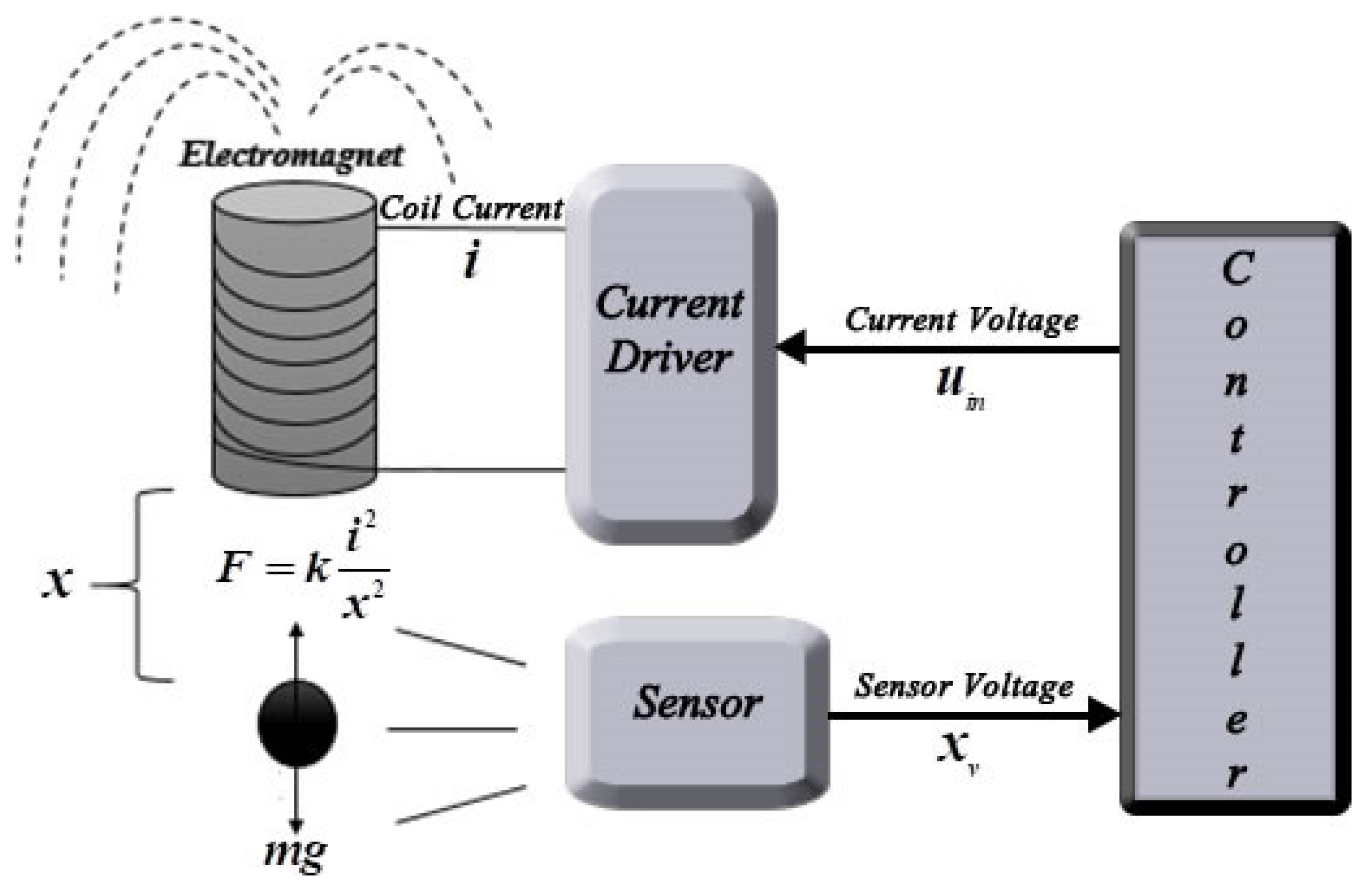
2. Mathematical Model of the Maglev System

The schematic of the Maglev system used is shown in Figure 1, which is the experimental setup implemented in [23]. The mathematical model of the system, related to the ball position x ( t ) and the electromagnet coil current i ( t ) , is given by [23]:
m x ¨ = m g + k i 2 x 2
where m is the mass of the levitated object, which is a ferromagnetic ball, g is the acceleration due to gravity, and k is an electromechanical conversion constant. At the equilibrium point ( x 0 , i 0 ), the value of k is obtained as follows:
k = m g x 0 2 i 0 2
Then, by linearizing this nonlinear model about the equilibrium point, the transfer function is obtained as below:
X ( s ) I ( s ) = 2 g i 0 2 s 2 2 g x 0
Since the coil current i ( t ) is proportional to the input voltage u i n ( t ) i.e., u i n ( t ) = K a i ( t ) , and the output of sensor x v ( t ) is proportional to the position of the ball x ( t ) , i.e., x v ( t ) = K s x ( t ) , the transfer function from u i n ( t ) to x v ( t ) is obtained as:
X v ( s ) U i n ( s ) = K s K a s 2 2 g x 0
Finally, by substituting system parameters given in [23] (reported in Table 1) into Equation (4), the transfer function is determined as below:
G ( s ) = 2502.96 s 2 981.511
By introducing x 1 ( t ) = x v ( t ) and x 2 ( t ) = x ˙ v ( t ) as states, and y ( t ) = x v ( t ) as output, the state space model of the system is obtained as:
x ˙ ( t ) = [ 0 1 981.511 0 ] x ( t ) + [ 0 2502.96 ] u i n ( t ) y ( t ) = [ 1 0 ] x ( t )

3. Controllers’ Design

The principles of the proposed methodology to design Fractional Order PID (FOPID) Controller, Fractional Order Sliding Mode Control (FOSMC), and Fractional Order Fuzzy PID (FOFPID) controllers will be presented in the subsequent subsections.

3.1. Conventional and Fractional Order PID Controller

A conventional PID controller has three parameters K p , K i and K d , with the transfer function:
C P I D ( s ) = K p + K i 1 s + K d s
As compared to the conventional PID controller, fractional order PID controller introduces two additional adjustable parameters λ and µ. These parameters are non-integer orders of derivative and integral, respectively. The differential equation of the FOPID controller is given as the following [40]:
u ( t ) = K p e ( t ) + K i D t λ 0 e ( t ) + K d D t μ 0 e ( t )
where D t α 0 is the fractional calculus operator, which will be explained in detail in Section 3.4, and e ( t ) is the error signal corresponding the difference between desired position and the actual ball position. Let r ( t ) and r v ( t ) be the reference signal in meter and corresponding sensor output in volts, respectively. Hence, the error signal is defined as the difference between r v ( t ) and x v ( t ) .
According to Equation (8), the transfer function of FOPID controller is obtained as [40,41,42]:
C F O P I D ( s ) = K p + K i 1 s λ + K d s μ

3.2. Integer Order and Fractional Order Sliding Mode Control

The objective of the controller design by using the Sliding Mode Control methodology is to make the system output track the reference by choosing a sliding surface in the error space [42]. For the MAGLEV system considered in this study, the convergence of sliding variable to zero will ensure x v ( t ) = r v ( t ) .
In this study, a fractional-order sliding surface based approach is used for the Fractional Order SMC. For fractional-order derivative and integration, the fractional calculus operator ( D t α 0 ) explained in details in Section 3.4 is used.
Let the sliding surface, S f ( t ) , be defined as [27,28,29,43]:
S f ( t ) = c 1 D t α 0 e ( t ) + c 2 e ( t )
where c 1 ,   c 2 > 0 are the tuning parameters, which determine the slope of sliding manifold and e ( t ) is tracking error, as mentioned in the previous subsection, defined as the difference between the desired position and the actual ball position in volts:
e ( t ) = r v ( t ) x v ( t )
From Equation (10), the derivative of S f ( t ) is:
S ˙ f ( t ) = c 1 D t α 0 e ˙ ( t ) + c 2 e ˙ ( t )
S ˙ f ( t ) = c 1 D t α 1 0 e ¨ ( t ) + c 2 e ˙ ( t )
where the first and the second derivative of e ( t ) are obtained from Equation (11), as below:
e ˙ ( t ) = x ˙ v ( t ) = x ˙ 1 ( t ) = x 2 ( t )
e ¨ ( t ) = x ˙ 2 ( t ) = a 21 x 1 ( t ) b 2 u i n ( t )
In here, a 21 = 981.511 is the element in the first column of the second row of the system dynamic matrix, and b 2 = 2502.96 is the element in the second row of the system input matrix in Equation (6).
By replacing e ¨ ( t ) with the equality in Equation (15), the first derivative of S f ( t ) is obtained as [28,29,43]:
S ˙ f ( t ) = c 1 D t α 1 0 ( a 21 x 1 ( t ) b 2 u i n ( t ) ) + c 2 e ˙ ( t )
In order to derive the equivalent control input u e q ( t ) , the first derivative of the sliding surface is made to S ˙ f ( t ) = 0 ; hence, u e q ( t ) is obtained as:
u e q ( t ) = 1 c 1 b 2 [ a 21 x 1 ( t ) + c 2 D t 1 α 0 e ˙ ( t ) ]
In this study, the switching input u s w ( t ) is chosen as a sigmoid function with boundary layer thickness γ > 0 :
u s w ( t ) = ω S f ( t ) | S f ( t ) | + γ
In here,   ω > 0 determines how fast error trajectory is required to be brought to the sliding surface.
Then, the total control input law u ( t ) is obtained as follows:
u ( t ) = 1 c 1 b 2 [ a 21 x 1 ( t ) + c 2 D t 1 α 0 e ˙ ( t ) + ω D t 1 α 0 S f ( t ) | S f ( t ) | + γ ]
Stability Analysis. Consider positive definite Lyapunov function as follows:
V ( t ) = 1 2 S f 2 ( t )
with V ( 0 ) = 0 and V ( t ) > 0 for S f ( t ) 0 .
The derivative of the Lyapunov function given in Equation (20) is:
V ˙ ( t ) = S f ( t ) S ˙ f ( t )
By replacing Equation (16) in Equation (21), V ˙ ( t ) is obtained as:
V ˙ ( t ) = S f ( t ) [ c 1 D t α 1 0 ( a 21 x 1 ( t ) b 2 u i n ( t ) ) + c 2 e ˙ ( t ) ] = S f ( t ) S ˙ f ( t ) = ω S f 2 ( t ) | S f ( t ) | + γ   <   0
Since the Lyapunov function V ( t ) is positive–definite and V ˙ ( t ) is negative–definite ( V ˙ ( t ) < 0 ), the equilibrium point at the origin S f ( t ) = 0 is asymptotically stable in the sense of Lyapunov’s direct method. Moreover, all the trajectories starting off the sliding surface S f ( t ) = 0 must reach it in finite time and will then remain on the surface.

3.3. Conventional and Fractional Order Fuzzy-PID Control

The fuzzy logic controller in a closed loop control system is basically a static non-linearity between its inputs and outputs, which can be tuned easily to match the desired performance of the control system in a more heuristic manner without delving into the exact mathematical description of the modeled nonlinearity.
Among different types of fuzzy logic controllers, like extensively utilized Fuzzy–PD, Fuzzy–PI, and Fuzzy–PID in various systems, fuzzy based PID controllers have recently become more common in overcoming nonlinear complex dynamical systems. In the literature, the structure of the PID type fuzzy controller used in this work combines Fuzzy–PD and Fuzzy–PI controllers with the gains as the input scaling factors and the gains as the output scaling factors, as described by [44,45].
In this study, a structure, which is a combination of Fuzzy–PD and Fuzzy–PI controllers, is discussed [37]. In the original structure in [37], the inputs are the error and the derivative of error and the FLC output and its integral are multiplied by scaling factors and then summed to give the total controller output. In the structure, the derivative order and integral order are integers.
The controller structure used in this study is quite similar with the structure of the Fuzzy PID controller mentioned above. The difference between them is that the values of both the differentiation parameter and the integration parameter are replaced by fractional values μ and λ , respectively. The detailed configuration of the Fractional Order Fuzzy PID (FOFPID) controller used in this study is shown in Figure 2.
It is observed from Figure 2 that the output of FLC ( u F L C ( t ) ) obtained by Equation (23) is a function of an error and fractional order derivative of the error as its inputs:
u F L C ( t ) = f ( S e e ( t ) , S c e d μ e ( t ) d t μ )
The function f is a nonlinear fuzzy function representing input–output mapping of the FLC. As shown in the figure, the overall output control law ( u F O F P I D ( t ) ) of the proposed FOFPID controller is a summation of fractional order integral of u F L C ( t ) with non-integer order ( λ ) multiplied with S P I and u F L C scaled with S P D . Here, input scaling factors ( S e   and   S c e ) are used to map input linguistic variables in the entire universe of discourse. As for the output scaling factors, S P I and S P D normalize u F L C ( t ) in the range of universe of discourse.
As a result, the control law of the proposed controller can be given as follows:
u F O P I D ( t ) = S P D   u F L C ( t ) + S P I   d λ   u F L C ( t ) d t λ
Looking at the internal structure of the FLC of the controller FOFPID, the input signals and the output signal are represented with seven MFs, as shown in Figure 3. Except for NB and PB, Gaussian membership function is used, considering its prominent benefits such as smooth functions, non-zero at all points, and it also provides the actual information at all points. NB and PB are chosen as Z-shape and S-shape membership functions, respectively. The range of MFs is [−1, 1] for both inputs and outputs. The fuzzy rule table used in this study is shown in Table 2, and also the fuzzy control surface is presented in Figure 4. For constructing these rules, the Standard Mac Vicar–Whelan Rule Table is considered, which is gradually increased from NB to PB both for inputs and output [46].

3.4. Design of Fractional Order Operator

Fractional-order calculus has been well developed; it is extensively utilized in control engineering because it offers an enhanced number of degree of freedom of any conventional or intelligent controller, which further enhances the closed-loop response and increases the robustness of the closed-loop control system.
In recent years, several approximations of fractional calculus have been proposed. Some of them are Riemann Liouville, Grunwald Letnikov, Caputo definition and Oustaloup’s approximation. According to Riemann Liouville definition of fractional-order, the differ-integration operator of a function f(t) is defined as:
D t α 0 f ( t ) = 1 Γ ( n α ) d n d t n α t f ( τ ) ( t τ ) α n + 1 d τ
where Γ ( · ) is the Euler’s Gamma function:
Γ ( z ) = 0 x z 1 e x d x ,   ( z ) > 0
In this study, FOPID, FOSMC, and FOFPID controllers have fractional order differential and integral operators. Oustaloup Recursive Approximation is used for implementation of these controllers. Oustaloup Recursive Approximation uses a Nth order analog filter to approximate the fractional order calculus in a certain frequency range. The approximating transfer function provided by Oustaloup is as follows and is equivalent to s a where a is the real number power of s:
s a = k 0 k 0 = N N s + ω k z s + ω k p
where k 0 is gain, ω k z are zeros and ω k p are poles of the filter [47,48]. These poles and zeros are calculated as below, recursively:
ω k p = ω b ( ω h ω b ) k + N + 1 2 + a 2 2 N + 1
ω k z = ω b ( ω h ω b ) k + N + 1 2 a 2 2 N + 1
k 0 = ω h a
where { ω h ,   ω b } is the expected fitting range and 2 N + 1 represents the order of approximation [47].
In this study, the value of N is chosen as 5. Thus, fifth order filters are implemented and the frequency range { ω h ,   ω b } is chosen as { 10 3 , 10 + 3 } rad/s.

4. Controller Parameters Optimization

It is essential to optimize the controller parameters with a considered objective function to achieve the desired control performance. In this study, the GWO–PSO algorithm is used for the controllers’ parameter tuning and the optimization algorithm is run by minimizing the integral-based objective functions commonly introduced in the literature.
Figure 5 illustrates the overall methodology discussed in this work. As demonstrated in this figure, the GWO–PSO algorithm with four different objective functions is used to find the optimal controller parameters for achieving the desired response and improving stability of the controlled output power in the Maglev.

4.1. Optimization Algorithm

4.1.1. PSO Algorithm

Particle Swarm Optimization (PSO) is an evolutionary optimization technique developed in 1995 based on the social behavior of bird flocks [49]. It consists of an algorithm that initially starts with randomly assigned solutions, called particles, and simulates the birds’ search for the best food location. Unlike other evolutionary optimization techniques, each particle has velocity information in Particle Swarm Optimization. Particles travel through the search space at speeds determined by their previous behavior. Thus, the particles get better along the search route. Each particle tends to go from its past positions to the better one and also to follow the particle closest to the food in the swarm.
In each iteration of the Particle Swarm Optimization Algorithm, the velocities and positions of the particles are updated according to the following expressions, respectively:
v i k + 1 = ξ v i k + φ 1 r a n d 1 ( p b e s t 1 p i k ) + φ 2 r a n d 2 ( g b e s t p i k )
p i k + 1 = p i k + v i k + 1
In these equations, v i k is the velocity of the ith particle for the k iteration, p i k is the position of the ith particle for the k iteration, ξ represents the inertial weight function, φ 1 , 2 represents the learning factors, and r a n d 1 , 2 represents the random number values assigned in the [0, 1] range. In addition, p b e s t i is the coordinate that provide the best solution that particle i has achieved so far. g b e s t is the coordinates that provide the best solution obtained by all particles.

4.1.2. GWO Algorithm

As a swarm-based optimization method, inspiration for Gray wolf optimization, which was presented by Mirjalili et al. [50] for the first time, comes from the behavior and the hunting strategy of the grey wolves in nature. Based on the social hierarchy, gray wolves are classified as alpha, beta, delta, and omega. The leaders of the group are called alpha (α) wolves. Beta (β) wolves help alpha wolves in making decisions. As the third level, delta (δ) wolves’ mission is to submit to alpha and beta wolves, but control the omega (ω) wolves. The least priority wolves are the omegas, which must follow the leading grey wolves [50].
In the Grey Wolves Optimizer, the hunting behaviour of the grey wolves is mathematically simulated. Firstly, encircling the victim is modelled as below [50]:
D = | C × X p ( t ) X ( t ) |
X ( t + 1 ) = X p ( t ) A × D
In these equations, t is the number of iteration and the X and X p are the position vectors of the wolves and victims, respectively. A and C are the coefficient vectors and calculated as shown below [50]:
A = a × ( 2 × r 1 1 )
C = 2 × r 2
where a is linearly decreased from 2 to 0 through iteration steps and r 1 and r 2 are random vectors in [0, 1].
The alpha, beta, and delta groups of grey wolves have extraordinary knowledge of the current location of the victim. Therefore, the top three best solutions obtained are recorded and the other wolves have to update their positions relative to the positions of the best search agents [50,51]:
D α = | C 1 × X α X ( t ) | D β = | C 2 × X β X ( t ) | D δ = | C 1 × X δ X ( t ) |
X 1 = | X α a 1 D α | X 2 = | X β a 2 D β | X 3 = | X δ a 3 D δ |
X p ( t + 1 ) = X 1 + X 2 + X 3 3

4.1.3. GWO–PSO Algorithm

In this work, the Grey Wolf Optimizer is hybridized with Particle Swarm Optimization algorithm for enhancing the progress of the GWO, as presented in [51]. This hybrid optimization method can be regarded for finding efficiently and effectively the global best solution through the optimization process. Therefore, this hybrid GWO-PSO is implemented here for optimization of controller parameters. As a result, the algorithmic representation of the suggested mechanism based on control schemes is described in this section. The flowchart of the GWO–PSO algorithm is shown in Figure 6. The major stages of the presented GWO–PSO based on [51] for tuning the controllers of the Maglev system is listed by steps given below:
  • Step 1. Initialization of the positions of wolves in the population and that of particles in the swarm.
  • Step 2. Updating of each wolf location by using the GWO algorithm.
  • Step 3. Determination of the three best ones among all search agents.
  • Step 4. Running PSO by using the best values, found by GWO, as initial positions of the swarm.
  • Step 5. Returning the positions modified by PSO back to the GWO algorithm.
  • Step 6. Repeating these steps until the maximum iteration number is reached.
Since GWO–PSO is used for tuning of the controllers, in this study, best positions of the grey wolves obtained at the end of the optimization algorithm represent the parameters of the controllers as listed below:
  • { K p , K i , K d , μ , λ } for the FOPID controller
  • { c 1 , c 2 , ω , γ , α } for the FOSMC controller
  • { S e , S c e , S P I , S P D , μ , λ } for the FOFPID controller

4.2. Objective Functions

During the controller design by using an optimization algorithm, the most crucial step is to select the most appropriate objective function. Time domain objective functions can be divided into two categories: integral-based objective functions and dynamic performance indices-based objective functions.
Integral-based objective functions commonly used in the literature are IAE (Integrated Absolute Error), ITAE (Integrated Time Weighted Absolute Error), ISE (Integrated Squared Error), and ITSE (Integrated Time Weighted Squared Error). The formulas of these objective functions are described as:
J I A E ( e ) = 0 t | e ( t ) | d t
J I T A E ( e ) = 0 t t | e ( t ) | d t
J I S E ( e ) = 0 t e 2 ( t ) d t
J I T S E ( e ) = 0 t t e 2 ( t ) d t
where e ( t ) is the error signal, which represents the difference between the system output and the reference signal, as mentioned in Section 3.1. Each one of them has advantages and disadvantages. For example, since J I A E ( e ) and J I S E ( e ) criteria are independent of time, the obtained results have a relatively small overshoot but a long settling time. On the other hand, J I T A E ( e ) and J I T S E ( e ) can overcome this disadvantage, but they cannot provide a desirable stability margin.

4.3. Proposed Optimization Framework

For the presented work, the parameters of all the four controllers are to be tuned by the GWO–PSO to their optimal values. The maximum iteration (MaxGen) is set to be 100 in the GWO–PSO algorithm. Moreover, the optimal controller parameters are obtained by 10 runs of the GWO–PSO. The limitations of all the controller parameters are restricted between certain values. Hence, based on the detailed literature review, during the optimization, the considered search ranges are restricted to { K p , K i , K d } [ 0 ,   20 ] and { μ , λ } [ 0 ,   2 ] for the FOPID controller, { c 1 ,   c 2 ,   γ , α } [ 0 ,   2 ] and ω [ 0 ,   20 ] for the FOSMC controller and S e [ 0 ,   10 ] , S c e [ 0 ,   1 ] , { S P I , S P D } [ 0 ,   20 ] and { μ , λ } [ 0 , 2 ] for the FOFPID controller. Also, the total simulation time is considered as 5 s with an interval of 0.001 s.

5. Simulation Results and Discussion

In this section, extensive simulation studies have been carried out for detailed performance evaluations of the FOPID, FOSMC, and FOFPID controllers tuned by the PSO–GWO algorithm for the Maglev system. Moreover, a detailed comparative simulation study of the Maglev dynamic performance with the proposed controllers and the ones presented in [23] have been conducted under all three scenarios: handling parametric variations, disturbance rejections, and different trajectory tracking.
The coding of the PSO–GWO algorithm and the purposed controllers, their adaptation and implementation to the Maglev, and all simulations have been carried out by using MATLAB/Simulink software platform on a personal computer with Intel(R) Core(TM) i7-6700HQ CPU @ 2.60 GHz processor and 32.0 GB RAM. All simulations are executed with a sampling time T s f = 1   m s . Simulation results and relative comparisons in the present work are illustrated and discussed in the following subsections.

5.1. Dynamic Performance Analysis

For the same Maglev system controlled by FOPID, FOSMC, and FOFPID, transient and steady state responses are analyzed based on different objective functions used here when the reference input is a step one. Hence, the optimal controller parameters are obtained by using the PSO–GWO with different objective functions. As a result, all simulations were carried out with optimized controller parameters as provided in Table 3 based on the objective functions for the different scenarios.
The comparative results between the dynamic responses of the optimized controllers and the ones designed in [23] are shown in Figure 7 and given in Table 4 in terms of rise time ( t r ), settling time ( t s ), overshoot ( M p ), steady state error ( E s s ), and the values of the defined objective functions (J).
It can be concluded from Table 4 that the proposed FOFPID tuned by the PSO–GWO has the best dynamic response in terms of the fastest settling time, short rise time, least steady state error, and all objective function values. Moreover, Figure 7 and Table 4 demonstrate the remarkable advantage of the fractional calculus used in FOPID and FOSMC, as compared to the integer order in PID and SMC, respectively. Although the overshoot is more with the proposed FOFPID controller, as compared to the fractional order and integer order SMC, by examining Figure 7 and performance indices in Table 4, consequently, it can be observed that the proposed FOFPID controller tuned PSO–GWO algorithm outperforms the other controller approaches in terms of transient response characteristics.

5.2. Controller Performance Analysis under Parametric Variations

In this section, this sensitivity analysis of the presented controllers is performed by varying the gain of system in the range of [ 10 % , + 10 % ] of its nominal value. Moreover, for the purpose of showing the control effort that is exhibited by the controllers and minimizing the used objective function values, the control energy can be calculated as follows:
u e = 0 t f [ u ( t ) ] 2 d t
where u ( t ) is control signal and t f is total time of simulation. The results obtained by changing the gain of the system under different controllers are shown in Figure 8 and Figure 9. The corresponding time domain attributes and control energies are demonstrated in Figure 10 and Figure 11.
From the figures, it is clearly evident that the stability of the Maglev system is maintained by the proposed fractional order controllers in a better way, as compared to integer order ones developed in [23]. On the other hand, as observed in terms of control signal, the Maglev system with the FOPID, FOSMC, and FOFPID controllers requires higher control energy, and from Figure 10 and Figure 11, deviations in control effort are more with the designed fractional order controllers, as compared to the integer ones developed in [23]. However, as observed in Figure 8, Figure 9, Figure 10 and Figure 11, the designed FOPID and FOSMC have the best step response in terms of overshoot, rise time, settling time, and steady state error in the case of all objective functions, as compared to the integer counterparts developed in [23].
Figure 9, Figure 10 and Figure 11 clearly show that the time required to reach the steady state, response time, steady state error, and the acceptable overshoot can be achieved with the most desirable control results by using the proposed FOFPID controller designed with the PSO–GWO under the case of system parameter uncertainty.

5.3. Controller Performance Analysis under Different Trajectory Tracking

The sensitivity of the presented closed-loop control systems is analyzed for changed periodic reference signal such as a square wave, which is used as the position reference. The tracking performances of the different controllers are presented in Table 5 and illustrated in Figure 12. As given in the table, the tracking performance of the proposed FOFPID controller is markedly improved approximately 90%, 83%, 93%, and 82% reduction of the IAE and the ISE, as compared to the PID, FOPID, SMC, and FOSMC, respectively. In the same way, the performance of the FOFPID is significantly enhanced approximately 83%, 71%, 87%, and 52% reduction of the ITAE and also 88%, 44%, 93%, and 78% reduction of the ITSE as compared to the PID, FOPID, SMC, and FOSMC, respectively.
The results from Table 5 and Figure 12 indicate that though the designed FOSMC and the SMC developed in [23] have almost exhibited similar control energy, the presented FOSMC has faster and a more accurate system response than the SMC. Another finding is that based on Figure 12, the tracking performance of the FOFPID controller tuned by PSO–GWO is superior to the remaining controllers. This finding suggests that the proposed FOFPID controller ensures better disturbance rejection capability in the presence of suddenly set point change. As a result, the fractional order-based control designed by the proposed optimization technique is the fastest in reaching steady state and the shortest in overshoots in the case of this disturbance simulation.

5.4. Controller Performance Analysis under Disturbance

In order to investigate the effectiveness of the presented controllers, a robustness test was conducted in the presence of a different trajectory tracking and disturbance. A sinusoidal reference signal is applied to the Maglev system under an output disturbance. The sinusoidal waveform is selected as:
r v ( t ) = 1.2 + 0.25 s i n ( t )
and the instantaneous disturbance is a form of a pulse magnitude of 0.4 V activated at t = 4   s .
The effects of adding external disturbance to the system output during the trajectory tracking was investigated for the controllers tuned by GWO–PSO and the ones developed in [23]. Hence, the graph of the trajectory tracking performance is introduced in Figure 13 for the Maglev system under the presented controllers in case of all objective functions. Also, the numerical representations for the comparative analysis of the J I A E , J I S E , J I T A E , J I T S E , and the u e variations are presented in Table 6 for the different controllers when adding disturbance to the system output.
It can be seen from Figure 13 that the proposed FOFPID controller has shorter settling time and better tracking performance, as compared to the remaining controllers. Also, the designed FOSMC approach outperforms the SMC approach developed in [23] in terms of trajectory tracking performance under the external disturbance while consuming almost the similar control energy related to the SMC, as given in Table 6. These findings demonstrate how the parameters c 1 ,   c 2 ,   α in the sliding surface and ω ,   γ in the switching function could enhance the flexibility of the FOSMC approach to obtain the desired disturbance rejection capability. In the optimization of these parameters, it is very important to utilize a hybrid swarm intelligence-based optimization algorithm that can provide more robustness and more tracking performance, as compared to that of [23]. As a result, the above discussions are inferred the following observations:
  • The proposed fractional order PID and SMC approaches outperform the integer order PID and SMC developed in [23] in terms of overshoot, rise time, settling time, and all objective function values in the presence of internal and external disturbances;
  • While consuming more control energy of the closed-loop control system with the FOFPID controller, as compared to the others except for the FOPID, the beauty of the proposed FOFPID controller is able to efficiently reduce the adverse effects of the parameter variation, different trajectory tracking, and external disturbance.

6. Conclusions

In this work, the first aim is to evaluate the effectiveness of the proposed GWO–PSO, which is a hybrid optimization algorithm based on swarm intelligence in tuning the controller parameters, significantly fractional order controllers for the closed-loop control system of the Maglev. Accordingly, this paper shows that the FOPID, FOSMC, and FOFPID controllers have been tuned by the GWO–PSO based on the performance indices, such as the J I A E , J I S E , J I T A E , and J I T S E for the purpose of comparing the PID and SMC developed in [23] for the same system in terms of assessing the dynamic transient responses and exhibiting control energies. The second aim is to illustrate the advantages of the fractional calculus applied in sliding mode control law and tuning the parameter of switching function used here to obtain smoother control signals, as compared to the SMC proposed in [23].
For the purpose of investigating the robustness of the presented controllers, comparative studies have been performed by applying the parameter variations, different trajectory tracking and external disturbance to the closed-loop control system of the Maglev. From the robustness verifications, it can be clearly concluded that the fractional order controllers have exhibited more robust, higher stability and response, as compared to their traditional counterparts such as the PID and SMC in the case of all objective functions.
Finally, the simulation results reveal that robust stabilization, better performance in terms of the trajectory tracking and control and also disturbance rejection of the closed-loop Maglev system were achieved by the proposed GWO–PSO-based FOFPID controller. Moreover, it can be seen from the results that the proposed fractional order controllers produce smaller values of the J I A E , J I S E , J I T A E , and J I T S E , especially the FOFPID controller, as compared to the integer ones developed in [23] under all internal and external disturbances. Through the simulation platform of the referred experimental Maglev system, these comparison results of FOSMC and FOFPID controllers were involved to confirm the validity of the presented theoretical analysis and control approaches.
As future study, it is intended to examine the control performance of the fractional order controllers, especially a FOFPID controller for a Maglev system in an experimental setup. Moreover, different hybrid optimization techniques will be utilized. Thus, the proposed optimal controllers will be validated on the real Maglev system with a more concrete practical implementation.

Author Contributions

Conceptualization, B.A.-A., O.K., S.Y.; methodology, B.A.-A., O.K., S.Y.; software, O.K.; validation, O.K.; formal analysis, B.A.-A., O.K.; investigation, B.A.-A., O.K., S.Y.; resources, S.Y.; data curation, O.K.; writing—original draft preparation, B.A.-A., O.K., S.Y.; writing—review and editing, B.A.-A., O.K., S.Y.; visualization, O.K.; supervision, B.A.-A.; project administration, B.A.-A.; funding acquisition, B.A.-A., O.K., S.Y. All authors have read and agreed to the published version of the manuscript.

Funding

This research received no external funding.

Institutional Review Board Statement

Not applicable.

Informed Consent Statement

Not applicable.

Conflicts of Interest

The authors declare no conflict of interest.

References

  1. Schweitzer, G.; Maslen, E. Magnetic Bearings: Theory, Design and Application to Rotating Machinery; Springer: Berlin/Heidelberg, Germany, 2009. [Google Scholar]
  2. He, Y.; Wu, J.; Xie, G.; Hong, X.; Zhang, Y. Data-driven relative position detection technology for high-speed maglev train. Measurement 2021, 180, 109468. [Google Scholar] [CrossRef]
  3. Chaban, A.; Lukasik, Z.; Lis, M.; Szafraniec, A. Mathematical Modeling of Transient Processes in Magnetic Suspension of Maglev Trains. Energies 2020, 13, 6642. [Google Scholar] [CrossRef]
  4. Tsuda, M.; Tamashiro, K.; Sasaki, S.; Yagai, T.; Hamajima, T.; Yamada, T. Vibration transmission characteristics against vibration in magnetic levitation type HTS seismic/vibration isolation device. IEEE Trans. Appl. Supercond. 2009, 19, 2249–2252. [Google Scholar] [CrossRef]
  5. Rohacs, D.; Rohacs, J. Magnetic levitation assisted aircraft take-off and landing (feasibility study—GABRIEL concept). Prog. Aerosp. Sci. 2016, 85, 33–50. [Google Scholar] [CrossRef]
  6. Xie, J.; Zhao, P.; Zhang, C.; Hao, Y.; Xia, N.; Fu, J. A feasible, portable and convenient density measurement method for minerals via magnetic levitation. Measurement 2019, 136, 564–572. [Google Scholar] [CrossRef]
  7. Lockett, M.; Mirica, K.A.; Mace, C.R.; Blackledge, R.D.; Whitesides, G.M. Analyzing Forensic Evidence Based on Density with Magnetic Levitation. J. Forensic Sci. 2012, 58, 40–45. [Google Scholar] [CrossRef]
  8. Tang, D.; Zhao, P.; Shen, Y.; Zhou, H.; Xie, J.; Fu, J. Detecting shrinkage voids in plastic gears using magnetic levitation. Polym. Test. 2020, 91, 106820. [Google Scholar] [CrossRef]
  9. Liu, W.; Zhang, W.; Chen, W. Simulation analysis and experimental study of the diamagnetically levitated electrostatic micromotor. J. Magn. Magn. Mater. 2019, 492, 165634. [Google Scholar] [CrossRef]
  10. Ashkarran, A.A.; Mahmoudi, M. Magnetic Levitation Systems for Disease Diagnostics. Trends Biotechnol. 2021, 39, 311–321. [Google Scholar] [CrossRef]
  11. Yaseen, M.H. A comparative study of stabilizing control of a planer electromagnetic levitation using PID and LQR controllers. Results Phys. 2017, 7, 4379–4387. [Google Scholar] [CrossRef]
  12. Zhu, H.; Pang, C.K.; Teo, T.J. Analysis and control of a 6 DOF maglev positioning system with characteristics of end-effects and eddy current damping. Mechatronics 2017, 47, 183–194. [Google Scholar] [CrossRef]
  13. Ghosh, A.; Krishnan, R.; Tejaswy, P.; Mandal, A.; Pradhan, J.K.; Ranasingh, S. Design and implementation of a 2-DOF PID compensation for magnetic levitation systems. ISA Trans. 2014, 53, 1216–1222. [Google Scholar] [CrossRef] [PubMed]
  14. Acharya, D.S.; Swain, S.K.; Mishra, S.K. Real-Time Implementation of a Stable 2 DOF PID Controller for Unstable Second-Order Magnetic Levitation System with Time Delay. Arab. J. Sci. Eng. 2020, 45, 6311–6329. [Google Scholar] [CrossRef]
  15. Podlubny, I. Fractional-Order Systems and Fractional-Order Controllers; Institute of Experimental Physics, Slovak Academy of Sciences: Kosice, Watsonova, The Slovak Republic, 1994. [Google Scholar]
  16. Demirören, A.; Ekinci, S.; Hekimoğlu, B.; Izci, D. Opposition-based artificial electric field algorithm and its application to FOPID controller design for unstable magnetic ball suspension system. Eng. Sci. Technol. Int. J. 2021, 24, 469–479. [Google Scholar] [CrossRef]
  17. Mughees, A.; Mohsin, S.A. Design and Control of Magnetic Levitation System by Optimizing Fractional Order PID Controller Using Ant Colony Optimization Algorithm. IEEE Access 2020, 8, 116704–116723. [Google Scholar] [CrossRef]
  18. Bauer, W.; Baranowski, J. Fractional PI^λ D Controller Design for a Magnetic Levitation System. Electronics 2020, 9, 2135. [Google Scholar] [CrossRef]
  19. Swain, S.; Sain, D.; Mishra, S.K.; Ghosh, S. Real time implementation of fractional order PID controllers for a magnetic levitation plant. AEU Int. J. Electron. Commun. 2017, 78, 141–156. [Google Scholar] [CrossRef]
  20. Acharya, D.S.; Mishra, S. A multi-agent based symbiotic organisms search algorithm for tuning fractional order PID controller. Measurement 2020, 155, 107559. [Google Scholar] [CrossRef]
  21. Pandey, S.; Dwivedi, P.; Junghare, A.S. A novel 2-DOF fractional-order PIλ-Dμ controller with inherent anti-windup capability for a magnetic levitation system. AEU Int. J. Electron. Commun. 2017, 79, 158–171. [Google Scholar] [CrossRef]
  22. Karahan, O.; Ataşlar-Ayyıldız, B. Optimized PID Based Controllers for Improving Transient and Steady State Response of Maglev System. In Advances in Engineering Research; Nova Science Publishers: New York, NY, USA, 2020; pp. 149–185. [Google Scholar]
  23. Starbino, A.V.; Sathiyavathi, S. Design of sliding mode controller for magnetic levitation system. Comput. Electr. Eng. 2019, 78, 184–203. [Google Scholar]
  24. Shieh, H.-J.; Siao, J.-H.; Liu, Y.-C. A robust optimal sliding-mode control approach for magnetic levitation systems. Asian J. Control. 2010, 12, 480–487. [Google Scholar] [CrossRef]
  25. Lin, F.-J.; Teng, L.-T.; Shieh, P.-H. Intelligent Sliding-Mode Control Using RBFN for Magnetic Levitation System. IEEE Trans. Ind. Electron. 2007, 54, 1752–1762. [Google Scholar] [CrossRef]
  26. Chen, S.; Kuo, C. ARNISMC for MLS with global positioning tracking control. IET Electr. Power Appl. 2018, 12, 518–526. [Google Scholar] [CrossRef]
  27. Boonsatit, N.; Pukdeboon, C. Adaptive Fast Terminal Sliding Mode Control of Magnetic Levitation System. J. Control. Autom. Electr. Syst. 2016, 27, 359–367. [Google Scholar] [CrossRef]
  28. Roy, P.; Roy, B.K. Sliding Mode Control Versus Fractional-Order Sliding Mode Control: Applied to a Magnetic Levitation System. J. Control. Autom. Electr. Syst. 2020, 31, 597–606. [Google Scholar] [CrossRef]
  29. Pandey, S.; Dourla, V.; Dwivedi, P.; Junghare, A. Introduction and realization of four fractional-order sliding mode controllers for nonlinear open-loop unstable system: A magnetic levitation study case. Nonlinear Dyn. 2019, 98, 601–621. [Google Scholar] [CrossRef]
  30. Wang, J.; Shao, C.; Chen, Y.-Q. Fractional order sliding mode control via disturbance observer for a class of fractional order systems with mismatched disturbance. Mechatronics 2018, 53, 8–19. [Google Scholar] [CrossRef]
  31. Zhang, C.-L.; Wu, X.-Z.; Xu, J. Particle Swarm Sliding Mode-Fuzzy PID Control Based on Maglev System. IEEE Access 2021, 9, 96337–96344. [Google Scholar] [CrossRef]
  32. Lin, C.-M.; Lin, M.-H.; Chen, C.-W. SoPC-based adaptive PID control system design for magnetic levitation system. IEEE Syst. J. 2011, 5, 278–287. [Google Scholar] [CrossRef]
  33. Abdel-Hady, F.; Abuelenin, S. Design and simulation of a fuzzy-supervised PID controller for a magnetic levitation system. Stud. Inform. Control. 2008, 17, 315–328. [Google Scholar]
  34. Luat, T.H.; Cho, J.-H.; Kim, Y.-T. Fuzzy-Tuning PID Controller for Nonlinear Electromagnetic Levitation System. Adv. Intell. Syst. Comput. 2014, 272, 17–28. [Google Scholar] [CrossRef]
  35. Sahoo, A.K.; Mishra, S.K.; Majhi, B.; Panda, G.; Satapathy, S.C. Real-Time Identification of Fuzzy PID-Controlled Maglev System using TLBO-Based Functional Link Artificial Neural Network. Arab. J. Sci. Eng. 2021, 46, 4103–4118. [Google Scholar] [CrossRef]
  36. Burakov, M. Fuzzy PID Controller for Magnetic Levitation System. In Proceedings of the Second International Conference on Intelligent Transportation; Springer Science and Business Media LLC: Berlin/Heidelberg, Germany, 2019; Volume 154, pp. 655–663. [Google Scholar]
  37. Ataşlar-Ayyıldız, B.; Karahan, O. Design of a MAGLEV System with PID Based Fuzzy Control Using CS Algorithm. Cybern. Inf. Technol. 2020, 20, 5–19. [Google Scholar] [CrossRef]
  38. Sain, D.; Mohan, B.M. Modelling of a Nonlinear Fuzzy Three-Input PID Controller and Its Simulation and Experimental Realization. IETE Tech. Rev. 2020, 1–20. [Google Scholar] [CrossRef]
  39. Sain, D.; Mohan, B. A simple approach to mathematical modelling of integer order and fractional order fuzzy PID controllers using one-dimensional input space and their experimental realization. J. Frankl. Inst. 2021, 358, 3726–3756. [Google Scholar] [CrossRef]
  40. Podlubny, I.; Dorcak, L.; Kostial, I. On fractional derivatives fractional-order dynamic systems and Pi/sup/spl lambda//D/sup/spl mu//-controllers. In Proceedings of the 36th IEEE Conference on Decision and Control, San Diego, CA, USA, 12 December 1997; Volume 5, pp. 4985–4990. [Google Scholar]
  41. Dastjerdi, A.A.; Saikumar, N.; HosseinNia, S.H. Tuning guidelines for fractional order PID controllers: Rules of thumb. Mechatronics 2018, 56, 26–36. [Google Scholar] [CrossRef]
  42. Behera, P.K.; Mendi, B.; Sarangi, S.K.; Pattnaik, M. Robust wind turbine emulator design using sliding mode controller. Renew. Energy Focus 2021, 36, 79–88. [Google Scholar] [CrossRef]
  43. Kumar, G.E.; Arunshankar, J. Control of nonlinear two-tank hybrid system using sliding mode controller with fractional-order PI-D sliding surface. Comput. Electr. Eng. 2018, 71, 953–965. [Google Scholar] [CrossRef]
  44. Woo, Z.-W.; Chung, H.-Y.; Lin, J.-J. A PID type fuzzy controller with self-tuning scaling factors. Fuzzy Sets Syst. 2000, 115, 321–326. [Google Scholar] [CrossRef]
  45. Yesil, E.; Güzelkaya, M.; Eksin, I. Self tuning fuzzy PID type load and frequency controller. Energy Convers. Manag. 2004, 45, 377–390. [Google Scholar] [CrossRef]
  46. MacVicar-Whelan, P. Fuzzy sets for man-machine interaction. Int. J. Man Mach. Stud. 1976, 8, 687–697. [Google Scholar] [CrossRef]
  47. Oustaloup, A.; Levron, F.; Mathieu, B.; Nanot, F.M. Frequency-band complex noninteger differentiator: Characterization and synthesis. IEEE Trans. Circuits Syst. I 2000, 47, 25–39. [Google Scholar] [CrossRef]
  48. Bauer, W.; Baranowski, J.; Tutaj, A.; Piatek, P.; Bertsias, P.; Kapoulea, S.; Psychalinos, C. Implementing Fractional PID Control for MagLev with SoftFRAC. In Proceedings of the 2020 43rd International Conference on Telecommunications and Signal Processing (TSP), Milan, Italy, 7–9 July 2020; pp. 435–438. [Google Scholar]
  49. Kennedy, J.; Eberhart, R. Particle Swarm Optimization. In Proceedings of the ICNN’95—International Conference on Neural Networks, Perth, WA, Australia, 27 November–1 December 1995; Volume 4, pp. 1942–1948. [Google Scholar] [CrossRef]
  50. Mirjalili, S.; Mirjalili, S.M.; Lewis, A. Grey Wolf Optimizer. Adv. Eng. Softw. 2014, 69, 46–61. [Google Scholar] [CrossRef] [Green Version]
  51. Shaheen, M.A.; Hasanien, H.M.; Alkuhayli, A. A novel hybrid GWO-PSO optimization technique for optimal reactive power dispatch problem solution. Ain Shams Eng. J. 2021, 12, 621–630. [Google Scholar] [CrossRef]
Figure 1. Block diagram of the Maglev System.
Fractalfract 05 00101 g001
Figure 2. Detailed configuration of the FOFPID controller.
Fractalfract 05 00101 g002
Figure 3. Membership functions of input and output variables.
Fractalfract 05 00101 g003
Figure 4. Surface view of fuzzy inference.
Fractalfract 05 00101 g004
Figure 5. Block diagram of the proposed procedure used in this study.
Fractalfract 05 00101 g005
Figure 6. Flowchart of the GWO–PSO algorithm.
Fractalfract 05 00101 g006
Figure 7. Step responses of the closed-loop Maglev system with different controllers based on J I A E (a), J I S E (b), J I T A E (c) and J I T S E (d).
Fractalfract 05 00101 g007
Figure 8. Closed-loop responses (ad) and control efforts (eh) for the Maglev system with different controllers based on J I A E (a,e), J I S E (b,f), J I T A E (c,g) and J I T S E (d,h) under parametric variation with +10%.
Fractalfract 05 00101 g008
Figure 9. Closed-loop responses (ad) and control efforts (eh) for the Maglev system with different controllers based on J I A E (a,e), J I S E (b,f), J I T A E (c,g) and J I T S E (d,h) under parametric variation with −10%.
Fractalfract 05 00101 g009
Figure 10. Dynamic response parameters (ad) and control energy values (eh) for the Maglev system with different controllers under parametric variation with +10%.
Fractalfract 05 00101 g010
Figure 11. Dynamic response parameters (ad) and control energy values (eh) for the Maglev system with different controllers under parametric variation with −10%.
Fractalfract 05 00101 g011
Figure 12. Comparison of Maglev response with different controllers based on J I A E (a), J I S E (b), J I T A E (c), and J I T S E (d).
Fractalfract 05 00101 g012aFractalfract 05 00101 g012b
Figure 13. Comparison of the trajectory tracking performance of the Maglev system under different controllers based on J I A E (a), J I S E (b), J I T A E (c), and J I T S E (d) in presence of the disturbance.
Fractalfract 05 00101 g013
Table 1. Parameters of the Maglev System.
ParameterNotationValue
Mass of the ball (gr.) m 22
Equilibrium value of current (A.) i 0 0.6105
Equilibrium value of position (mm.) x 0 20
Sensor gain K s 458.7157
The gain of the amplifier of the driving circuit K a 5.8929
Table 2. Fuzzy Rules Table.
d μ e ( t ) d t μ
e ( t ) NBNMNSZEPSPMPB
NBNBNBNBNBNMNSZE
NMNBNBNBNMNSZEPS
NSNBNBNMNSZEPSPM
ZENBNMNSZEPSPMPB
PSNMNSZEPSPMPBPB
PMNSZEPSPMPBPBPB
PBZEPSPMPBPBPBPB
Table 3. Optimized controller parameters based on different objective functions for the Maglev System.
ControllerParametersObjective Functions
J I A E J I S E J I T A E J I T S E
FOPID K P 1.90951.99362.03252.5475
K I 13.901413.898514.858716.7852
K D 0.10720.11970.09920.1331
μ 0.97150.97030.95240.8924
λ 0.95610.93641.00300.9236
FOSMC c 1 0.01690.01350.01020.0102
c 2 0.73540.47530.68390.4995
ω 15.765916.058415.924715.9825
γ 0.02160.01920.01130.0137
α 0.99920.94600.99110.9779
FOFPID S e 8.59823.72123.12473.2948
S c e 0.05770.04540.04680.0904
S P I 17.956917.233017.987116.6151
S P D 18.099818.123315.129218.7125
μ 0.90800.96220.92570.9808
λ 1.29081.34071.18021.3571
Table 4. Comparative dynamic response specifications on different controllers for the Maglev system.
Transient Response and Steady State Characteristics
Objective (J)Controller M p ( % ) t r ( s )
0.1 0.9
t s ( s )
% 2
E s s J
IAE ISE ITAE ITSE
J I A E FOPID18.70810.00500.28500.0005180.0369
FOSMC0.00040.06700.12100.0000340.0477
FOFPID15.59770.00600.01900.0000200.0079
J I S E FOPID16.78480.00500.30700.0018230.0064
FOSMC0.06960.06100.11900.0025060.0274
FOFPID5.76310.00600.01300.0001190.0041
J I T A E FOPID19.86400.00600.27700.0000040.0041
FOSMC00.05000.08800.0001240.0010
FOFPID2.36590.00700.01600.0000310.0032
J I T S E FOPID19.19680.00600.32100.0007420.0002
FOSMC0.00640.05200.09900.0005150.0004
FOFPID1.90900.00600.01000.0000010.00001
J I A E J I S E
J I A E , J I S E PID [23]48.28520.02700.26900.0000010.07410.0334
SMC [23]00.18200.33600.0006380.13140.0897
Table 5. Comparison of control energy and objective function values for different controllers.
Objective Function Controller u e J
IAE ISE ITAE ITSE
J I A E PID [23]4.56980.2678
FOPID25.52830.1456
SMC [23]2.27070.3830
FOSMC2.72720.1388
FOFPID15.91370.0247
J I S E PID [23]4.56980.0702
FOPID31.51880.0152
SMC [23]2.27070.1552
FOSMC2.56740.0497
FOFPID11.92060.0080
J I T A E PID [23]4.56981.0595
FOPID18.01710.6007
SMC [23]2.27071.4038
FOSMC3.43370.3610
FOFPID9.51960.1706
J I T S E PID [23]4.56980.2146
FOPID15.82000.0453
SMC [23]2.27070.4092
FOSMC2.89770.1151
FOFPID13.04360.0252
Table 6. Comparison of performance indices and control energy values for PID, FOPID, SMC, FOSMC, and FOFPID controllers under the considered condition.
Controller J I A E u e J I S E u e J I T A E u e J I T S E u e
PID [23]0.18002.97850.05832.97850.43592.97850.04232.9785
FOPID 0.102919.48580.011123.87340.289113.98500.007612.3772
SMC [23]0.52762.38610.51632.38611.51222.38611.56172.3861
FOSMC 0.08632.52730.04922.48130.08022.68970.01832.5716
FOFPID 0.01708.44400.00766.85660.07035.65720.00427.2778
Publisher’s Note: MDPI stays neutral with regard to jurisdictional claims in published maps and institutional affiliations.

