Optimal Image Characterization for In-Bed Posture Classification by Using SVM Algorithm

Abstract

Identifying patient posture while they are lying in bed is an important task in medical applications such as monitoring a patient after a surgical intervention, sleep supervision to identify behavioral and physiological markers, or for bedsore prevention. An acceptable strategy to identify the patient’s position is the classification of images created from a grid of pressure sensors located in the bed. These samples can be arranged based on supervised learning methods. Usually, image conditioning is required before images are loaded into a learning method to increase classification accuracy. However, continuous monitoring of a person requires large amounts of time and computational resources if complex pre-processing algorithms are used. So, the problem is to classify the image posture of patients with different weights, heights, and positions by using minimal sample conditioning for a specific supervised learning method. In this work, it is proposed to identify the patient posture from pressure sensor images by using well-known and simple conditioning techniques and selecting the optimal texture descriptors for the Support Vector Machine (SVM) method. This is in order to obtain the best classification and to avoid image over-processing in the conditioning stage for the SVM. The experimental stages are performed with the color models Red, Green, and Blue (RGB) and Hue, Saturation, and Value (HSV). The results show an increase in accuracy from 86.9% to 92.9% and in kappa value from 0.825 to 0.904 using image conditioning with histogram equalization and a median filter, respectively.

1. Introduction

Bed posture identification is an important topic for researchers due to its multiple and recent medical applications. The prevention of Pressure Injury (PI) is one of the most important problems, which affected over 2.5 million people in the US in 2020 [1]. Concerning sleep quality, a continuous posture identification system is required to detect sleep disorders. In [2], it was reported that over 70% of chronic medical disorders are correlated with sleep problems. Regardless of the application, the problem is reduced to distinguish between patient postures in bed based on continuous posture tracking systems. In addition, this issue can be complicated when an external object is located on the bed, for example, a pillow, perturbing the measurements with noise.

The ability to classify objects, textures, colors, and other features is an innate human ability based on their senses. However, currently, researchers are trying to replicate this process based on Machine Learning (ML) techniques in a wide variety of applications [3,4]. The main tasks of ML algorithms are to evaluate and compare different classes in data groups based on characteristics obtained from mathematical models. Through these models, a machine can learn those characteristics from the dataset [5]. Here, the sample description is fundamental to differentiating between two or more classes. The classification model selection is based on the analysis of the advantages and disadvantages of the training and validation process [6]. Also, the performance indicators of each classification model are well-founded statistical metrics; these evaluate the ability of a classifier to distinguish between classes. Therefore, according to the classification model selected, different ML algorithms have been proposed that stand out: artificial neural networks (ANN), Decision Trees, K-means, K-nearest neighbors (KNN), and Support Vector Machines (SVMs). Specifically, the SVM is one of the most known techniques for learning features of a dataset. The SVM is a supervised learning model, which provides an efficient tool for data classification and regression analysis [7]. In layman’s words, the SVM model is a representation of datasets as points in a defined space, which can be separated by categories based on well-defined gaps. So, the data can be divided into different classes based on two principal stages: training and validation.

Several strategies have been applied to identify body postures in bed by using the SVM technique. In [8], a system was implemented that uses Electrocardiogram (ECG) data employing capacitively coupled electrodes and a conductive textile sheet. Here, an SVM with Radial Basis Function (RBF) was implemented to estimate only four body postures on the bed. In [9], the subject position was monitored by fiber-optic pressure sensor mats and classified using an SVM and linear classifiers. This research reported the identification of three positional states. The Received Signal Strength (RSS) measurements and the SVM and K-nearest neighbor methods were employed to identify the position in the bed of two different persons in [10].

Investigating another SVM application, ref. [11] proposed a method for detecting animal sperm tracks in an automatic system for reproductive medicine. They used images in which the sperm is shown in the first frame of all sequences, employing a bag-of-words approach and an SVM classifier. The detected sperm cells were tracked in all sequences using mean shift. Three videos were used as the experimental sample frames. The results showed a precision of 0.94, 0.93, and 0.96 in terms of sperm detection. Regarding sperm tracking, they calculated the root-mean-square error for assessment. In addition, knot detection was automatically identified in an image processing pipeline by [12]. They implemented contrast enhancement, thresholding, and mathematical morphology on images with wood boards. The features were obtained using the Speeded-Up Robust Features (SURF) descriptors on RGB images, which was followed by the creation of a dictionary using the bag-of-words approach, which vectorizes text in terms of a matrix. Two different datasets were implemented, with a total of 640 knots. The recall rate achieved was between 0.92 and 0.97, with a precision of 0.90 and 0.87. In addition, applications with images are used in agricultural areas. A methodology for identification of the disease powdery mildew using diseased leaf images was proposed by [13], in which the implementation of a Support Vector Machine was used to identify the powdery mildew in cucurbit plants using RGB images and color transformations. First, they used an image dataset from five growing seasons in different locations in natural conditions of light. Twenty-two texture descriptors using the gray-level co-occurrence matrix result were calculated as the main features, and a statistical process [14] was used for the feature selection. The proposed damage levels identified were healthy leaves, leaves in germination time of the fungal, leaves with first symptoms, and diseased leaves. The implementation revealed that the accuracy in the L*a*b* color space was higher, with a value of 94% and a kappa Cohen of 0.7638.

In [15], a system with a low-resolution pressure sensor array and an SVM classifier with a linear kernel was presented to identify four basic positions. However, the implementation of this method requires advanced knowledge in signal processing, or the samples should be conditioned according to the physical characteristics of the patient. Also, the pressure array information is preferably exhibited in color images to be processed [16,17,18].

Patient posture identification based on images and ML techniques is considered a feasible solution [19,20,21]. In [21], solutions were reviewed regarding the use of sensor-based data with images as information derived from intelligent algorithms to provide healthcare to patients at risk of developing pressure ulcers. The implications of this review and our results are derived from a possible solution in medical care. Due to our proposed postures, we achieved the identification of the pressure points. They selected 21 studies about sensors and algorithms relevant to recommendations for patients, although this review had the objective of obtaining a general architecture for a prevention system for pressure ulcers. To classify posture images, it is required to extract their visual information based on statistical operations [22]. These data are known as descriptors and can describe form, color, or texture. The selection of a descriptor is conditioned to the origin and content of the images. Also, the information obtained from descriptors is different according to the color space of the image. So, the task of choosing the optimal color space and descriptor becomes challenging for image classification. In particular, the pressure images have a low resolution, and external objects hide the relevant information for ML algorithms. Given the diversity of variables, several strategies have been proposed to classify the postures based on image processing [23,24,25,26]. In these works, a pre-processing stage is suggested that refers to the conditioning of the images before they are processed by the ML algorithm. Nevertheless, these propose to use complex or computationally heavy algorithms, which require advanced knowledge in signal processing, or avoid the use of high physical resources of the computer equipment.

In this work, we propose a methodology to identify patient posture in bed based on an SVM algorithm and low-resolution pressure images, selecting the best texture descriptors and color space. For this study, it was crucial to find the most suitable texture descriptors to obtain a high accuracy in posture identification. Based on sample processed images with a median filter and histogram equalization, the feature extraction with texture descriptors and feature selection with multivariate statistical characteristics are used to classify four proposed bed postures. First, we introduce image pre-processing of the images based on the histogram equalization and median filter. Then, a feature extraction process is implemented with the calculus of the gray co-occurrence matrix to obtain the texture descriptors. Multivariate statistical methods are proposed for the feature selection to choose the best texture descriptors to avoid the over-pre-processing in the image samples. Finally, a classification through Support Vector Machines and performance evaluation with the confusion matrix are performed.

The rest of this manuscript is organized as follows. In Section 2, the theoretical foundations of the Support Vector Machines are described. The methodology, including the image pre-processing, the feature extraction, the feature selection, and classification, is explained in detail in Section 3. Here, a performance evaluation with a confusion matrix is shown with the percentages of the classified data of different postures. Consequently, the results and discussion according to the identification of the postures and the comparison between the results of the images in different conditions are presented in Section 4. Finally, in Section 5, the conclusions are described in detail.

2. Theoretical Foundations

2.1. Support Vector Machine

Nowadays, the Support Vector Machine (SVM) is a well-known classification learning method that allows data domain division [7]. According to the used model, SVMs can be divided into linear and non-linear. A linear SVM divides the data domain linearly to divide different group data. However, if the data domain requires a feature space transformation to linearly separate the classes, the SVM is called non-linear.

For the SVM algorithm, the elements to classify are represented with a point in an n-dimensional space, where n corresponds to the number of features. Aiming to find the best hyperplane to differentiate between any two classes, for a linear SVM, first a training dataset was established as [27,28]:

$$({\overrightarrow{x}}_1,{\overrightarrow{y}}_1), ({\overrightarrow{x}}_2,{\overrightarrow{y}}_2), \dots , ({\overrightarrow{x}}_n,{\overrightarrow{y}}_n).$$

(1)

where $\overrightarrow{x}$ represent a vector with n features. Here, if $y_n=1$, the vector ${\overrightarrow{x}}_n$ is designated as class one; in another way, if $y_k=-1$, the vector ${\overrightarrow{x}}_k$ is categorized as class two. For this work, four classes ($M=4$) were defined for different patient postures, $P_1$, $P_2$, $P_3$, and $P_4$.

Now, the hyperplane, to distinguish between different classes, can be defined as:

$$\langle \overrightarrow{\omega },\overrightarrow{x}\rangle +b=0$$

(2)

where $\overrightarrow{w}\in {\mathbb{R}}^m$, m denotes the features space dimension, and $b\in \mathbb{R}$ is the bias. So, the decision function can be described with Equation (3):

$$f(\overrightarrow{x_n})=sgn(\langle \overrightarrow{\omega },\overrightarrow{x_n}\rangle +b).$$

(3)

The sign of function $sgn$ locates the vector $\overrightarrow{x_n}$ on one side of the hyperplane. So, a group of points can be picked along the boundary by minimizing the generalized error; these points are the support points. The vectors $\overrightarrow{x_n}$ that describe an optimal straight line between the objects and the boundary can be labeled as support vectors. These vectors satisfy the condition $\parallel \langle \overrightarrow{\omega },{\overrightarrow{x}}_i\rangle +b\parallel = 1$, and their optimal distance concerning the hyperplane can be obtained as:

$$\underset{\overrightarrow{\omega }\in {\mathbb{R}}^m,b\in \mathbb{R}}{min}\tau (\overrightarrow{\omega })=\frac{1}{2}|\overrightarrow{\omega }{|}^2|y_i·(\langle \overrightarrow{\omega },\overrightarrow{x}\rangle +b)\ge 1\forall i=1,\dots ,n.$$

(4)

This equation can lead to $+1$ or $-1$ for $y_i\in \{+1\}$ and $-1$ for $y_i\in \{-1\}$, respectively. Thus, the two classes can be separated correctly.

Sometimes, a linear separation is impossible, and an additional kernel must be introduced and applied to all feature vectors. This function implies a feature space mapping process based on a dot product to measure the similarity, which can be expressed with Equation (5):

$$k(\overrightarrow{x},{\overrightarrow{x}}_i)=(\varphi (\overrightarrow{x})·\varphi ({\overrightarrow{x}}_i)).$$

(5)

Among the most used kernels, when some classes are linearly inseparable, is the Radial Basis Function (RBF), described as:

$$k(\overrightarrow{x},{\overrightarrow{x}}_i)=exp(\frac{-|\overrightarrow{x}-{\overrightarrow{x}}_i{|}^2}{2{\sigma }^2}),$$

(6)

where $\sigma$ is a smoothness control for a decision boundary in the feature space.

2.2. Gray-Level Co-Occurrence Matrix

The gray-level co-occurrence matrix (GLCM) is a feature extraction method based on texture analysis. The GLCM evaluates the properties of the image according to the second-order statistical operations [22], so this method can estimate the relationship between pixels and then classify image texture [29]. The GLCM contains the number of the pixel pairs for common brightness level $b_n$, separated by a distance d with a relative inclination $\theta$. For two brightness levels, $b_2$ and $b_2$, the co-occurrence matrix can be defined as [29]:

$${\mathbf{C}}_{b_1,b_2}=\sum _{x=1}^N\sum _{y=1}^N({\mathbf{P}}_{x,y}=b_1)\wedge ({\mathbf{P}}_{x^{\prime },y^{\prime }}=b_2)$$

(7)

where the x coordinate $x^{\prime }$ is the offset given by the specified distance d and inclination $\theta$ by

$$x^{\prime }=x+d\cos (\theta )\forall (d\in 1), \max (d)\wedge (\theta \in 0,2\pi )$$

(8)

and the y coordinate $y^{\prime }$ is [29]

$$y^{\prime }=y+d\sin (\theta )\forall (d\in 1), \max (d)\wedge (\theta \in 0,2\pi ).$$

(9)

In Equation (7), $\mathbf{P}$ is the co-occurrence probability, and the angle $\theta$ can take four angles at 0°, 45°, 90°, or 135°.

2.3. Texture Descriptors

Texture descriptors (TDs) are the features that reflect regular changes in the values of a gray-scale image. TDs are frequently used to obtain relevant information about a specific image; therefore, it is possible to achieve sample classification based on the TDs’ statistics. Some features can contain details related to shadows, textures, shapes, and colors. Then, it is possible to obtain additional statistical characteristics such as distribution, homogeneity, contrast or constant color, intensity, and brightness, among others.

The equations used in this work to obtain the TDs are summarized in

Table 1. Texture descriptor (TD) equations. ${\mu }_x, {\mu }_y, {\sigma }_x$, and ${\sigma }_y$ are the median, standard deviation is $p_x$ and $p_y$, $HXY$ = ENTRO, where $HX$ and $HY$ are the entropies of $p_x$ and $p_y$ and $HXY1=-{\sum }_{i,j}p(i,j)log\left\{p_x(i)p_y(j)\right\}$ and $HXY2=-{\sum }_{i,j}{p}_x(i)p_y(j)log\left\{p_x(i)p_y(j)\right\}$.

Texture Descriptors (TDs)	Equation
Autocorrelation (AUTOC)	${\sum }_{i,j}(i.j)p(i,j)$
Contrast (CONTR)	${\sum }_{i,j}{\parallel i-j\parallel }^{2}p(i,j)$
Correlation (CORRM)	${\sum }_{i,j}\frac{\{i \times j\} \times p(i,j)-\{{\mu }_x \times {\mu }_y\}}{{\sigma }_x \times {\sigma }_y}$
Cluster Prominence (CPROM)	${\sum }_{i,j}{\{i+j-{\mu }_x-{\mu }_y\}}^4\times p(i,j)$
Cluster Shade (CSHAD)	${\sum }_{i,j}{\{i+j-{\mu }_x-{\mu }_y\}}^3\times p(i,j)$
Dissimilarity (DISSI)	${\sum }_{i,j}\parallel i-j\parallel .p(i,j)$
Energy (ENERG)	${\sum }_{i,j}p{(i,j)}^2$
Entropy (ENTRO)	$-{\sum }_{i,j}p(i,j)lo{g}_2(p(i,j))$
Homogeneity (HOMOM)	${\sum }_{i,j}\frac{1}{1 - {(i - j)}^2}p(i,j)$
Maximum Probability (MAXPR)	$ma{x}_{i,j}p(i,j)$
Sum of Squares (SOSVH)	${\sum }_{i,j}{(i-\mu )}^{2}p(i,j)$
Sum Average (SAVGH)	${\sum }_{i,j}i{p}_{x+y}(i)$
Sum Variance (SVARH)	${\sum }_{i,j}(i-j)2p(i,j)$
Sum Entropy (SENTH)	$-{\sum }_{i,j}{p}_{x+y}(i)log(p_{x+y}(i))$
Difference Variance (DVARH)	${\sum }_{i,j}{(k-{\mu }_{x}x-y)}^2{p}_{x-y}(k)$
Difference Entropy (DENTH)	$-{\sum }_{i,j}{p}_{x+y}(i)lo{g}_2(p_{x+y}(i))$
Information Measure of Correlation1 (INF1H)	$\frac{HXY - HXY1}{max(HX,HY)}$
Information Measure of Correlation2 (INF2H)	$\sqrt{1-exp[-2(HXY2-HXY)]}$
Inverse Difference Normalized (INDNC)	${\sum }_{i,j}{\{i-j\}}^2\times p(i,j)$
Inverse Difference Moment Normalized (IDMNC)	${\sum }_{i,j}\frac{1}{1 + {(i - j)}^2}p(i,j)$

. These descriptors are a set of texture measures based on the GLCM and were obtained by assuming that all the image texture information was contained in the spatial relationships between the different gray levels.

2.4. Lilliefors Test

The Lilliefors test is a typical test to verify the normality of data. This method proposes to evaluate the null hypothesis $H_0$, which states that the data describe a normal distribution with mean $\overline{x}$ and standard deviation s [30]. So, the normalized sample values $Z_i$ can be computed as:

$$Z_i=\frac{x_i-\overline{x}}{s},i=1, 2, \dots , n.$$

(10)

Then, the Lilliefors test statistic T can be computed as follows:

$$T={\max }_x\left|F^{*}(x)-S(x)\right|,$$

(11)

where $F^{*}$ is the cumulative distribution function of a normal distribution, and $S(x)$ is the empirical distribution function of the values of $Z_i$. If the value of T exceeds the critical value for the test, the null hypothesis $H_0$ is rejected at a specific significance level $\alpha$.

2.5. Analysis of Variance

Analysis of variance (ANOVA) is a statistical method used to evaluate the variations between data group means, dividing the total deviation into two components: regression sum of squares (SSR) and error sum of squares (SSE) [31]. So, the total sum of squares (SST) can be computed as:

$${\Sigma }_i{(Y_i-\overline{Y})}^2={\Sigma }_i{({\widehat{Y}}_i-\overline{Y})}^2+{\Sigma }_i{(Y_i-{\widehat{Y}}_i)}^2$$

(12)

where $Y_i$, ${\widehat{Y}}_i$, and $\overline{Y}$ are the observations, the fitted value, and the mean, respectively [32].

Therefore, this procedure can be used to test the null hypothesis $H_0$ that the population means are equal. If four different positions, $P_1$, $P_2$, $P_3$, and $P_4$, are analyzed, the null hypothesis can be defined as:

$${\mathcal{H}}_0:{\mu }_{P_1}={\mu }_{P_2}={\mu }_{P_3}={\mu }_{P_4}.$$

(13)

Once this null hypothesis is rejected, it can be deduced that at least one position of a patient has a mean that is different from at least one other mean. This means that ANOVA does not reveal which means are different from which. However, a test statistic compares the regression mean square ($MSR$) and the error mean square ($MSE$) to determine whether the sample means are different from each other. This measurement, which has an F distribution with ($k-1$, $n-k$) degrees of freedom, can be obtained by:

$$F=\frac{\frac{SSR}{k - 1}}{\frac{SSE}{n - k}}=\frac{MSR}{MSE}\sim F_{k-1,n-k}.$$

(14)

Here, k is the number of groups, and n is the measurement number. Finally, a p-value is required to compare the significance level; if the value obtained in Equation (14) is smaller, the test rejects the null hypothesis.

2.6. Tukey Test

The Tukey test is used in ANOVA to create confidence intervals for all differences in pairs between the mean values of the factor levels while controlling the error rate per group at a specified level. It is important to consider the error rate per group when multiple comparisons are made because the probability of making a type I error for a series of comparisons is greater than the error rate for any individual comparison. To counter this higher error rate, the Tukey test adjusts the confidence level of each interval so that the resulting simultaneous confidence level is equal to the value that it specifies. The test is calculated using the following equation, which calculates the Tukey comparative value:

$$w=q\times \sqrt{\frac{MSE}{r}}$$

(15)

where q is the value obtained from the Tukey test for significance levels of 5% and 1%, $MSE$ is the mean squared error, and r is the number of repetitions. If the difference between two means is greater than the comparative, then it is concluded that they are not equal. The same comparative is used for all pairs of means that are compared. The formula is valid for experiments with the same number of repetitions.

2.7. Performance Evaluation

Since it is required to select the best binary classifier option, the efficiency of each SVM must be measured based on well-established metrics. To obtain the performance of a specific classifier, the confusion matrix can be described in terms of the proportion of the total number of classified data, including True-Positive ($TP$) cases correctly identified, False-Positive ($FP$) cases incorrectly classified as positive, True-Negative ($TN$) cases correctly classified, and False-Negative ($FN$) cases incorrectly classified [33,34,35]. According to the confusion matrix, different parameters can be calculated such as the accuracy $ACC$ (16), sensitivity $SN$ (17), specificity $SP$ (18), and kappa Cohen’s $kappa$ (19) [36,37].

$$ACC=\frac{TP+TN}{TP+TN+FN+FP}$$

(16)

$$SN=\frac{TP}{TP+FN}=\frac{TP}{P}$$

(17)

$$SP=\frac{TN}{TN+FP}=\frac{TN}{N}$$

(18)

where P is the positive classified total, and N is the negative classified total. The Cohen (19) kappa coefficient is a statistical measure of the inter-evaluator agreement for qualitative data [38,39] calculated as:

$$kappa=\frac{(d-q)}{(n-q)}$$

(19)

where d is the sum of data that were correctly classified, and q is the sum of each line and column in the entire confusion matrix to be divided by the total number of samples n. This coefficient is used to evaluate in the ranges of 0 to 1 with degrees of agreements: $kappa\ge 0$ and $kappa\le 0.2$—negligible, $kappa\ge 0.21$ and $kappa\le 0.4$—discreet, $kappa\ge 0.41$ and $kappa\le 0.6$—moderate, $kappa\ge 0.61$ and $kappa\le 0.8$—substantial, $kappa\ge 0.81$ and $kappa\le 1$—perfect.

Finally, a receiver operator characteristic curve (ROC) can be used to present a graphical plot that describes the classification ability of the Support Vector Machines. In this curve, the True-Positive rate ($TPR$) is considered as the proportion of images that are correctly predicted to be positive (20) versus the False-Positive rate ($FPR$) as the proportion of samples that are incorrectly predicted (21) [40].

$$TPR=\frac{TP}{TP+FN}$$

(20)

$$FPR=\frac{FP}{TN+FP}$$

(21)

2.8. Image Database Description

The database used for the position identification was the PmatData [41], which is a free-access repository of in-bed posture images available at https://archive.physionet.org (accessed on 1 November 2023) [42]. Here, the measurements were collected by using a sensor grid of 32 × 64 pressure sensors with a sampling of 1 Hz. This database contains the measurements of 13 patients with three main postures: supine, left lateral, and right lateral.

The proposed methodology was applied to a structured database with a total of 208 images of thirteen different patients in sixteen bed positions. In a previous work [23], three positions were identified; however, the pressure images showed different pressure zones.

For this work, the database was grouped into four postures according to the maximum pressure in different zones. These positions are dorsal decubitus, lateral decubitus, lateral decubitus with an external object, and dorsal decubitus with crossed legs, which are labeled as $P_1$, $P_2$, $P_3$, and $P_4$, respectively, in Figure 1. In $P_1$, the pressure zones are identified in the shoulder, elbow, lower back, and buttocks. Pressure zones in $P_2$ are lateral with the same pressure zones. For $P_3$, the pressure zones are in the shoulder and lower back in combination with heels in a semi-lateral position. The last position is $P_4$, with pressure in the lower back and shoulder in a supine position.

One more position was added than in previous works to evaluate the robustness of the proposed methodology. This is because increasing the number of positions directly increases the error.

Sample Conditioning

Image processing is employed to highlight image characteristics, which includes techniques for noise reduction and detail enhancement. In an image database, there are different conditions in the sampled collection because the environment, illumination, and devices are factors that could change an image. For this reason, pre-processing is necessary to set the features according to the requirements of the systems. Thus, supervised learning methods depend on acquired knowledge and the best conditions to define the region of interest for the identification of objects. The impact of the pre-processing algorithms is, according to the proposed methods, for the characterization of the images and mathematical calculations that are basic and used to highlight the pressure points.

Once the images were grouped according to a specific patient position, the sample conditioning stage was carried out, as shown in Figure 2. An image conditioning stage is proposed because some images in certain postures contain pixels where the pressure condition and the posture body exhibit differences in gray levels, such as due to the interference of an object not described in the general data collection. These images are included in one posture ($P_3$). Since the images of $P_3$ contain an additional object, two tests are proposed for this work. The first test generates an image set ($S_1$) containing equalized images, and only the images of $P_3$ are filtered with a median filter with a window size of $n=3$, where n represents the order of the one-dimensional median filter with a positive integer scalar. For the second test, a second image set ($S_2$) is generated by applying histogram equalization and the median filter to all the samples. Each image is divided into component colors (CCs) according to the color space. RGB color space is separated into Red (R), Green (G), and Blue (B) components, and HSV is separated into Hue (H), Saturation (S), and Intensity or Value (V).

The database was structured with 208 images in RGB color space and HSV transformation. A color component database image was created, resulting in a total of 1248 images. Subsequently, the image sets $S_1$ and $S_2$ were created using equalization and the median filter and divided into the two image sets. Therefore, a database with 3744 images based on color components was obtained. It should be noted that the processed images maintained the same size, 32 × 64 pixels. For the cases in which a class in a dataset contains fewer data, data augmentation was proposed. Images can be rotated to capture the object of interest from various angles, ensuring a comprehensive view. This approach maintains consistency in the training and validation processes, effectively avoiding overtraining. It is worth mentioning that the original database contained 26 images describing position $P_4$, so data augmentation was necessary to double the samples to 52 images using the mirror image process. Therefore, the database and the position identification were divided into the four proposed postures based on pressure points and the patients’ positions. Our database was structured with 208 images representing different postures, and 52 images were designated for pre-processing in each class.

3. Methodology

The posture identification of patients in bed was based on a traditional SVM classification procedure. This methodology is described in Figure 2. In this figure, three principal blocks can be identified: sample conditioning, feature extraction, and classification.

The sample conditioning is a stage which improves the image qualities and separates the image into different color components. First, histogram equalization is applied to the samples, aiming to highlight pressure areas. Second, the sample images are converted into Red, Green, and Blue (RGB) and Hue, Saturation, and Value (HSV) color spaces. In the feature extraction phase, the images are processed to obtain their statistical properties, and the best alternatives are selected for further categorization. Here, the equations of Table 1 are employed to compute the texture descriptors, and the Lilliefors, ANOVA, and Tukey methods are used to determine the most relevant statistical characteristics. Finally, for the classification stage, a Support Vector Machine (SVM) is applied to group the images by position based on two tasks: training and validation. In the cases in which there are three or more data groups, the original problem is divided into multiple binary problems in which the outputs of each one are combined to classify a sample vector. For this, it is necessary to use a set of binary classifiers according to the total number of classes. One known method is one versus one (OVO), which is implemented according to the class numbers. To establish each level, a voting scheme is constructed based on the binary classifiers that are formed of blocks. Later, the fine-tuned classifier is tested, and the classification is multiple.

3.1. Feature Extraction

The next stage is the feature extraction, which is based on the gray-level co-occurrence matrix and the texture descriptors listed in Section 2.2 and Section 2.3, respectively. For this work, a subscript R, G, B, H, S, or V is added to the acronyms of TDs according to the color component matrix processed. GLCMs are computed with 128 gray levels for each color component, ${\mathbf{I}}_R$, ${\mathbf{I}}_G$, ${\mathbf{I}}_B$, ${\mathbf{I}}_H$, ${\mathbf{I}}_S$, and ${\mathbf{I}}_V$, of 208 images. Next, the 20 TDs are calculated for each GLCM, resulting in 24,960 feature data. Subsequently, the data normalization process is carried out by normalizing the GLCM using the minimum and maximum values of each row within a range of [−25, 25]. To achieve the best classification results, a feature reduction is required based on different statistical analyses.

3.1.1. Feature Selection

The previously computed features can be classified according to their ability to differentiate between two or more classes for an image position. The feature selection is carried out according to three statistical evaluations, the Lilliefors test, the analysis of variance (ANOVA), and the Tukey test, which are described in Section 2.4, Section 2.5 and Section 2.6, respectively.

3.1.2. Lilliefors

In the Lilliefors test, the result of the h-value is obtained for each feature descriptor, which is 1 if the null hypothesis is rejected at a significance level where $\alpha =5\%$. Otherwise, if h is equal to 0, the null hypothesis is accepted.

Table 2. Results of the Lilliefors test. Each feature is shown with its four postures. If the h-value of “0” appears for any posture, the feature is discarded for not complying with the normality condition.

Posture	TDs	R	G	B	H	S	V	TDs	R	G	B	H	S	V
$P_1$	CONTR	1	1	1	1	1	1	CORRM	1	1	1	1	1	1
$P_2$		1	1	1	1	1	1		1	1	1	1	1	1
$P_3$		1	1	0	1	1	1		1	1	0	1	1	0
$P_4$		1	1	1	1	1	1		1	1	0	0	1	1
$P_1$	CPROM	1	1	1	1	1	1	SOSVH	1	1	1	1	1	1
$P_2$		1	1	1	1	1	1		1	1	1	1	0	1
$P_3$		0	1	0	1	1	0		1	1	0	1	1	1
$P_4$		1	1	0	1	0	1		1	1	1	1	1	1
$P_1$	DVARH	1	1	1	1	1	1	SAVGH	0	1	1	1	1	1
$P_2$		0	1	1	0	1	1		1	1	1	1	1	1
$P_3$		1	1	0	1	1	0		1	1	1	1	1	1
$P_4$		1	1	0	1	1	1		1	1	1	1	1	1
$P_1$	IDMNC	1	1	1	1	1	1	INF1H	1	1	1	1	1	1
$P_2$		0	1	1	1	1	1		1	1	1	1	1	1
$P_3$		0	1	0	1	1	1		1	1	1	1	1	1
$P_4$		1	1	0	1	1	1		1	1	1	1	1	1

shows the measurements of the h-value for the feature descriptors that obtained the best results in both cases of the image sets $S_1$ and $S_2$.

Here, it can be appreciated that the CC Blue is unsuitable for the classification process for posture $P_3$ using the TDs CONTR, CPROM, DVARH, IDMNC, CORRM, and SOSVH. In similar conditions, some matrices showed an inefficiency in distinguishing position $P_3$ with the TDs CPROM and IDMNC for the CC Red (R) and with the TDs CPROM, DVARH, and CORRM for the matrix CC Value (V). The best result, based on the Lilliefors metric, was the component color Green, which rejected the null hypothesis for all positions.

3.1.3. ANOVA and Tukey Test

Once the Lilliefors test has been implemented, an analysis of variance and a Tukey multi-comparison test is required. First, the ANOVA test, described in Section 2.5, was performed to find significant differences based on the mean value comparison [43,44]. For this experiment, the significance values as an F-statistic and a p-value < 0.000001 were obtained. Therefore, it was possible to differentiate between the mean of two patient postures by using the ANOVA and Tukey metrics, and the feature selection process could be employed.

Figure 3a,b show the ANOVA evaluation of two texture descriptors, CPROM_S and DVARH_G, respectively, in boxplot representations. The symmetry of the features data distribution, dispersion of the median, and the percentiles can be appreciated in this graphic. Also, this analysis allows observation of the variability of the data and the significant quantitative differences between classes.

The Tukey test could be used as a complement to create confidence intervals for all pairwise differences ($P_1$ vs. $P_2$, $P_1$ vs. $P_3$, $P_1$ vs. $P_4$, $P_2$ vs. $P_3$, $P_2$ vs. $P_4$, and $P_3$ vs. $P_4$) in the mean value sense. Four different lowercase letters “a”, “b”, “c”, and “d” were assigned when the mean value of each posture was different between two, three, or four postures. If these letters were the same, it was concluded that there were no significant differences among postures. According to the graphic in Figure 3, for features CPROM_S and DVARH_G, there are outliers in postures $P_1$, $P_2$, and $P_4$, which indicates that the features of some samples are distant from the rest of the data and the mean value.

Table 3. Tukey test by the features listed in order according to the ability to separate between the four postures.

Feature	${\mathit{P}}_1$	${\mathit{P}}_2$	${\mathit{P}}_3$	${\mathit{P}}_4$	F-Statistic	p-Value
CPROMH	a	a	a	d	11.40624603	5.04 × 10−7
CONTRH	a	b	a	d	12.97247983	6.89 × 10−8
CONTRR	a	a	a	d	14.49509639	1.02 × 10−8
CORRMR	a	a	c	d	17.80713242	1.76 × 10−10
SAVGHB	a	a	b	d	18.76422138	5.57 × 10−11
SOSVHG	a	b	b	d	23.39062124	2.46 × 10−13
DVARHG	a	b	a	d	27.64429746	2.04 × 10−15
SOSVHS	a	a	c	c	27.54944346	2.27 × 10−15
INF1HB	a	b	c	a	36.17356581	2.31 × 10−19
IDMNCV	a	b	c	b	44.63243464	5.18 × 10−23
SAVGHV	a	b	a	b	48.53745335	1.29 × 10−24
DVARHS	a	b	c	d	54.49858614 ↑	5.65 × 10−27 ↓

illustrates the significant difference between classes by using distinct features and color components. The DVARH_S feature of the saturation matrix shows that the data for the four patient postures are dissimilar. In other words, the four postures are labeled as $P_1$-“a”, $P_2$-“b”, $P_3$-“c”, and $P_4$-“d”.

In the opposite case, the features CONTR_R and CPROM_H hide any difference between the postures $P_1$, $P_2$, and $P_3$. Other features obtained at least two identical letters. Additionally, in Table 3, the F-statistics and the p-value are presented in the fifth and sixth columns. The highest value of F-statistic is indicated with the symbol ↑, and the lowest value of the p-value is indicated with the symbol ↓, which is achieved by the feature DVARH by using the component color Saturation.

3.1.4. Feature Vector Generation

According to the results of the feature extraction and selection, two feature vectors, $V_1$ and $V_2$, can be generated for the sets of images $S_1$ and $S_2$, respectively. These vectors are used for the training, validation, and testing process in the classification stage. Therefore, the four postures are labeled as classes corresponding to one combination of six TD features supported on different color components. The feature vectors are defined as $V_1$ = {CONTR_R, CORRM_R, SOSVH_G, DVARH_G, SAVGH_B, INF₁H_B} and $V_2$ = {CONTR_H, CPROM_H, SOSVH_S, DVARH_S, SAVGH_V, IDMNC_V}. $V_1$ considers the features in RGB color components, and, for $V_2$, the color components used are in HSV. Next, six datasets of two classes were formed according to the color characteristics of the original posture images. Then, the training and validation process of the binary classifiers could be applied. For classifier selection, feature maps are required to identify whether the data are separable and thus to determine the type of classifier to be used. The training and validation are created by pairs of classes, as in the Tukey test. Two examples of feature maps are illustrated in Figure 4. The features CONTR_H and SAVGH_B are plotted in Figure 4a to differentiate between positions $P_1$ and $P_4$, and the features CORRM_R and DVARH_G are plotted in Figure 4b to distinguish between positions $P_3$ and $P_4$. Based on these graphs, it can be noted that separation by using a linear function is difficult. So, a classification method that uses non-linear functions is required.

3.2. Classification

The feature maps and the data distribution suggest the Support Vector Machine (SVM) as a binary classifier because a linear function is unable to separate the data without extra conditioning. This classifier can be trained with different kernels such as polynomial, sigmoidal, linear, and Gaussian functions with a radial basis [37]. For this work, Gaussian Radial Basis Function (GRBF) kernels were used, which are widely applied in practice for classification processes. The GRBF kernels of two samples, $\mathbf{x}\in \mathbb{R}$ and ${\mathbf{x}}^{\prime }$, can be defined as:

$$k_{\sigma }(\mathbf{x},{\mathbf{x}}^{\prime })=exp\left(-\frac{{|\mathbf{x}-{\mathbf{x}}^{\prime }|}^2}{2{\sigma }^2}\right)$$

(22)

where $\left|\right|$ is the Euclidean ($L_2$ norm) distance, and $\sigma$ is the variance of our hyperparameter.

Then, an SVM could be implemented. Section 2.1 describes in detail the performance of the SVM. In this phase, the objective was to construct a hyperplane that minimizes and estimates h by using $\widehat{h}=R^2{\left|\right|w\left|\right|}^2+1$, where R is the diameter of the smallest sphere and $\left|\right|w\left|\right|$ is the Euclidean weight vector standard. Therefore, an SVM that correctly classifies different classes minimizes the value of confidence intervals $\Gamma$ and $\widehat{h}$ based on different values of $\sigma$. For this study, where four positions were identified, different blocks of binary classifiers SVM_N, where $N=6$, were built for both image sets $S_1$ and $S_2$. Therefore, the SVM_N classifiers compare the classes $P_1$ vs. $P_2$, $P_1$ vs. $P_3$, $P_1$ vs. $P_4$, $P_2$ vs. $P_3$, $P_2$ vs. $P_4$, and $P_3$ vs. $P_4$, respectively.

The training and validation processes were developed by using different cores, and the best result was obtained with the Gaussian Radial Basis Function.

Table 4. Support Vector Machines for the selection of the SVM.

SVMs	$\mathit{\sigma }$	${\mathit{R}}^2$	hest	Γ	${\left|\right|\mathit{w}\left|\right|}^2$
SVM1	1	0.976	41.00	4.214	42.00
SVM1	7	0.9584	34.52	3.903	36.01
SVM2	5	0.9691	33.62	3.857	34.69
SVM2	3	0.9726	35.55	3.955	36.55
SVM3	3	0.9723	35.49	3.952	36.51
SVM3	6	0.9450	33.42	3.847	35.37
SVM4	4	0.9709	33.33	3.842	34.33
SVM4	7	0.9459	18.02	2.917	19.05
SVM5	8	0.9359	18.23	2.932	19.47
SVM5	4	0.9671	31.13	3.727	32.20
SVM6	10	0.8985	15.41	2.719	17.15
SVM6	9	0.9136	11.62	2.394	12.72

presents the measures of the training results. For the hyperplane, the minimum values of $\Gamma$ reached are shown with their respective values of $\sigma$. The maximum values of $R^2$, $\widehat{h}$, $\Gamma$, and ${\left|\right|w\left|\right|}^2$ are achieved by the SVM₁ with $\sigma =1$. Despite the values collected in Table 4 being the minimum obtained by $\Gamma$, not all SVMs are suitable for classification, and an efficiency evaluation is required.

In Figure 5, the graphs of two 2D and 3D hyperplanes are shown with different features in pairs of the features vectors. For illustration purposes, these figures present the binary classification of data in position $P_1$ versus $P_2$. Features such as SOSVH_S and IDMNC_V for data in $P_1$ and $P_3$ are described. Figure 5a contains the hyperplane in which the training data are of $P_1$ on the surface of the 3D hyperplane, and the underside of the 3D hyperplane in Figure 5b is the training data of $P_2$. A 2D hyperplane is shown in Figure 5c to show the separation between the training data in both classes.

Evaluation performance of the proposed SVMs is required to compare the results of the validation data and then select the optimal alternatives with the resulting confusion matrix and ROC curve. The computed metrics were described in Section 2.7. Once the training stage was carried out, the parameters $ACC$, $SN$, $SP$, and kappa for the optimal hyperplanes were as presented in

Table 5. Data validation of the Support Vector Machines with the results of accuracy, sensitivity, specificity, and kappa values according to confusion matrices.

SVMs	$\mathit{\sigma }$	$\mathit{ACC}$	$\mathit{SN}$	$\mathit{SP}$	kappa
SVM1	1	0.95	0.90	1	0.91
SVM1	7	1	1	1	1
SVM2	5	1	1	1	1
SVM2	3	1	1	1	1
SVM3	3	0.95	0.90	1	0.90
SVM3	6	0.95	0.91	1	0.91
SVM4	4	1	1	1	1
SVM4	7	1	1	1	1
SVM5	8	0.90	1	0.85	0.78
SVM5	4	1	1	1	1
SVM6	10	1	1	1	1
SVM6	9	1	1	1	1

. Here, it can be appreciated that different SVMs with several values of $\sigma$ obtained a perfect validation with a set of test images. Some cases are less accurate, such as SVM₃, with values of $\sigma =3$ and $\sigma =6$, despite obtaining good results.

In this work, four classes or postures were processed; therefore, there was a problem with multiple classification. A set of binary classifiers is used according to the total number of classes (k). Then, $k(k-1)/2$ is the number of binary classifiers to determine each one of the classes in blocks. To solve problems with multiple classification, class binarization is recommended, and the results of the binary classifiers are combined to obtain a solution. One of the methods is one versus one (OVO). This method was used for all class combinations, $P_1$ vs. $P_2$, $P_1$ vs. $P_3$, $P_1$ vs. $P_4$, $P_2$ vs. $P_3$, $P_2$ vs. $P_4$, and $P_3$ vs. $P_4$ in pairs and a voting scheme of blocks with three SVMs for each class, in which each block contains the pairs structured for each class [45,46].

In terms of computational resources, the time for the training and validation process for each SVM was approximately 3–4 ms. The formation of the block for multiple classifications consisted of the set of SVMs; the time to define a class for each processing classification block was approximately 3 ms. The algorithms were programmed in MATLAB 2018b release. The used resources included a Core i7 processor from Intel running on Windows 10 with 16 GB of RAM and an Nvidia GTX1060 graphics card. The time for the testing process for the final classification was 1–2 ms.

4. Results

In this study, feature extraction was used to identify four postures of different patients in bed with several trained SVMs. Once the multi-class problem was established and the structure for a multi-classification was constructed, the identification process for the four postures could be completed. Aiming to compare the results, two alternatives were employed: the SVM based on Principal Component Analysis (PCA) and traditional Convolutional Neural Networks (CNNs). The SVM with PCA was selected to compare the same procedure with a different feature extraction method. Meanwhile, the CNNs are highly appropriate for image classification tasks even though these can be considered a standard option for such tasks due to their effectiveness [47].

The method of Principal Component Analysis (PCA) is incorporated into feature extraction and classification with an SVM. PCA is one of the most important algorithms for calculating the characteristics and reducing the dimension of data. Also, PCA is widely used in image classification with different types of images [48,49,50]. This technique was employed by using the image posture database without additional processing and normalizing the results, in the same way as the texture descriptors, before incorporating it into the SVM.

CNNs are a class of deep neural networks designed for processing structured grid data, such as images. These techniques are particularly powerful for tasks like image classification, object detection, image segmentation, and feature extraction from images. Classification with CNNs is based on a hierarchical pattern of layers to automatically and adaptively learn spatial hierarchies of features from the input data [51]. Three CNN architectures were employed: VGG-16, MobileNet, and DenseNet121. As a CNN is a deep learning framework, for the purpose of comparing our results, we decided to use VGG-16, MobileNet, and DenseNet121, which are among the most commonly used CNN models. VGG-16 is a 16-layer CNN model with 95 million parameters and was trained on over one billion images divided into classes. This model uses input images of size 224 × 224 pixels with 4096 convolutional features. It is efficient and widely used for various applications in computer vision, including object detection. MobileNet is a model that can be used in a mobile application to classify images or detect objects with small CNN architectures employed in embedded devices. MobileNet contains 100–300 layers and can automatically identify common objects in images. DenseNet121 is a model in which each convolutional layer, except the first one, receives the output of the previous convolutional layer and produces an output feature map that is passed on to the next convolutional layer. It allows for feature reuse, as redundant feature maps are discarded from all preceding layers. The impact on the execution of epochs in each CNN model depends on the task, the image datasets, and the optimization process in the classification. They were implemented following the same procedure, modifying only the execution epochs to 10, 15, and 15 for VGG-16, MobileNet, and DenseNet121, respectively. In our implementation, the CNNs were constructed with a specific architecture comprising two dense hidden layers, each consisting of 256 neurons, followed by an output layer consisting of four neurons. The activation functions used were Rectified Linear Units (ReLU) for the hidden layers and Softmax for the output layer. Finally, we leveraged the power of transfer learning by freezing the pre-trained layers of a specific model. For CNNs, the dataset was divided into 80% for training and 20% for testing. Additionally, the images were resized to 150 × 150 pixels, and a batch size of 32 was selected.

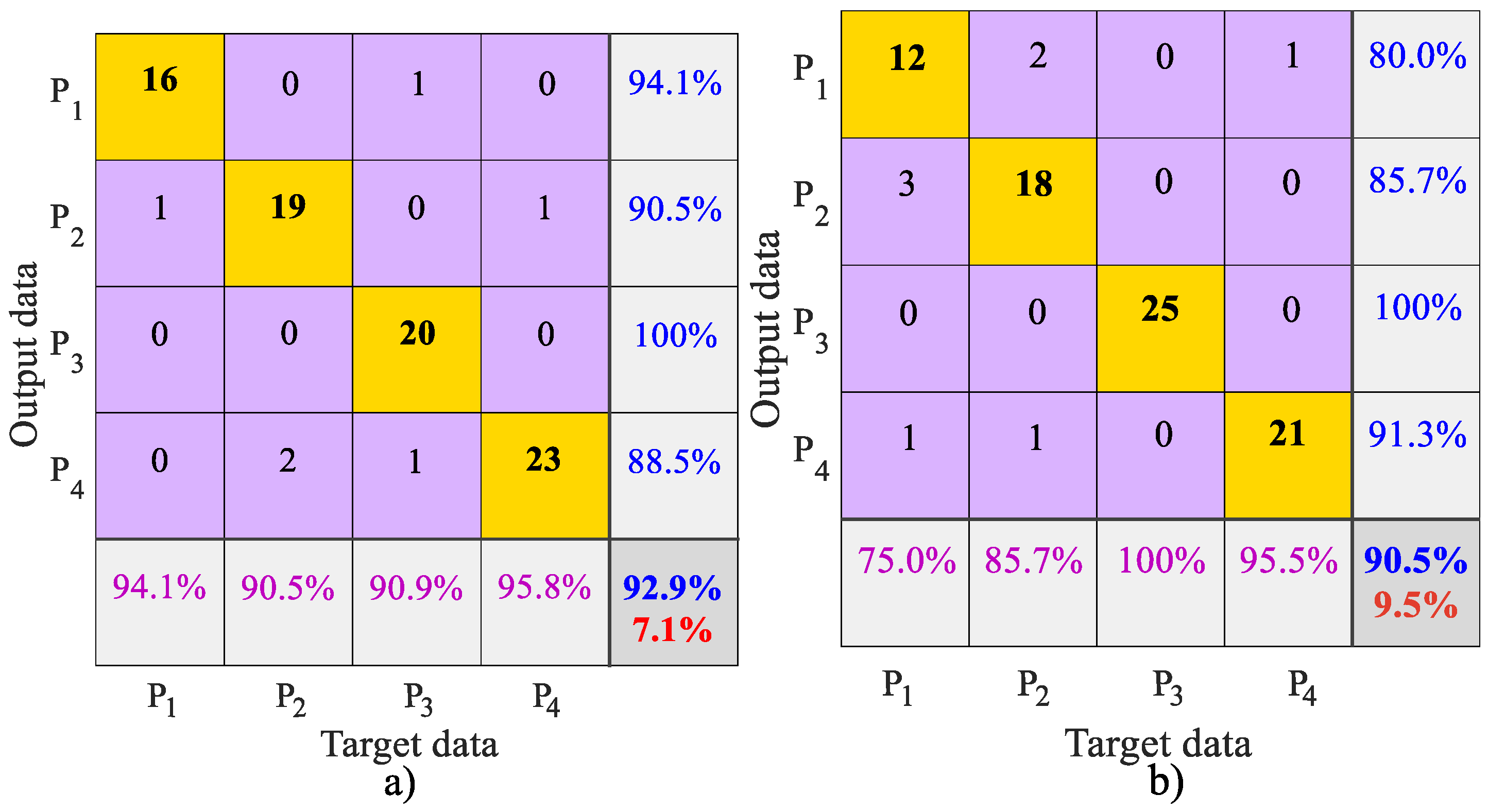
After a series of tests, the results to classify each posture, $P_1$, $P_2$, $P_3$, and $P_4$, are presented and analyzed through confusion matrices, accuracy, and the kappa coefficient for the SVM method. The results based on the confusion matrix are presented in Figure 6; this allows the number of classified images with a concordance agreement to be counted to define data confidence. The best results of the classification are obtained with the characterized images in set $S_1$. These results describe that the postures $P_1$ and $P_3$ achieve the best identification percentages, with 100% and 94.1%, while $P_2$ and $P_4$ obtain 90.5% and 88.5%, respectively. These percentages are achieved by using feature vector $V_1$ in the space color RGB, which are shown in Figure 6a. The classification percentages of feature vector $V_2$ are shown in Figure 6b; the highest accuracy is for $P_3$, with 100%, while the posture $P_4$ is classified with 91.3%. The precision achieved by $P_1$ and $P_2$ is 80% and 85.7%, respectively, with samples of color components in HSV. Therefore, set $V_1$ describes the postures with the best discrimination. The total positive percentage of the classification in $V_1$ is 92.9%, with an error of 7.1%, in comparison with $V_2$ with 90.5%.

Following the same procedure, the confusion matrices were obtained for the classification based on the SVM by using the PCA components. The results are illustrated in Figure 7. Here, the accuracy reached for the sample $V_1$ in the RGB color component is 69%, while, for the sample vector, $V_2$ in the HSV color component is 70.2%. It can be noted that the performance of the SVM based on PCA is lower than that of the SVM with the vectors $V_1$ and $V_2$ previously structured. The accuracy difference to classify the postures based on RGB and HSV color components is 23.9% and 20.3%, respectively.

Regarding the results obtained by the CNNs previously described, the architectures MobileNet and DenseNet121 obtain the best classification results with a total accuracy of 96% and 94%, respectively. The CNNs based on VGG-16 achieve a 92% effectiveness for classifying the postures in bed. The three architectures proposed perfectly identified the position $P_2$ and $P_3$, except for VGG-16, which obtained an accuracy of 80% in $P_3$. Here, the lowest results of CNNs identifying the posture $P_4$ were obtained by VGG-16 with 86.67% and MobileNet with 92.86%. Meanwhile, the posture $P_1$ was identified with different percentages of 90% for the VGG-16, 94.74% for MobileNet, and 86.36% for DenseNet121.

The results of each classification method are summarized in

Table 6. Comparison between the classification of the different feature vectors.

Data	Vector	$\mathit{ACC}$	${\mathit{P}}_1$	${\mathit{P}}_2$	${\mathit{P}}_3$	${\mathit{P}}_4$	kappa
$S_1$	$V_1$	92.9%	94.1%	90.5%	100%	88.5%	0.904
	$V_2$	90.5%	80.0%	85.7%	100%	91.3%	0.871
$S_2$	$V_1$	86.9%	90.5%	95.0%	72.0%	94.4%	0.825
	$V_2$	82.1%	85.0%	81.8%	94.7%	69.6%	0.762
	PCARGB	69.0%	76.9%	66.7%	54.8%	82.1%	0.590
	PCAHSV	70.2%	66.7%	68.4%	57.1%	83.3%	0.596
	CNNVGG-16	92%	90%	100%	80%	86.67%	0.83
	CNNMobileNet	96%	94.74%	100%	100%	92.86%	0.944
	CNNDenseNet121	94%	86.36%	100%	100%	100%	0.9154

, where the accuracy percentages and the kappa values are presented. The worst results based on the kappa metric are obtained by the SVM with PCA method. This method reaches $kappa=0.590$ in the RGB color component and $kappa=0.596$ in the HSV color component. The best accuracy is obtained by the CNNs based on the MobileNet architecture method, with a 96% total accuracy and $kappa=0.944$, followed by the CNNs with DenseNet, which obtain an accuracy of 94% and $kappa=0.9154$. Our proposed approach achieves higher precision and kappa values, slightly outperforming the metrics achieved by the CNN based on VGG-16. These minimal differences are 0.9% in total accuracy and 0.074 for kappa values. Despite our proposal being located in third place according to the results presented in Table 6, the differences concerning the second and first place are 1.1% and 3.1% in total accuracy and 0.0114 and 0.04 in kappa values. It should be noted that CNNs are more complex methods, and are specialized in image classification. However, this comparison was realized to show the grade of precision that can be achieved with a technique that more simply selects the optimal texture descriptors, i.e., the descriptors to achieve the maximal accuracy for the in-bed image classification.

It should be noted that CNNs are more complex, robust, and specialized methods for image classification than an SVM. However, this comparison was conducted to showcase the level of precision that can be achieved with a simpler technique by selecting optimal texture descriptors, i.e., the descriptors for the SVM that yield the highest accuracy for classifying in-bed posture images.

An ROC curve presents the concept of discrimination. The Y-axis of the ROC curve graph represents the proportion of true positives over the total data belonging to one position (sensitivity), and the X-axis represents the proportion of false positives over the total data of another position (specificity). Therefore, an ROC curve plot illustrates the ’proportion of true positives’ (Y-axis) versus the ’proportion of false positives’ (X-axis) for each cut-off point of a classification test whose measurement scale is continuous. A line is drawn from point 0.0 to point 1.1, representing the diagonal or non-discrimination line. This line describes what would be the ROC curve of a classification test unable to discriminate [40], for example, one class 1 ($P_1$) versus class 2 ($P_2$), because each cut-off point that composes it determines the same proportion of true positives and false positives. A discrimination test will have a greater identification capacity to the extent that its cut-off points plot an ROC curve as far as possible from the non-discrimination line, as close as possible to the left and upper sides of the graph.

For a graphic comparison of performance, the ROC curves are plotted in Figure 8; these graphs describe the relationship of $TPR$ against the $FPR$ results that show the scoring classifier [40]. In Figure 8a,b, the posture $P_3$ reaches the coordinate (0, 1), obtaining a perfect classification by using both feature vectors $V_1$ and $V_2$ in RGB and HSV color components, respectively. The postures $P_1$, $P_2$, and $P_4$ are near to the perfect coordinate in Figure 8a, almost closer than the numbers computed employing the feature vector $V_2$ in the HSV space color. In the same way, Figure 9 shows the ROC curve for the SVM and PCA methods. In Figure 9a, a considerable distance from the perfect classification for the postures $P_1$, $P_2$, and $P_3$ can be noted, with an accuracy of 76.9%, 66.7%, and 54.8%, respectively, while the best classification is for the samples for $P_4$ with an accuracy of 82.1%. Figure 9b shows that the scores of the SVM with PCA for the HSV and RGB color components are similar, with accuracy levels of $P_1$, $P_2$, and $P_3$ being 66.7%, 68.4%, and 57.1%, respectively. The ROC curve closest to perfect classification is the one for the posture $P_4$, with 83.3%, in Figure 9b.

In spite of the classification accuracy being less than that reported in [23], it is worth highlighting that the principal purpose of this work was to simplify the stage of image pre-processing. The results obtained employing the proposed methodology are considered excellent based on established metrics. Additionally, it should be considered that the number of patient positions to be identified was increased and that only basic techniques were employed, such as a median filter and histogram equalization.

In the literature, different methodologies have been proposed in which image pre-processing is used for feature extraction and the identification of objects, with different algorithms presenting high accuracy. Additionally, for future researchers, applying the utility of these results and using our proposal in monitoring medical patients with varying characterized parameters would be beneficial. However, some of the processes are robust and complex due to the implementation involving a series of intricate mathematical calculations. One purpose of differentiating between in-bed postures was to demonstrate that such methods can indeed be simple and applicable to other areas.

In this study, some limitations and considerations involve optical devices and experimental issues that affect the quality of the sample image. Environmental and real conditions in hospitals, such as changes in object hue due to luminosity, external objects, textures, camera and sensor distance, and time, can influence image acquisition in patients. Regarding limitations in the image processing area and the time consumed by computing limits, there are two situations. Firstly, the time for image pre-processing and sample conditioning for feature extraction. For this work, the raw images were in low resolution, aligning with the image quality and the proposed feature extraction methodology. Secondly, the time for the training and validation phases used for the classifiers. To select a binary classifier, it is necessary to identify the behavior of the samples through a cross-validation process, depending on the number of samples and the portion of training data to use. The approach of this study was to use selected features of the images as the proposed optimal texture descriptors for in-bed postures. According to the final results, high accuracy performances were obtained with these features; therefore, they are considered useful for future studies applied to medical uses. With these results, some characteristic color components converted into texture descriptors have sufficient class separability.

5. Conclusions

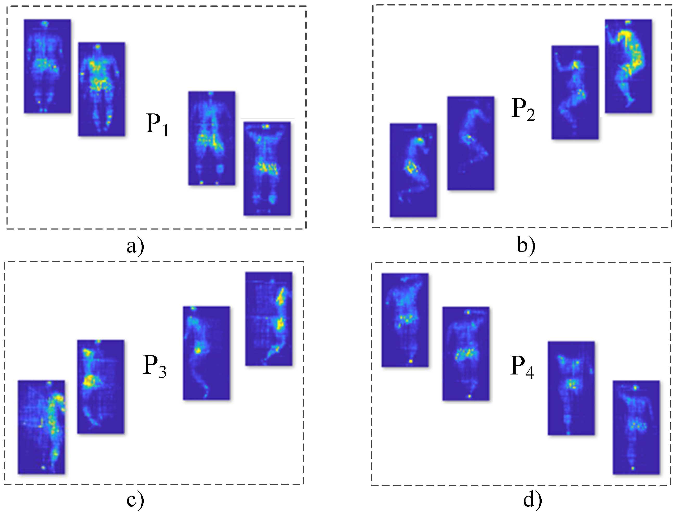
In this work, we proposed the identification of a patient’s posture in bed based on Support Vector Machine training with minimal sample preconditioning. The images were analyzed based on three important stages: sample conditioning, feature extraction, and classification. In the sample conditioning stage, the images are submitted to histogram equalization and a median filter, aiming to avoid complex and computationally heavy pre-processing for the images to be classified. Based on the database description, two experiments were carried out by applying the median filter (MF) to all samples and by using the same filter only for $P_3$ because it presented an external object. From this phase, it was corroborated that the position $P_3$ required an additional treatment due to an obstacle that made it difficult to appreciate the position of the patient. However, it was demonstrated in the first experiment that an MF is enough to remove the disturbances in the images of position $P_3$ and thus improve their classification accuracy. The identification of samples $P_1$, $P_2$, and $P_4$ was affected if the MF was applied; this was corroborated with the accuracy and kappa metrics in a second experiment.

Due to the characteristics of the images depicting patient positions, the selection of texture descriptors was a challenging task. Twenty texture descriptors were employed, and the optimal ones were chosen based on two well-known metrics: ANOVA and the Tukey test. These parameters suggest that different texture descriptors can be utilized based on the color component, whether RGB or HSV.

Nevertheless, in the classification stage, the results suggest that the RGB color component is the most effective for classifying the pressure database of patients. It was also confirmed that the best feature vector can be formed with the data of contrast, correlation, sum of squares, difference of variance, sum average, and information measure of correlation. The classification performance using these variables achieved an accuracy of 92.9% and a kappa of 0.904. Specifically, position $P_3$ could be perfectly classified as long as an MF was applied beforehand. The positions $P_1$, $P_2$, and $P_4$ obtained distinction percentages of 94.1%, 90.5%, and 88.5%, respectively. Despite the widespread use of an SVM with PCA for image classification, this technique showed lower performance, as demonstrated by confusion matrices, kappa values, and ROC curves.

Aiming to assess the performance of our proposal, Convolutional Neural Networks were implemented with different architectures to serve as a reference point. Specifically, CNNs based on MobileNet and DenseNet121 obtained the best results, although with minimal differences of 1.1% and 3.1% in total accuracy and 0.0114 and 0.04 in kappa values, respectively. Therefore, this comparison demonstrates and categorizes the precision that can be achieved by using an SVM while selecting the optimal texture descriptors.

This work proposes simplifying the image pre-processing phase to achieve the classification of a patient’s position in bed by adequately training a Support Vector Machine. The conclusions drawn from this study can assist inexperienced researchers in classifying pressure images and reducing sample preparation time and guide the selection of appropriate color components and texture descriptors.

References

1. Mansfield, S.; Obraczka, K.; Roy, S. Pressure injury prevention: A survey. IEEE Rev. Biomed. Eng. 2019, 13, 352–368. [Google Scholar] [CrossRef]
2. Parish, J.M. Sleep-related problems in common medical conditions. Chest 2009, 135, 563–572. [Google Scholar] [CrossRef] [PubMed]
3. Cenggoro, T.W.; Pardamean, B. A systematic literature review of machine learning application in COVID-19 medical image classification. Procedia Comput. Sci. 2023, 216, 749–756. [Google Scholar]
4. Wilson, A.; Gupta, K.; Koduru, B.H.; Kumar, A.; Jha, A.; Cenkeramaddi, L.R. Recent Advances in Thermal Imaging and its Applications using Machine Learning: A Review. IEEE Sens. J. 2023, 23, 3395–3407. [Google Scholar] [CrossRef]
5. Chandra, M.A.; Bedi, S.S. Survey on SVM and their application in image classification. Int. J. Inf. Technol. 2021, 13, 1–11. [Google Scholar] [CrossRef]
6. Grandini, M.; Bagli, E.; Visani, G. Metrics for Multi-Class Classification: An Overview. arXiv 2020, arXiv:2008.05756. [Google Scholar]
7. Hearst, M.A.; Dumais, S.T.; Osuna, E.; Platt, J.; Scholkopf, B. Support vector machines. IEEE Intell. Syst. Their Appl. 1998, 13, 18–28. [Google Scholar] [CrossRef]
8. Bennett, S.; Ren, Z.; Goubran, R.; Rockwood, K.; Knoefel, F. In-bed mobility monitoring using pressure sensors. IEEE Trans. Instrum. Meas. 2015, 64, 2110–2120. [Google Scholar] [CrossRef]
9. Lee, H.J.; Hwang, S.H.; Lee, S.M.; Lim, Y.G.; Park, K.S. Estimation of body postures on bed using unconstrained ECG measurements. IEEE J. Biomed. Health Inform. 2013, 17, 985–993. [Google Scholar]
10. Barsocchi, P. Position recognition to support bedsores prevention. IEEE J. Biomed. Health Inform. 2012, 17, 53–59. [Google Scholar] [CrossRef]
11. Hittawe, M.M.; Sidibé, D.; Mériaudeau, F. Bag of words representation and SVM classifier for timber knots detection on color images. In Proceedings of the 2015 14th IAPR International Conference on Machine Vision Applications (MVA), Tokyo, Japan, 18–22 May 2015; pp. 287–290. [Google Scholar] [CrossRef]
12. Beya, O.; Hittawe, M.; Sidibé, D.; Mériaudeau, F. Automatic Detection and Tracking of Animal Sperm Cells in Microscopy Images. In Proceedings of the 2015 11th International Conference on Signal Image Technology and Internet Based Systems (SITIS), Bangkok, Thailand, 23–27 November 2015; pp. 155–159. [Google Scholar] [CrossRef]
13. Rivera-romero, C.A.; Palacios-hernández, E.R.; Vite-chávez, O.; Reyes-portillo, I.A. Early-Stage Identification of Powdery Mildew Levels for Cucurbit Plants in Open-Field Conditions Based on Texture Descriptors. Inventions 2024, 9, 8. [Google Scholar] [CrossRef]
14. Rivera-romero, C.A.; Palacios-hernández, E.R.; Trejo-durán, M.; Olivera-reyna, R.; Morales-saldaña, J.A. Visible and near-infrared spectroscopy for detection of powdery mildew in Cucurbita pepo L. leaves. J. Appl. Remote Sens. 2020, 14, 044515. [Google Scholar] [CrossRef]
15. Cruz-Santos, W.; Beltrán-Herrera, A.; Vázquez-Santacruz, E.; Gamboa-Zúñiga, M. Posture classification of lying down human bodies based on pressure sensors array. In Proceedings of the 2014 International Joint Conference on Neural Networks (IJCNN), Beijing, China, 6–11 July 2014; pp. 533–537. [Google Scholar]
16. Dweekat, O.Y.; Lam, S.S.; McGrath, L. Machine Learning Techniques, Applications, and Potential Future Opportunities in Pressure Injuries (Bedsores) Management: A Systematic Review. Int. J. Environ. Res. Public Health 2023, 20, 796. [Google Scholar] [CrossRef]
17. Godoy, D.A.; Carrizosa, J.; Aguilera, S.; Videtta, W.; Jibaja, M.; on behalf of Latin America Brain Injury Consortium (LABIC) Members. Current practices for intracranial pressure and cerebral oxygenation monitoring in severe traumatic brain injury: A Latin American survey. Neurocrit. Care 2023, 38, 171–177. [Google Scholar] [CrossRef]
18. Liu, T.J.; Wang, H.; Christian, M.; Chang, C.W.; Lai, F.; Tai, H.C. Automatic segmentation and measurement of pressure injuries using deep learning models and a LiDAR camera. Sci. Rep. 2023, 13, 680. [Google Scholar] [CrossRef]
19. Clever, H.M.; Grady, P.L.; Turk, G.; Kemp, C.C. Bodypressure-inferring body pose and contact pressure from a depth image. IEEE Trans. Pattern Anal. Mach. Intell. 2022, 45, 137–153. [Google Scholar] [CrossRef]
20. Stern, L.; Roshan Fekr, A. In-Bed Posture Classification Using Deep Neural Network. Sensors 2023, 23, 2430. [Google Scholar] [CrossRef]
21. Silva, A.; Metrôlho, J.; Ribeiro, F.; Fidalgo, F.; Santos, O.; Dionisio, R. A review of intelligent sensor-based systems for pressure ulcer prevention. Computers 2022, 11, 6. [Google Scholar] [CrossRef]
22. Sastry, S.S.; Kumari, T.V.; Rao, C.N.; Mallika, K.; Lakshminarayana, S.; Tiong, H.S. Transition temperatures of thermotropic liquid crystals from the local binary gray level cooccurrence matrix. Adv. Condens. Matter Phys. 2012, 2012, 527065. [Google Scholar] [CrossRef]
23. Hajari, N.; Lastre-Dominguez, C.; Ho, C.; Ibarra-Manzano, O.; Cheng, I. Longitudinal In-Bed Pressure Signals Decomposition and Gradients Analysis for Pressure Injury Monitoring. Sensors 2021, 21, 4356. [Google Scholar] [CrossRef]
24. Grimm, R.; Sukkau, J.; Hornegger, J.; Greiner, G. Automatic patient pose estimation using pressure sensing mattresses. In Bildverarbeitung für die Medizin 2011: Algorithmen-Systeme-Anwendungen Proceedings des Workshops vom 20.-22. März 2011 in Lübeck; Springer: Berlin/Heidelberg, Germany, 2011; pp. 409–413. [Google Scholar]
25. Zhu, H.; Liang, H.; Xiao, F.; Wang, G.; Hussain, R. Pressure Image Recognition of Lying Positions Based on Multi-Feature Value Regularized Extreme Learning Algorithm. Appl. Math. Nonlinear Sci. 2022, 8, 559–572. [Google Scholar] [CrossRef]
26. Liu, S.; Yin, Y.; Ostadabbas, S. In-bed pose estimation: Deep learning with shallow dataset. IEEE J. Transl. Eng. Health Med. 2019, 7, 1–12. [Google Scholar] [CrossRef]
27. Xiao, J. SVM and KNN ensemble learning for traffic incident detection. Phys. A Stat. Mech. Its Appl. 2019, 517, 29–35. [Google Scholar] [CrossRef]
28. Zhang, S. Cost-Sensitive KNN Classification. Neurocomputing 2019, 391, 234–242. [Google Scholar] [CrossRef]
29. Haralick, R.M.; Shanmugam, K.; Dinstein, I.H. Textural features for image classification. IEEE Trans. Syst. Man Cybern. 1973, 3, 610–621. [Google Scholar] [CrossRef]
30. Lilliefors, H.W. On the Kolmogorov-Smirnov test for normality with mean and variance unknown. J. Am. Stat. Assoc. 1967, 62, 399–402. [Google Scholar] [CrossRef]
31. Fisher, R.A. Studies in crop variation. I. An examination of the yield of dressed grain from Broadbalk. J. Agric. Sci. 1921, 11, 107–135. [Google Scholar] [CrossRef]
32. Neter, J.; Kutner, M.H.; Nachtsheim, C.J.; Wasserman, W. Applied Linear Statistical Models; Irwin: Chicago, IL, USA, 1996. [Google Scholar]
33. Deng, X.; Liu, Q.; Deng, Y.; Mahadevan, S. An improved method to construct basic probability assignment based on the confusion matrix for classification problem. Inf. Sci. 2016, 340–341, 250–261. [Google Scholar] [CrossRef]
34. Salla, R.; Wilhelmiina, H.; Sari, K.; Mikaela, M.; Pekka, M.; Jaakko, M. Evaluation of the confusion matrix method in the validation of an automated system for measuring feeding behaviour of cattle. Behav. Process. 2018, 148, 56–62. [Google Scholar] [CrossRef]
35. Ma, J.; Du, K.; Zheng, F.; Zhang, L.; Gong, Z.; Sun, Z. A recognition method for cucumber diseases using leaf symptom images based on deep convolutional neural network. Comput. Electron. Agric. 2018, 154, 18–24. [Google Scholar] [CrossRef]
36. Griffel, L.; Delparte, D.; Edwards, J. Using Support Vector Machines classification to differentiate spectral signatures of potato plants infected with Potato Virus Y. Comput. Electron. Agric. 2018, 153, 318–324. [Google Scholar] [CrossRef]
37. Rumpf, T.; Mahlein, A.K.; Steiner, U.; Oerke, E.C.; Dehne, H.W.; Plümer, L. Early detection and classification of plant diseases with Support Vector Machines based on hyperspectral reflectance. Comput. Electron. Agric. 2010, 74, 91–99. [Google Scholar] [CrossRef]
38. Ohsaki, M.; Wang, P.; Matsuda, K.; Katagiri, S.; Watanabe, H.; Ralescu, A. Confusion-Matrix-Based Kernel Logistic Regression for Imbalanced Data Classification. IEEE Trans. Knowl. Data Eng. 2017, 29, 1806–1819. [Google Scholar] [CrossRef]
39. Vieira, S.M.; Kaymak, U.; Sousa, J.M.C. Cohen’s kappa coefficient as a performance measure for feature selection. In Proceedings of the International Conference on Fuzzy Systems, Barcelona, Spain, 18–23 July 2010; pp. 1–8. [Google Scholar]
40. Jiang, Y. Receiver Operating Characteristic (ROC) Analysis of Image Search-and-Localize Tasks. Acad. Radiol. 2020, 27, 1742–1750. [Google Scholar] [CrossRef] [PubMed]
41. Pouyan, M.B.; Birjandtalab, J.; Heydarzadeh, M.; Nourani, M.; Ostadabbas, S. A pressure map dataset for posture and subject analytics. In Proceedings of the 2017 IEEE EMBS International Conference on Biomedical & Health Informatics (BHI), Orlando, FL, USA, 16–19 February 2017; pp. 65–68. [Google Scholar]
42. Goldberger, A.L.; Amaral, L.A.N.; Glass, L.; Hausdorff, J.M.; Ivanov, P.C.; Mark, R.G.; Mietus, J.E.; Moody, G.B.; Peng, C.K.; Stanley, H.E. PhysioBank, PhysioToolkit, and PhysioNet: Components of a New Research Resource for Complex Physiologic Signals. Circulation 2000, 101, e215–e220. [Google Scholar] [CrossRef]
43. Richard, A.; Johnson, D.W.W. Applied Multivariate Statistical Analysis, 6th ed.; Pearson, Prentice Hall: Hoboken, NJ, USA, 2007. [Google Scholar]
44. Hoaglin, D.C. John W. Tukey and Data Analysis. Stat. Sci. 2003, 18, 311–318. [Google Scholar] [CrossRef]
45. Bagheri, M.A.; Montazer, G.A.; Kabir, E. A subspace approach to error correcting output codes. Pattern Recognit. Lett. 2013, 34, 176–184. [Google Scholar] [CrossRef]
46. Bagheri, M.A.; Gao, Q.; Escalera, S. A genetic-based subspace analysis method for improving Error-Correcting Output Coding. Pattern Recognit. 2013, 46, 2830–2839. [Google Scholar] [CrossRef]
47. Krizhevsky, A.; Sutskever, I.; Hinton, G.E. Imagenet classification with deep convolutional neural networks. In Proceedings of the Advances in Neural Information Processing Systems 25: 26th Annual Conference on Neural Information Processing Systems 2012, Lake Tahoe, NV, USA, 3–6 December 2012. [Google Scholar]
48. Rasheed, J. Analyzing the Effect of Filtering and Feature-Extraction Techniques in a Machine Learning Model for Identification of Infectious Disease Using Radiography Imaging. Symmetry 2022, 14, 1398. [Google Scholar] [CrossRef]
49. Attallah, O.; Ragab, D.A. Auto-MyIn: Automatic diagnosis of myocardial infarction via multiple GLCMs, CNNs, and SVMs. Biomed. Signal Process. Control 2023, 80, 104273. [Google Scholar] [CrossRef]
50. Wei, Y.; Liu, Y.; Song, H.; Lu, Z. A Method of Rainfall Detection from X-band Marine Radar Image Based on the Principal Component Feature Extracted. IEEE Geosci. Remote. Sens. Lett. 2023, 20, 3501105. [Google Scholar] [CrossRef]
51. LeCun, Y.; Bottou, L.; Bengio, Y.; Haffner, P. Gradient-based learning applied to document recognition. Proc. IEEE 1998, 86, 2278–2324. [Google Scholar] [CrossRef]
Figure 1. Postures of patients are considered for the identification of the pressure position: (a) dorsal decubitus, (b) lateral decubitus, (c) lateral decubitus with an external object, and (d) dorsal decubitus with crossed legs.
Bdcc 08 00013 g001
Figure 2. Methodology for patient posture identification.
Bdcc 08 00013 g002
Figure 3. ANOVA of the features: (a) mean values of CPROMS, (b) mean values of DVARHG. The red plus sign (+) in both figures indicates the outliers.
Bdcc 08 00013 g003
Figure 4. Features maps: (a) feature CONTRH versus SAVGHB of P 1 and P 4 ; and (b) feature CORRMR versus DVARHG of P 3 and P 4 .
Bdcc 08 00013 g004
Figure 5. Training data in 2D and 3D hyperplanes, circles and asterisks are the class data of position P1 and P2, respectively. (a) features SOSVHS and IDMNCV for data in P 1 , (b) features SOSVHS and IDMNCV for data in P 2 , and (c) 2D hyperplane for both classes.
Bdcc 08 00013 g005
Figure 6. Confusion matrices obtained for the multiple classifications for characterized images in set S 1 : (a) classified data in V 1 samples in color components of RGB, and (b) classified data in V 2 samples in color components of HSV.
Bdcc 08 00013 g006
Figure 7. Confusion matrices obtained for the multiple classifications: (a) classified data with PCA components in V 1 samples in color components of RGB, and (b) classified data with PCA components in V 2 samples in color components of HSV.
Bdcc 08 00013 g007
Figure 8. ROC curves obtained for the multiple classifications: (a) classified data in V 1 samples in color components of RGB, and (b) classified data in V 2 samples in color components of HSV.
Bdcc 08 00013 g008
Figure 9. ROC curves obtained for the multiple classifications: (a) classified data with PCA components in V R G B samples in color components of RGB, and (b) classified data with PCA components in V H S V samples in color components of HSV.
Bdcc 08 00013 g009