Data-Driven Fracture Morphology Prognosis from High Pressured Modified Proppants Based on Stochastic-Adam-RMSprop Optimizers; tf.NNR Study

Abstract

Data-driven models with some evolutionary optimization algorithms, such as particle swarm optimization (PSO) and ant colony optimization (ACO) for hydraulic fracturing of shale reservoirs, have in recent times been validated as one of the best-performing machine learning algorithms. Log data from well-logging tools and physics-driven models is difficult to collate and model to enhance decision-making processes. The study sought to train, test, and validate synthetic data emanating from CMG’s numerically propped fracture morphology modeling to support and enhance productive hydrocarbon production and recovery. This data-driven numerical model was investigated for efficient hydraulic-induced fracturing by using machine learning, gradient descent, and adaptive optimizers. While satiating research curiosities, the online predictive analysis was conducted using the Google TensorFlow tool with the Tensor Processing Unit (TPU), focusing on linear and non-linear neural network regressions. A multi-structured dense layer with 1000, 100, and 1 neurons was compiled with mean absolute error (MAE) as loss functions and evaluation metrics concentrating on stochastic gradient descent (SGD), Adam, and RMSprop optimizers at a learning rate of 0.01. However, the emerging algorithm with the best overall optimization process was found to be Adam, whose error margin was 101.22 and whose accuracy was 80.24% for the entire set of 2000 synthetic data it trained and tested. Based on fracture conductivity, the data indicates that there was a higher chance of hydrocarbon production recovery using this method.

1. Introduction

Hydrocarbon production decline [1,2] poses substantive threats to energy sustainability; hence, the demand for resolving this challenge in both conventional and unconventional wells is on a marathon course. Our contemporary research community has enhanced the practical and technical hydraulic fracturing [3,4] means to intensify the recovery of oil and gas in unconventional reservoirs. This well stimulation [5,6] method could also be termed as fracking [7], which consists of passing high-pressure fluids that are simply made of chemical additives, sand, and water (proppants) for opening and holding up channels for the production of excess stored hydrocarbons. However, under this technique, it is often linear to investigate and initiate the fracturing process, observe the fluid flow from the fractured formation, and determine the fracture propagation. The primary purpose of hydraulic fracturing is to increase the hydrocarbon productive index targeted at low-permeable formations, for instance, shale formations [8,9,10]. Hydrocarbon production decline is mostly attributed to formation damage, which is one of the reasons emanating from poorly designed drilling and completion fluids [11,12]. The leak of these fluids seals off the formation of pore throats and void spaces [13,14], preventing the flow of fluids from the formation to the wellbores.

Empirically, it is often prudent to study and design appropriate hydraulic fracturing methods before their inception. Researchers [15,16] have investigated several ways to stimulate non-productive wells coupled with effective predictive analysis by designing numerical models to counter poor flow regimes in the formation. Successful predictive studies are the result of the type and geometric structure of the formation morphology, the type of proppants [17,18], and their mechanical stress capabilities, fracture length, and infinite conductivity.

Based on physics-driven models, Suri-Islam-Hossain (SIH) [19] used an extended finite element method (XFEM) to simulate fluid leak-off effects under proppant transport for fracture propagation. Their hydrodynamic integrated model, as shown in Figure 1, demonstrated an XFEM initial pressure for fracturing set to 7497 psi. The results of their study indicate that the proppants’ transport and their relative suspension are largely influenced by an increased rate of injection.

However, subsequent physics-driven simulations [20], conducted by Wang et al. [21], explain how permeability testing for coal bed methane deposits can be carried out safely and effectively without blow-ups. The authors further indicated that the direction of fracture can become uncertain, since fracture channels tend to expand in the direction of principal stress. In Figure 2, Wang et al., using PFC2D, modeled and simulated a directional hydraulic fracturing (DHF), whose findings demonstrated that fracture propagation can be regulated using the DHF approach [22], as this overcomes its original or principal stress, and for this reason, it is asserted that fracture propagation extends along and perpendicular to the slotting.

Martyushev et al. [23] expounded the use of machine learning (ML) for the predictive optimization of reservoir pressure in directional hydraulic fracturing (DHF) carbonate reservoirs. Their study considered hydraulically fractured Well 423 on the D₃fm oil deposit site, as presented in Figure 3. The focus of ML modeling was based simply on the interactions and influences of the neighboring wells (9070, 430, 424, 427, 433) on Well 423, before and after DHF. The relationship for the model was referred to as the coefficient of correlation (r), as demonstrated in Figure 3. The result of their research indicates that the higher the correlation coefficient, the more accurate the reservoir pressure prediction, and as demonstrated, Well 423, before and after DHF, presents increased pressure levels, indicating a red region, and low reservoir pressures correspond to a lower correlation coefficient, indicating a yellow and blue region.

However, reservoir pressures migrating from neighboring wells 429, 427, and 424 to Well 423 before DHF present a case where the tendency of a well blowout is obvious while drilling. The ML predictive analysis presented in the case of Martyushev et al. [23] supports managerial decision-making to optimize drilling operations.

Nonetheless, there has also been abundant research on data-driven models for the prediction of hydraulic fracturing well stimulation. Dong et al. [24] optimized fracture parameters using data-driven algorithms. The authors explain that there is a high cost and driven uncertainty associated with fracture spacing and half-length. For this reason, the research expounded on the use of an evolutionary optimization algorithm (EOA) for parametric fracture optimization. Hence, their resulting numerical simulation, based on a gradient-boosted decision tree, random forest, support-vector machine, and multilayer perception (MLP), demonstrated in Figure 4, shows that among all the four production-prediction models, one of the EOA, i.e., particle swarm optimization (PSO), produced the highest net present value.

In recent times and in this current study, the neural network prognosis architectures have not only looked at the deep neural network Keras architectures, such as sequential, functional, and subclassing API analysis, but there has also been an advance investigation on the use of convolutional neural networks (CNN) and recurrent neural networks (LSTM), with a proposed extension of optimizers. However, the likes of Elbaz and Shen [25,26,27] have proven in their research the possibility of advancing the neural network architecture prognosis.

In other words, while maintaining the TensorFlow Keras Sequential API architecture, a synthetic dataset for training and testing using the most effective neural network optimizers from the current study is essential for reducing predicted errors in the petroleum fracking sector. The stochastic gradient descent [28,29] algorithm used is evaluated for big datasets, with the intention of selecting batches at random from the total dataset for each iteration. In order to roughly obtain a minimum, this optimizer sorts to shuffle the data at random for each iteration. Most importantly, in the case of gradient descent, it is not suitable for large datasets, as the convex algorithm does not randomly shuffle the entire dataset, but instead, for every iteration, the whole data is focused on finding the approximate minimum. For this reason, SGD produces a lot of noise, based on the batches for each iteration, and to reach the desired approximate minimum, a higher number of iterations is needed, which brings the total time for computation to a record high. However, it is purported that SGD with higher iterations can optimize noise cancellation. Nonetheless, another means of countering noise production is by the extension of SGD with momentum, imagine propping a naturally fractured and low permeable formation, where the momentum of the proppants in the natural fracture formation gains maximum convergence. Most of all, while considering the momentum, the likelihood that the desired minimum could be reached is high; hence, careful regulation of the number of iterations is needed for better optimization.

Adaptive moment estimation (Adam) [30] is an extension of SGD [31]; whereas, the weights of the entire network under training are optimized by a single learning rate, Adam, on the other hand, concentrates on upgrading each network’s weights. Based on its wide usage, several researchers have indicated it as the benchmark for deep learning and standard optimization approaches, since it does not support overtime computation and requires less memory for computation, thereby reducing the entire cost of computation. While there has been overwhelming research curiosity for better adaptation of deep learning optimizers, previous studies in the research community [32,33], few intelligent applications based on the root mean square propagation (RMSprop) optimizer have been published. This adaptive optimizer takes its roots from RProp, known as resilient backpropagation. Since RProp contradicts the theory behind stochastic gradient descent, RMSprop was developed as an extension of RProp. As a result, just as Adam focuses on each network’s weight, so does RMSprop. In this case, a weight’s specified learning rate is gradually split by the size of its most recent gradients, averaged over time, and determined using the mean square method. Figure 5 presents an illustrative performance of the current study’s choice of gradient and adaptive optimizers for the manipulation and tweaking of the synthetic fracking dataset to optimize the predictive petroleum industry. The previous neural network modeling, as conducted by [34], defined an input shape of 28, 28, 1 and upon successfully splitting the improvised data at a dtype float 32, built its model using Keras Sequential, and with activation functions set to ReLU, and SoftMax introduced a loss function of cross entropy under the following optimizers, seen in Figure 5. It is empirically significant to note that the resulting experiment indicates that the Adam optimizer achieved the best performing algorithm, as it is followed by RMSprop and SGD.

Another typical study on various optimizers based on different datasets conducted by Mohapatra et al. [35] demonstrates the efficacy of AdaSwarm compared to SGD, AdaGrad, AdaDelta, RMSprop, AMSGrad, Adam, emulating SGD with PSO parameters. The adaptive gradient-based optimizers under a series of compiled models were used for deep learning comparative mean squared and mean absolute errors (MSE/MAE) loss function analysis. The authors, while focusing on swarm intelligence, thus AdaSwarm and the exponentially weighted momentum particle swarm optimizer (EMPSO), whose various parameters were measured against gradient descent (GD), defined the capabilities of these optimizers to execute precise gradient approximations, which further exposes the novelty of their conducted research. Based on the neural network algorithms (EMPSO/AdaSwarm) and subsequent differential and non-differential models proposed by Mohapatra et al. [35], it resulted that the gradient-free adaptive swarm intelligence algorithm (AdaSwarm) had proven superior over other optimizers, such as RMSprop, SGD, and Adam.

In this current study, stochastic gradient descent (SGD), and Adam and RMSprop optimizers for hydrocarbon production recovery predictive analysis were modeled based on high-pressure hydraulic fracturing. Moreover, the concentration of gradient descent and adaptive optimizers is used to train and test hydraulic fracturing on numerically modeled datasets, based on the Google TensorFlow machine learning algorithms. A linear and non-linear neural network regression (NNR) based on these selected optimizers was used to optimize highly modified proppants [36] for effective fracture propagation and production recovery.

2. Methods

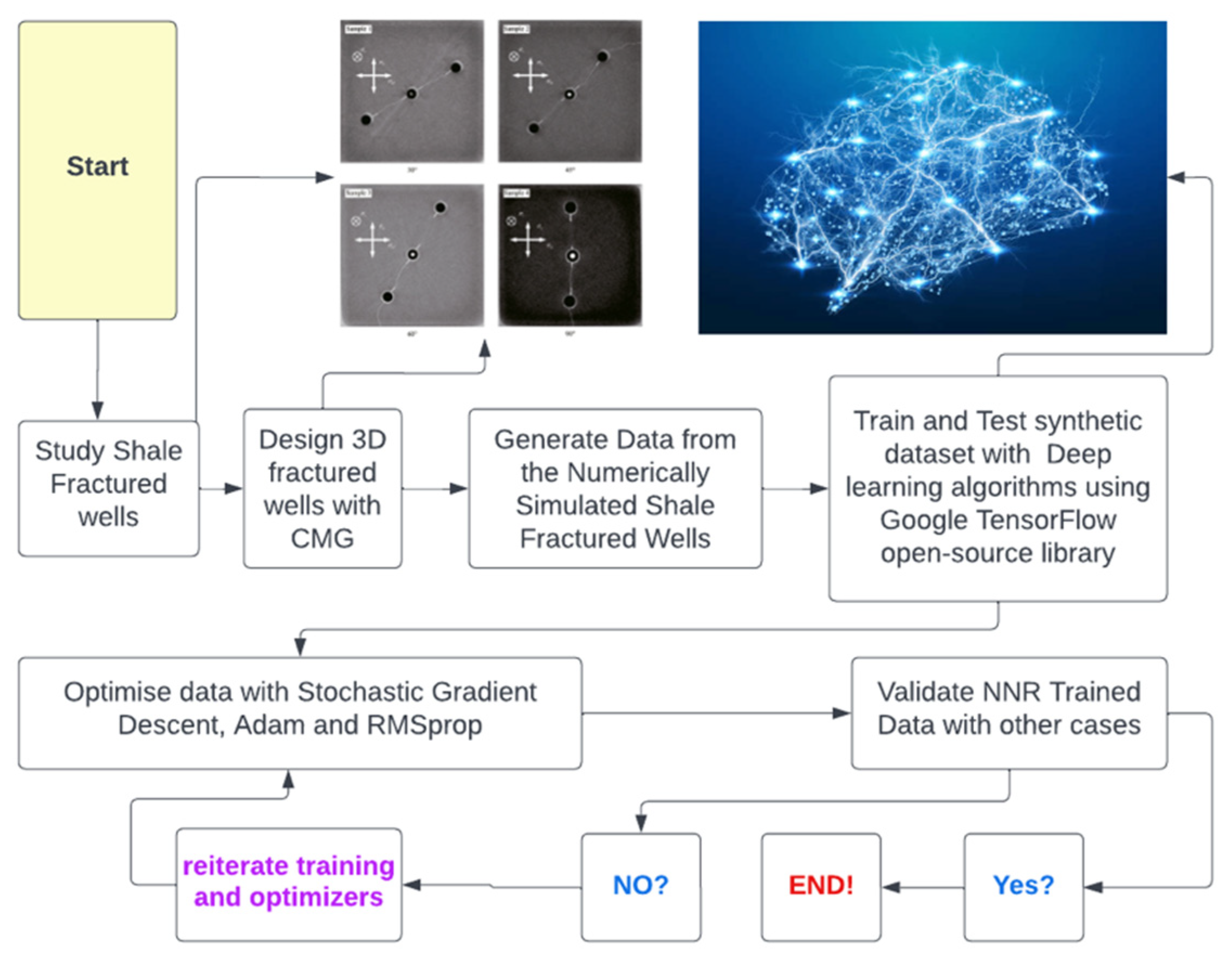
2.1. Data-Driven Modeling

Building up models generates data that emanates from intelligent tools. Being aware of the difficulty in reading log data, it is practical to use synthetic data for modeling, making a clear-cut validation with real data. However, in the absence of physics-driven simulations, as demonstrated in Figure 1, data-driven model analysis can be the easiest computationally intelligent tool at hand. Moreover, the wholistic parameters involved in modeling data generation originate from the initial reservoir conditions, hydraulic fracture characteristics, and hydrocarbon production. Figure 6 provides the detailed methods and flow chart for an effective propped fracture prognosis.

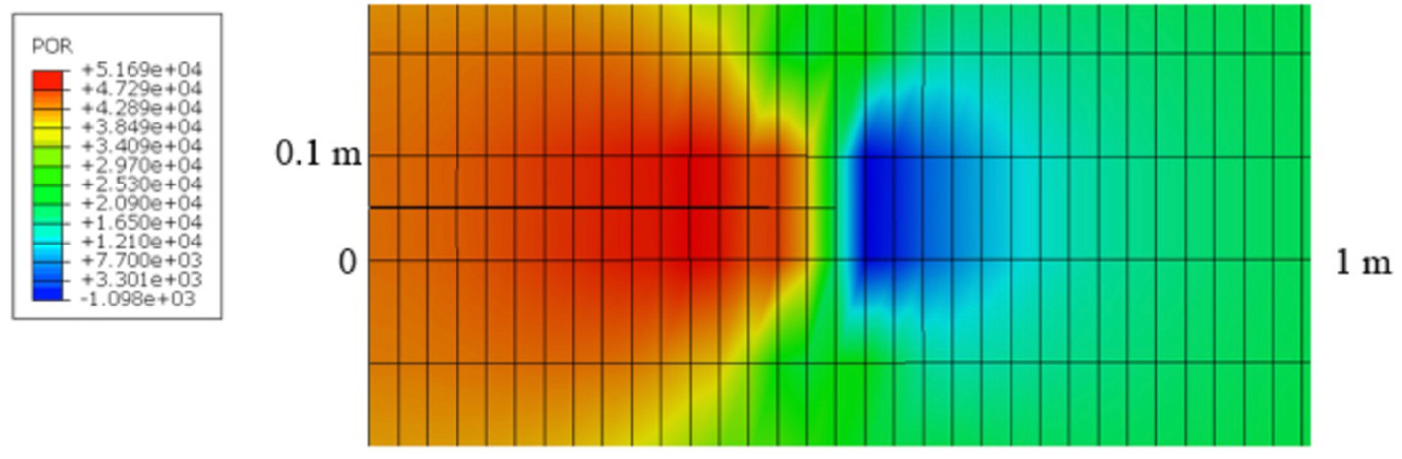
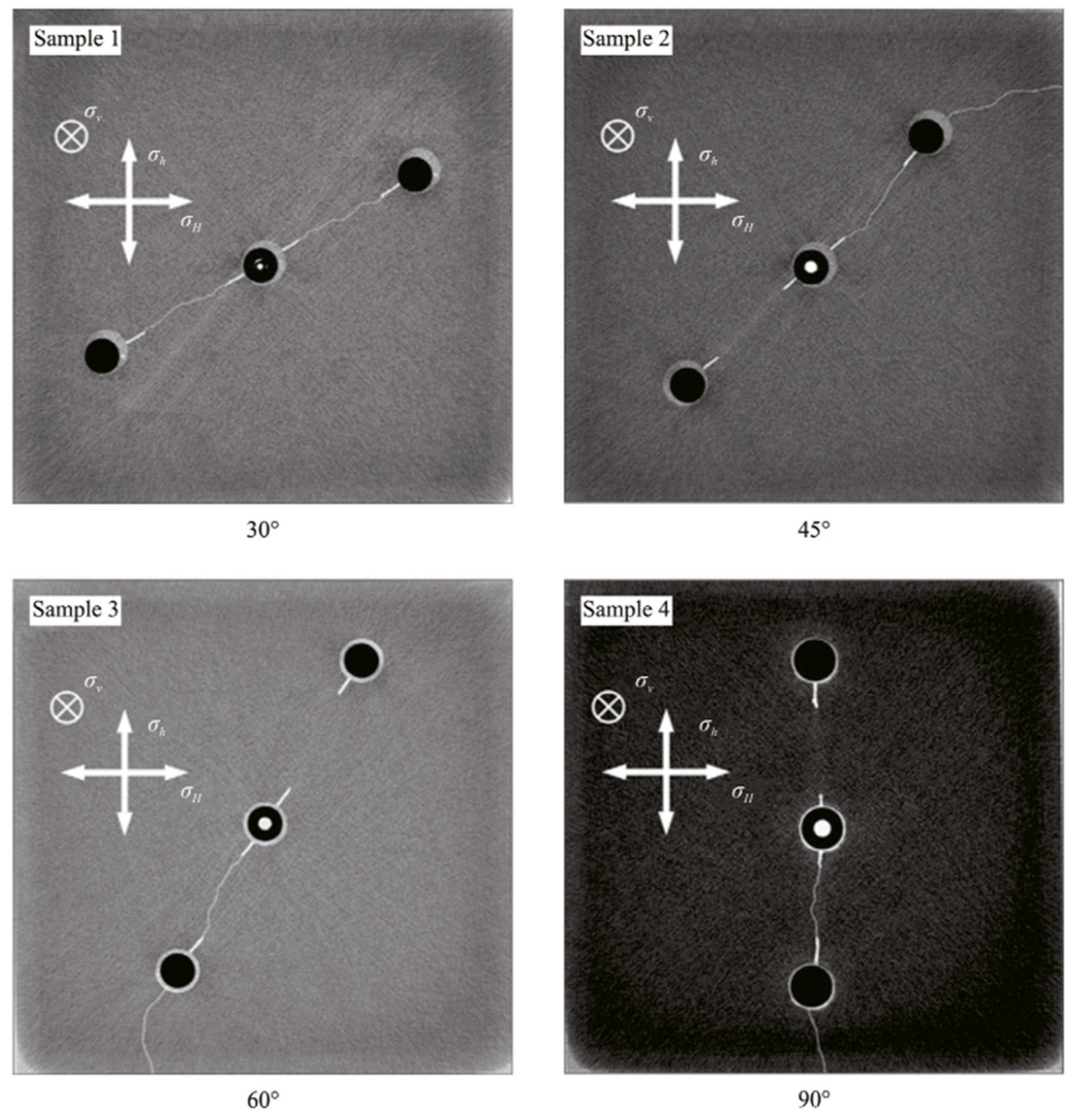
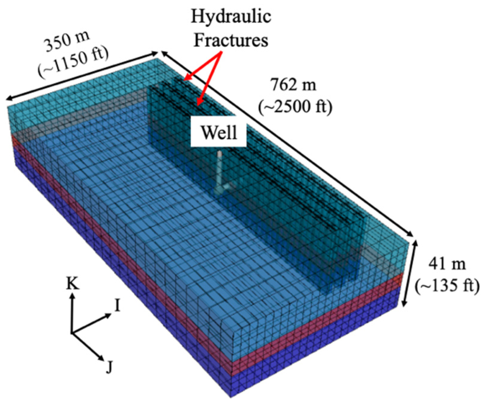
2.2. Numerical Modeling

Based on a commercial black oil simulator, CMG’s integrated third-party geomechanics-based hydraulic fracturing tools, shown in Figure 7, were used to numerically model the data, which generated input and output parameters, with concentrations on porosity ($\mathsf{\varphi }$), height (h), fracture length (L_f), fracture width (w_f), fracture permeability, and a productivity index (flowing bottom-hole pressure, P_wf).

The 2000-dataset model was numerically focused on shale formations. The current study’s 3D design [37,38,39] two-phase flow simulation in assumed vertical reservoirs was saturated with oil and gas. The striated vertical and transverse propped fracture propagation of the simulated reservoir obtained its operation perpendicular to its minimum principal stress, yet in the direction of its maximum principal stress. According to Oritz et al. [40] their study initiated the most appreciable dual-permeability procedure for modeling two-phased shale plays and natural fractures [41]. Their applicable method for simulating naturally induced fractures and hydraulic fractures was made possible by CMG-IMEX. Notwithstanding, input parameters modeled with CMG by Kulga et al. [42] yielded promising hydraulic fracturing [43] parameters for numerically synthesizing the data in

Table 1. Input Parameters for CMG Numerical Modeling.

	Reservoir Conditions				Hydraulic Fracture Parameters						FBHP
	Pi [psi]	T [°F]	Yg	A [acres]	h [ft]	k [md]	ϕ [%]	Lf [ft]	kf [md]	wf [in]	Pwf
Min.	500	100	0.5	1000	60	0.00001	4	500	2000	0.01	510
Max.	5000	300	0.9	2000	500	0.1	30	1500	100000	0.4	756

.

Figure 7. CMG hydraulic fracturing simulation in shale reservoir adapted with permission from Ref. [40], 2021, Arias Ortiz, D. A.

Figure 7. CMG hydraulic fracturing simulation in shale reservoir adapted with permission from Ref. [40], 2021, Arias Ortiz, D. A.

According to the minimum and maximum synthetic data generated, the initiation of propping fractures in vertical shale reservoirs is mostly termed to have initial reservoir conditions with pressures (P_i) of about 500 psi, thermal conditions of 100 degrees Fahrenheit (T), and an area (A) of about 1000 acres. Additionally, while considering an efficient predictive analysis, synthetic data for hydraulic fractures obtained a maximum fracture length (L_f) of 1500 ft at a height (h) of 500 ft and 30% porosity (ϕ) and a fractured permeability (k_f) at 0.1 mD. Nonetheless, the width of the fracture based on the data was from 0.1 to 0.4 to conductively expound the pore channels for higher productivity or to increase flowing bottom-hole pressure.

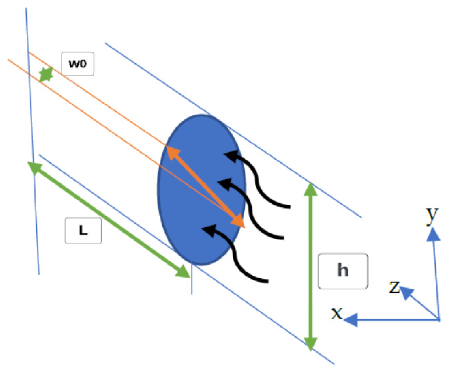
2.3. Fluid-Fracture Equations

Figure 8 schematically demonstrates a one-wing infinite homogenous two-dimensional formation hydraulic fracturing model that was originally proposed by Perkins and Kern, also known literally as the P-K equation [44]. This fracture flow diagram depicts how high-pressure proppants or fluids move in the direction of the x-axis with a constant height of h on the y-axis. The diameter of the fracture morphology on the z-axis remains the width. It is interesting to note that the fracture length is exponentially greater than that of a constant height and width. These are mathematically represented based on the following P-K assumptions:

(a)

There is no storage effect nor fluid leak off.

(b)

At the tip, the net pressure remains zero.

(c)

Fluids are Newtonian and incompressible.

(d)

Fluid injection is assumed to be in constant volumetric flow rate.

(e)

Because much less energy is needed to propagate a fracture than to simply allow the fluid to flow along it, the toughness of the formation can be disregarded.

Young Modulus [45] (vertical plane), E′;

$${\mathrm{E}}^{\prime }=\frac{2\sqrt{{\mathrm{H}}^2-4{\mathrm{y}}^2}}{\mathrm{w}}\mathrm{P},$$

(1)

Young Modulus (plane strain), E′;

$${\mathrm{E}}^{\prime }=\frac{\mathrm{E}}{1-{\mathrm{v}}^2},$$

(2)

Maximum fracture width, w_m;

$${\mathrm{W}}_{\mathrm{m}}=\frac{2\mathrm{H}}{{\mathrm{E}}^{\prime }}\mathrm{P},$$

(3)

Fluid continuity [46,47];

$$\frac{\partial \mathrm{q}}{\partial \mathrm{x}}+\mathrm{q}\mathrm{L}+\frac{\partial \mathrm{A}}{\partial \mathrm{t}}=0,$$

(4)

The continuity based on the assumption (a) would be further expressed as;

$$\frac{\partial \mathrm{q}}{\partial \mathrm{x}}=0,$$

(5)

Integrating the Newtonian laminar fluid where Equation (3) is at x = 0;

$${\mathrm{w}}_0=0.38{\left(\frac{{\mathrm{Q}}_0\mathsf{\mu }\mathrm{L}}{{\mathrm{E}}^{\prime }}\right)}^{\frac{1}{4}},$$

(6)

Since one of the P-K assumptions [48] is made on a constant flow rate along the fractured axis, attention is given to the fracture length (L), maximum fracture width at the bottom-hole (${\mathrm{w}}_0$), and net pressure at downhole (${\mathrm{P}}_0$), which are represented as;

$$\mathrm{L}={\left(\frac{625}{409{6\mathsf{\pi }}^3}\right)}^{\frac{1}{5}}{\left(\frac{{{\mathrm{Q}}_0}^3{\mathrm{E}}^{\prime }}{\mathsf{\mu }{\mathrm{H}}^4}\right)}^{\frac{1}{5}}{\mathrm{t}}^{\frac{4}{5}},$$

(7)

$${\mathrm{w}}_0={\left(\frac{640}{{\mathsf{\pi }}^2}\right)}^{\frac{1}{5}}{\left(\frac{{{\mathrm{Q}}_0}^2\mathsf{\mu }}{{\mathrm{E}}^{\prime }\mathrm{H}}\right)}^{\frac{1}{5}}{\mathrm{t}}^{\frac{1}{5}},$$

(8)

$${\mathrm{P}}_0={\left(\frac{80}{{\mathsf{\pi }}^2}\right)}^{\frac{1}{4}}{\times {\left(\frac{1}{4}\right)}^{\frac{1}{5}}\left(\frac{{{{{\mathrm{E}}^{\prime }}^4\mathrm{Q}}_0}^2\mathsf{\mu }}{{\mathrm{H}}^6}\right)}^{\frac{1}{5}}{\mathrm{t}}^{\frac{1}{5}},$$

(9)

Nordgren’s improved model adds storage and leak-off effects to make P-K’s equation more convincing and practical, as presented in Equations (10)–(12) [49,50];

$$\mathrm{L}=\frac{{\mathrm{Q}}_0}{2\mathsf{\pi }{\mathrm{C}}_{\mathrm{L}}\mathrm{H}}{\mathrm{t}}^{\frac{1}{2}}$$

(10)

$${\mathrm{w}}_0=4{\left(\frac{{{\mathrm{Q}}_0}^2\mathsf{\mu }}{{\mathsf{\pi }}^3{\mathrm{E}}^{\prime }{\mathrm{C}}_{\mathrm{L}}\mathrm{H}}\right)}^{\frac{1}{4}}{\mathrm{t}}^{\frac{1}{8}}$$

(11)

$${\mathrm{P}}_0=2{\left(\frac{{{{{\mathrm{E}}^{\prime }}^3\mathrm{Q}}_0}^2\mathsf{\mu }}{{\mathsf{\pi }}^3{\mathrm{C}}_{\mathrm{L}}{\mathrm{H}}^6}\right)}^{\frac{1}{4}}{\mathrm{t}}^{\frac{1}{8}}$$

(12)

For hydrocarbon production recovery in vertical shale wells, there is an inflow of the two-phase process.

Further Fracture Assumptions

• The rate of flow is assumed.
• Fracture is conducted in vertical wells.
• Time for injection is considered.
• Existing proppants at high pressure are included.

2.4. TensorFlow

TensorFlow is an all-inclusive open-source machine learning platform. Its large, versatile ecosystem of tools, libraries, and community resources enables academics to improve the state-of-the-art of machine learning while simultaneously enabling developers to swiftly construct and deploy ML-powered products. TensorFlow was developed by engineers and researchers on the Google Brain team, a division of Google’s Machine Intelligence Research department, for the purpose of conducting machine learning and deep neural network research. The technique is versatile enough to be applied in several other industries. TensorFlow offers non-guaranteed backward compatibility for various languages, in addition to established Python and C++ APIs.

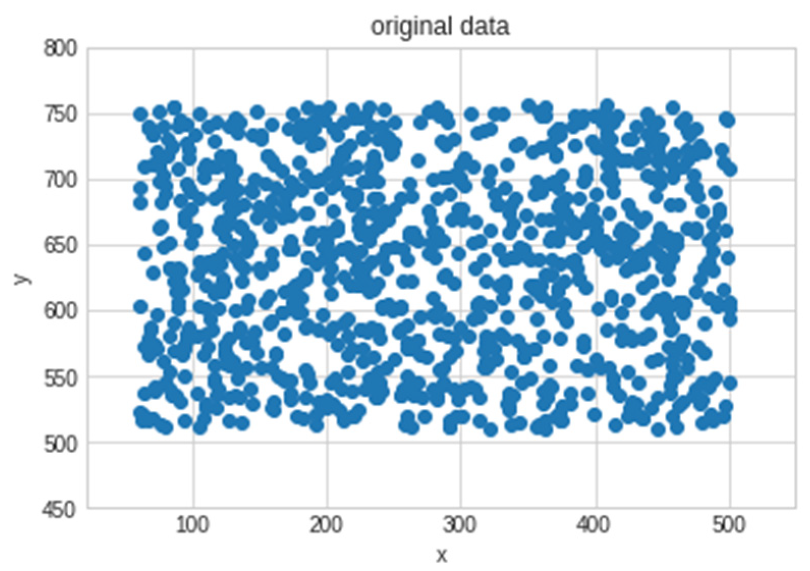
2.4.1. Data Pre-Processing and Splitting

In spite of this, the deep neural network analysis developed for the present study used a linear and non-linear method while focusing on selected optimizers (SGD, Adam, and RMSprop) under the impact of learning rates, activation, and loss functions.

Moreover, there was no need to pre-process or normalize the data because it had already been cleaned before importing, based on the Pandas library. The complete length of the 2000 synthetic data was trained at 80% and tested at 20%.

2.4.2. Deep Neural Network (Non-Linear Regression)

The study generated a model for non-linear regression [51,52,53] to determine the influence and prediction of various fractured input parameters over the production recovery with Keras sequential stable input dense layer of 100, 10 and an output layer shape of 1, shown in Figure 9 and

Table 2. Output screen; standard model summary for all training.

Model: “Proppant_Fracturing_ML_Modeling”
Layer (Type)	Output Shape	Param #
Input_layer (Dense) dense_6 (Dense) output_layer (Dense)	(None, 1000) (None, 100) (None, 1)	2000 100100 101
Total params: 102,201 Trainable params: 102,201 Non-trainable params: 0

. Moreover, while maintaining a learning rate of about 0.01, the activation function for the input layer was set to a rectified linear unit (ReLU; thus, a non-linear activation function intended for deep neural networks).

The generated model for training the data was compiled, setting the loss function to the mean absolute error and the optimizers to the stochastic descent gradient (SGD), Adam, and RMSprop, respectively, for each of the models’ build-ups. Figure 10, Figure 11, Figure 12, Figure 13, Figure 14 and Figure 15 demonstrates loss curves for various input parameters emanating from fractured height, width, length, permeability, and porosity of the formation and fractured conductivity raw synthetic data, validated in Figure 9.

2.4.3. Neural Network (Linear Regression)

Production recovery prediction analysis engaged a linear neural network regressor utilizing the Keras sequential model for the synthetic data. The model was compiled with an input shape of 1 and a linear activation, unlike ReLU, as indicated for the non-linear regressor mentioned earlier. However, while the study maintained its reliability, the model was compiled with the same loss functions (MAE) and selected optimizers for training the model with a 0.01 learning rate and an epoch of 100. Figure 16, Figure 17, Figure 18, Figure 19 and Figure 20 illustrate the predictive version of the linear regression.

3. Results and Discussion

The performances of optimizers for the various regressors used to predict hydraulic fracturing and production recovery are compiled in

Table 3. Keras optimizers for production recovery prediction.

Parameters			Loss Functions/MAE
			h [ft]	ϕ [%]	Lf [ft]	wf [in]	k [md]	Conductivity [mD.in]	Average
Non-Linear	Keras Optimizers	SGD	61.50	399.11	366.46	620.66	61.50	61.72	261.83
		ADAM	125.86	65.46	155.50	93.45	72.6	94.42	101.22
		RMSprop	231.91	106.36	174.33	124.99	169.38	177.10	163.87
Parameters			Loss functions/MAE
			h [ft]	ϕ [%]	Lf [ft]	wf [in]	k [md]	Conductivity [mD.in]	Average
Linear	Keras Optimizers	SGD	347.88	225.58	487.19	255.78	260.98	198.30	295.95
		ADAM	221.07	234.23	157.91	251.87	255.49	134.83	209.23
		RMSprop	220.25	225.56	253.81	249.91	253.81	192.46	232.63

. For better lay understanding, the average of all optimizers based on the various input parameters was obtained. However, Stochastic descent, Adam, and RMSprop optimizers indicated very good performance optimizers, just as other known optimizers demonstrated the capabilities of molding and shaping the fitted model into an accurate form.

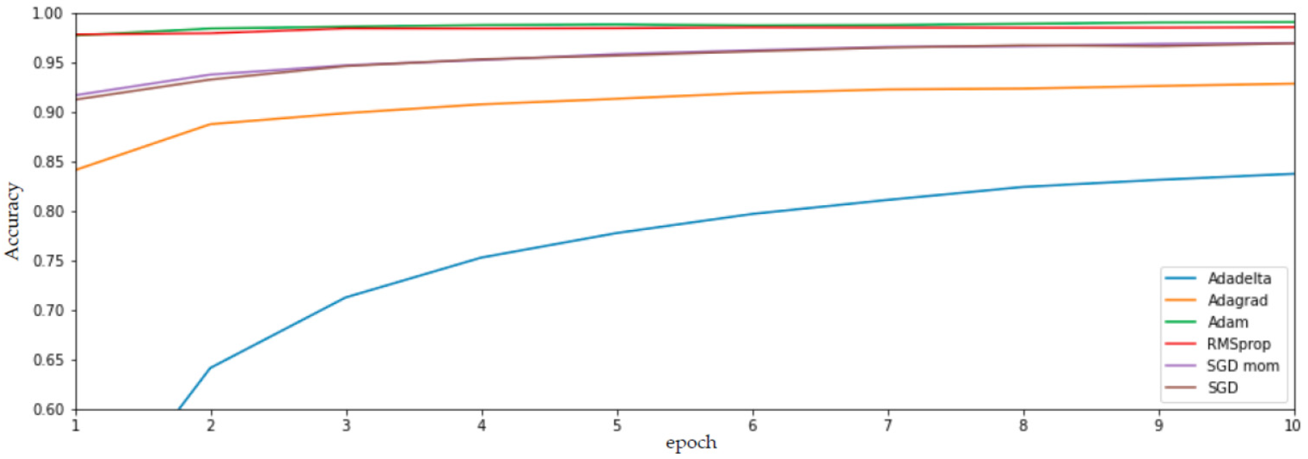
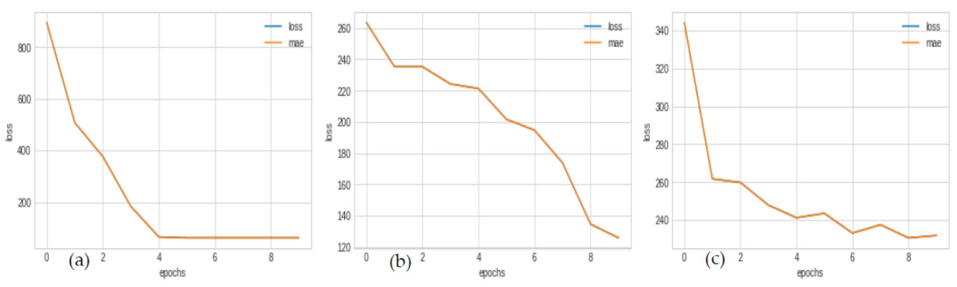
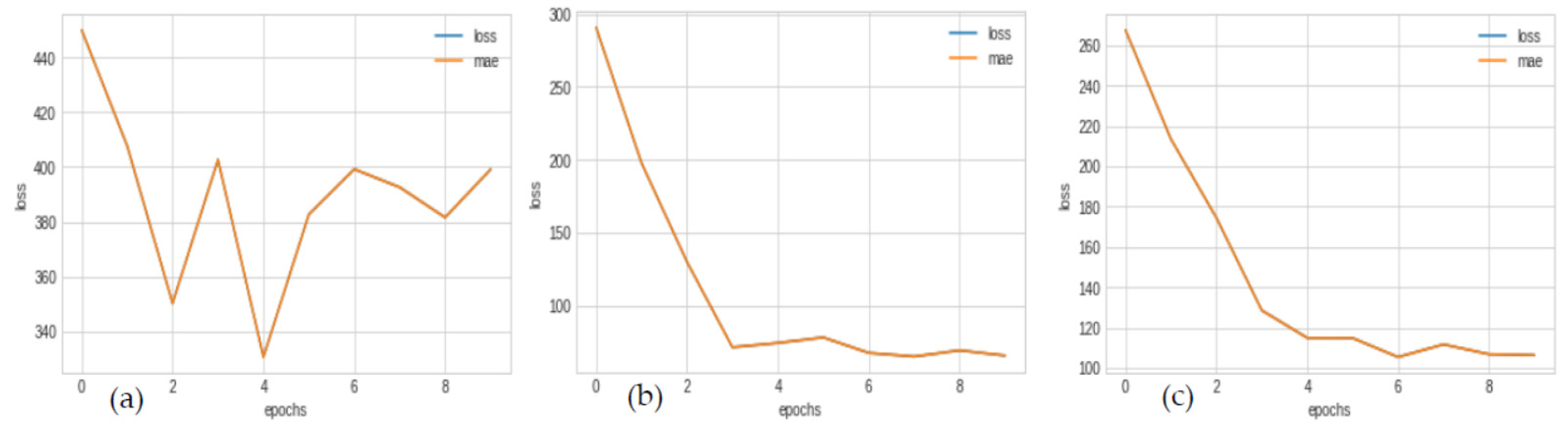
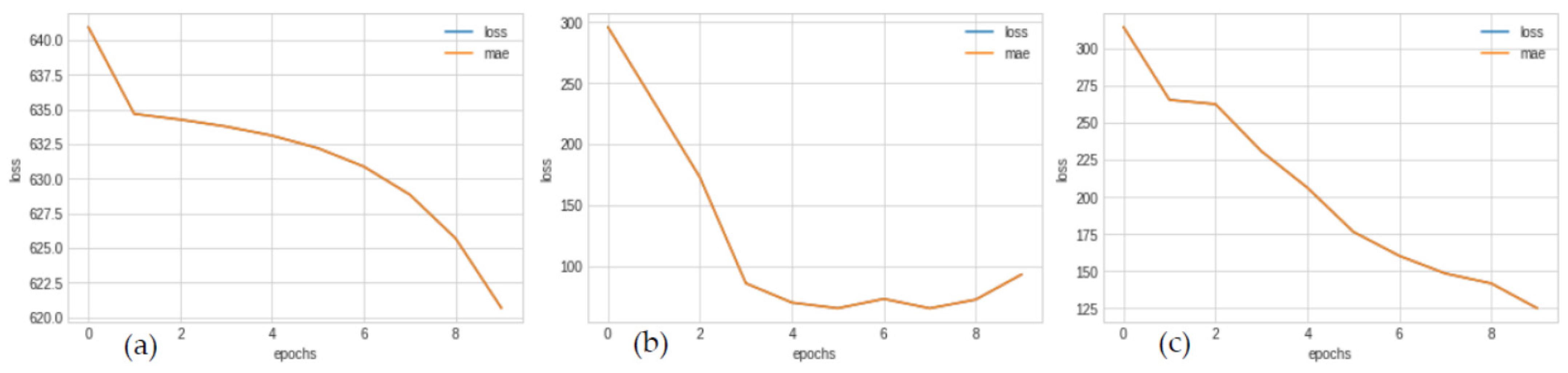
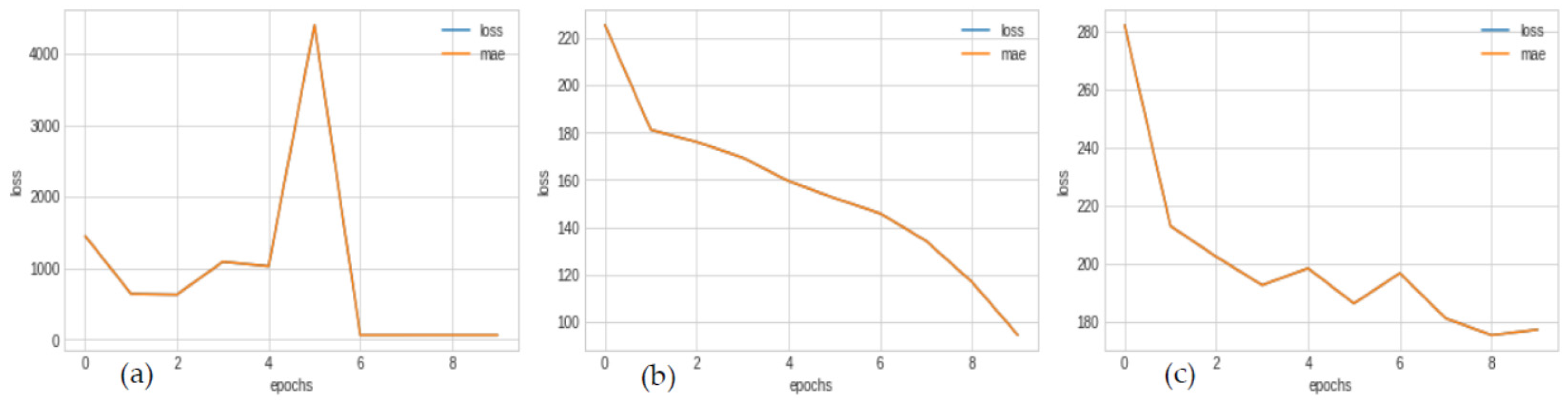
3.1. Non-Linear Optimizers

The performances of Keras optimizers based on the neural network ReLU compiled the model into a non-linear form. The input data parameters, while considering SGD, obtained an average loss function or a mean absolute error of 261.83, Adam’s optimizer computed as 101.22, and RMSprop was 163.87. The final loss comparative analysis indicates that the lower the loss, the more accurate the prediction would be.

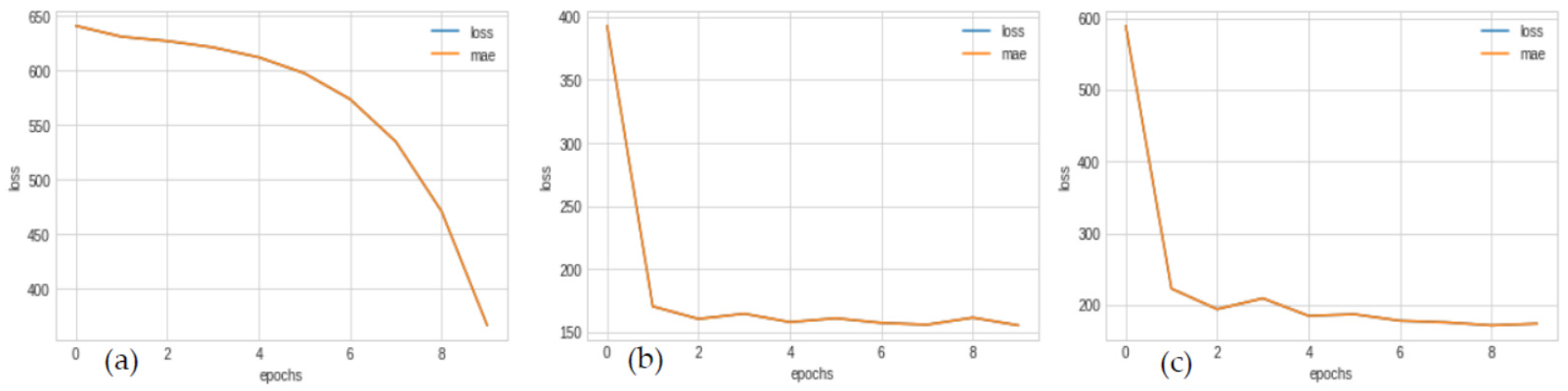
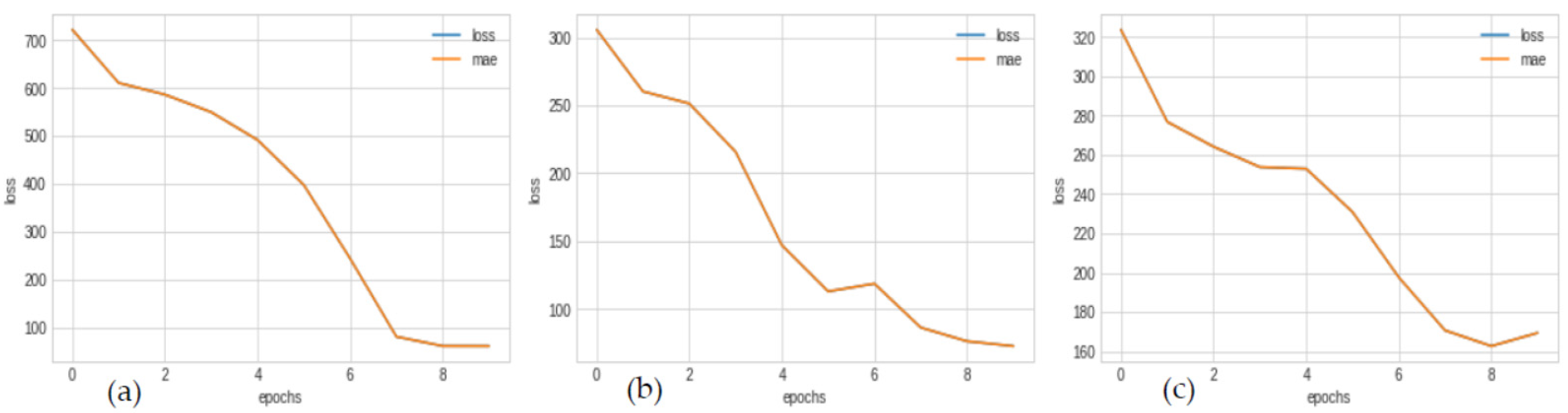
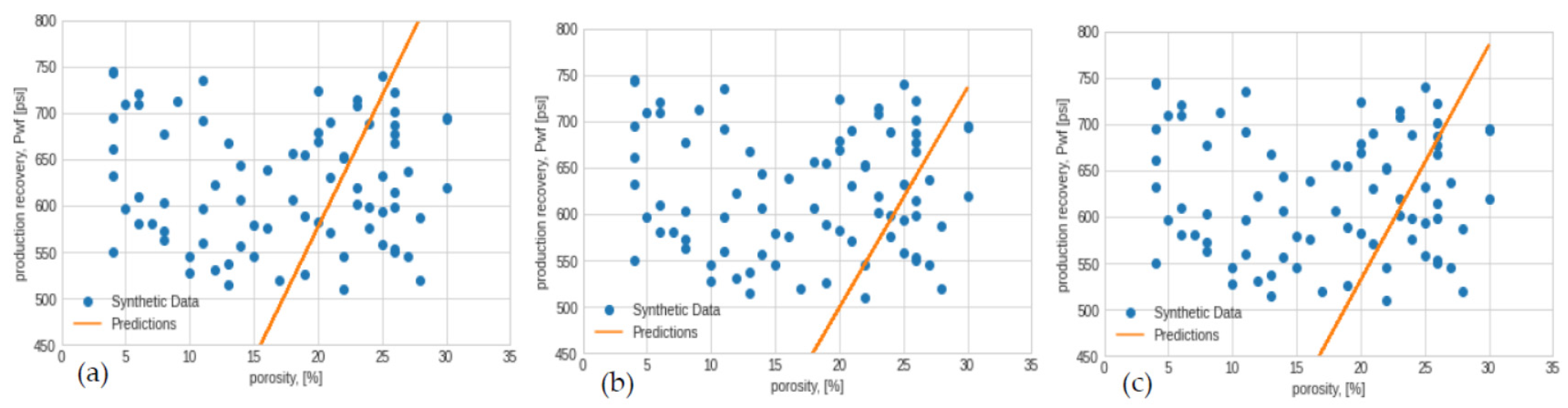
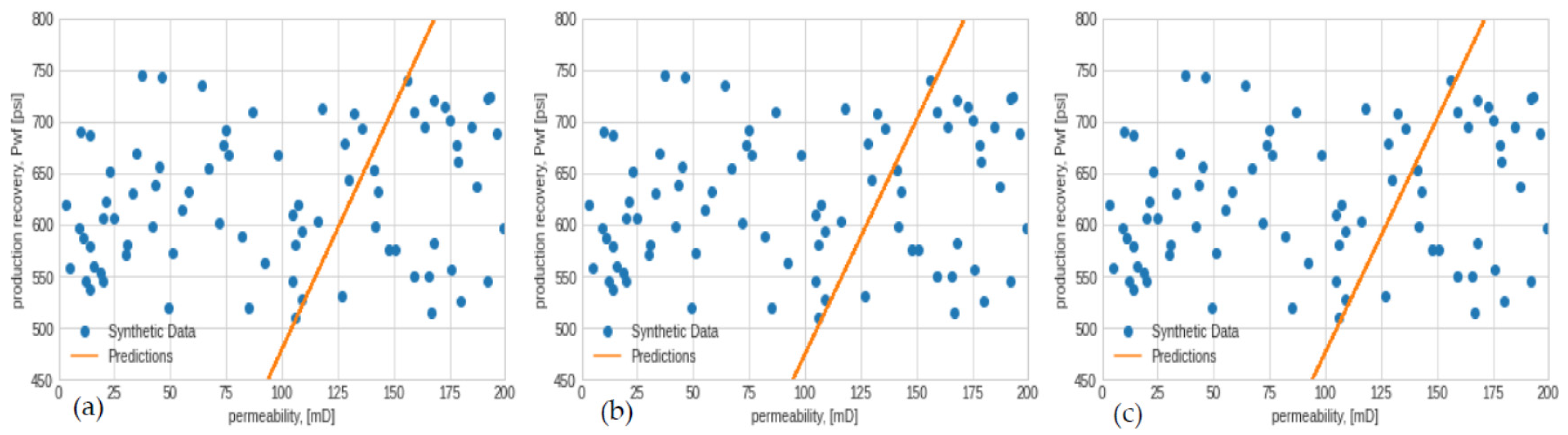
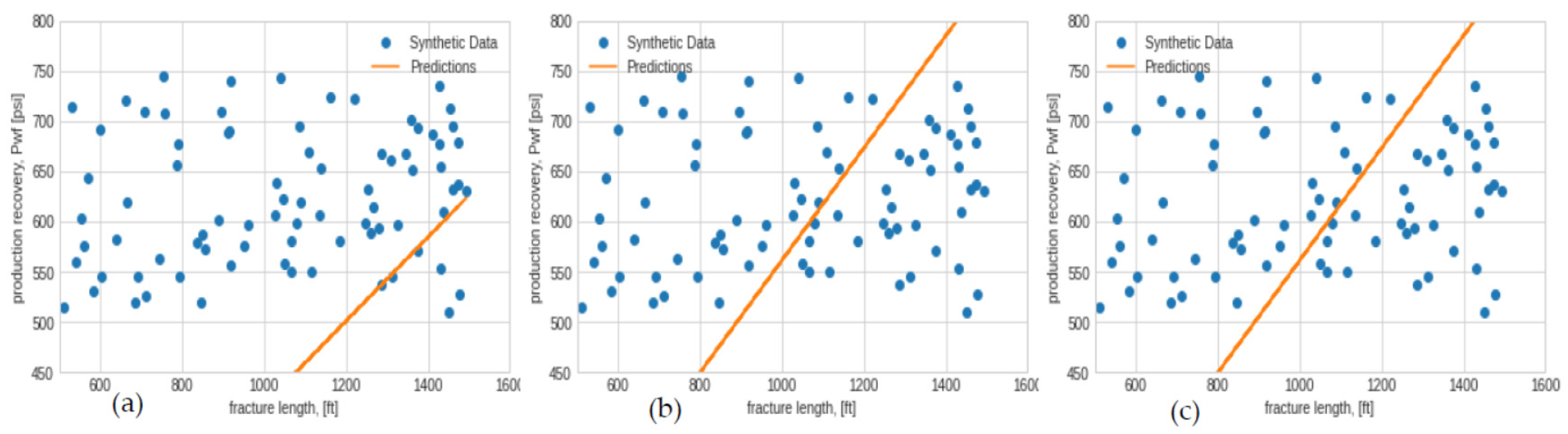
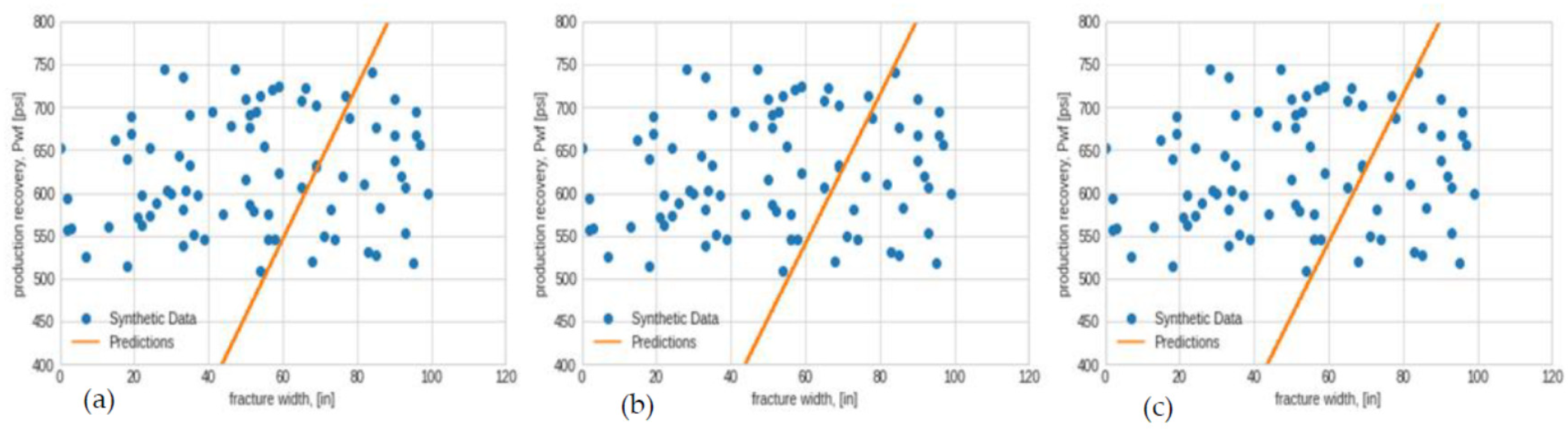
3.2. Linear Optimizers

The model was compiled based on the linear activation function, and the input parameters fitted the models to obtain an average Adam optimizer loss function of 209.23. Generally, the linear optimizers for the fracture propagation data were determined to have performed inadequately, in contrast to the same optimizers for non-linear functions. This could be as a result of inadequate neurons used, unfavorable learning rates, and a limited number of iterations. However, Figure 21. draws out the entire computation for this study, demonstrating the best optimizer. As mentioned earlier, the lower the loss, the higher the performance; hence, from the visual bar graph, Adam demonstrated the lowest loss for the synthetic fracture propagation data.

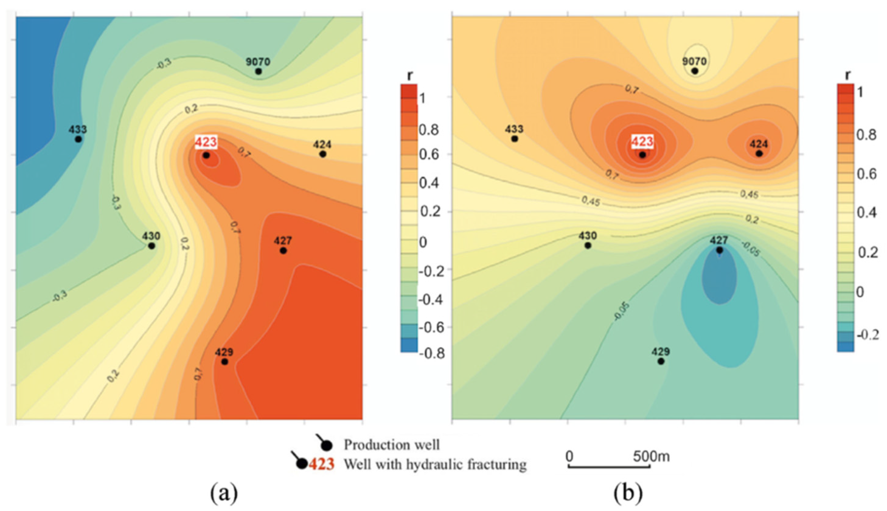
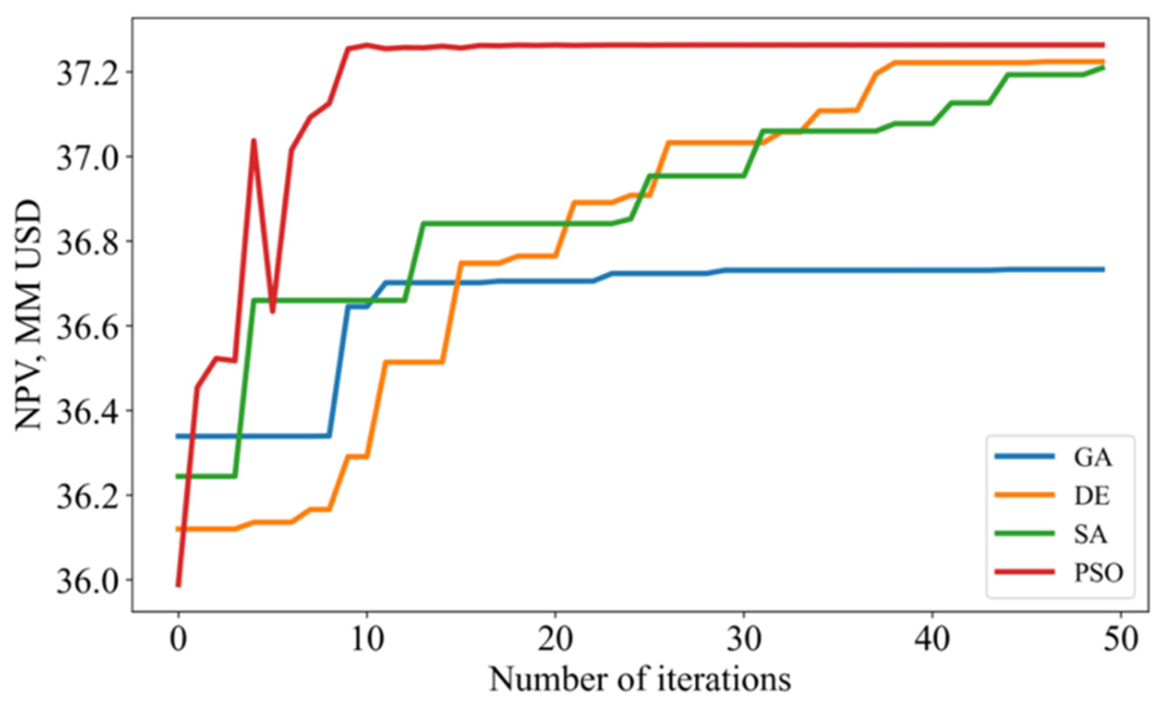
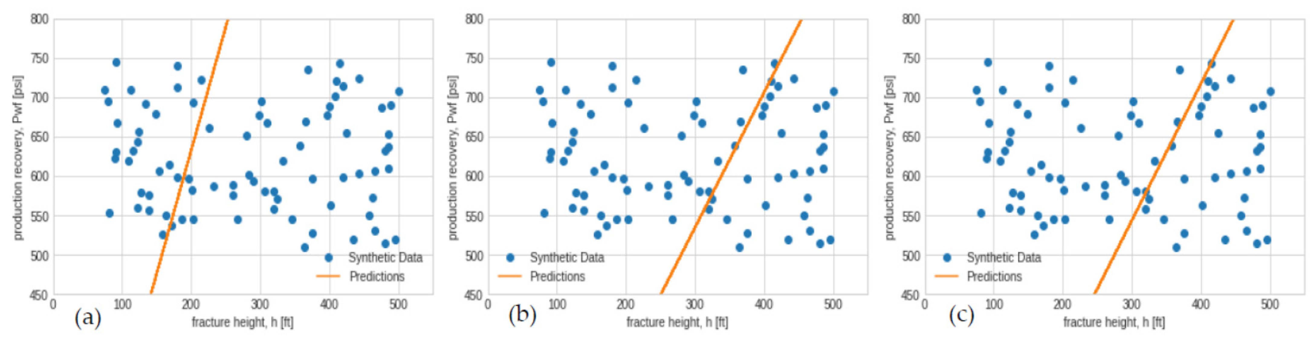
3.3. Production Recovery Optimization

The synthetic data emanating from CMG modeling was shuffled and indexed to read production recovery, as demonstrated in Figure 21. However, the model used for the earlier prediction indicated that, out of the entire 2000 synthetic datasets replicated, the Adam optimizer prediction, with a 101.22 loss function, was at best 80.24% accurate. Production recovery was based on the flowing bottom-hole pressure; hence, a plot to determine the fracture conductivity where the propped fracture tends to convey formation fluids into the wellbore is demonstrated in Figure 22.

The measure of permeability and fracture width from the data generated explains that the shale formation under review has a better chance of maximizing hydrocarbon production.

3.4. Validation and Limitations

The weight of this study was compared with the work of Dong et al. [24], who in recent times developed a machine learning algorithm coupled with other multilayer perception algorithms with an emphasis on particle swarm optimization (PSO). After several tweaks, the authors noticed the PSO, provided the best results, as indicated in Figure 3. Drawing an intense analysis between PSO and Adam optimizers, the current study did not model using PSO, which is recommended for consideration in subsequent research while considering AdaSwarm [25], which is embedded in the NumPy and TensorFlow libraries.

Neural network optimizers, as researched by Mohapatra et al. [25], explicitly provide a comparative analysis of various optimizers, which throws enough light on the current study. In addition, while considering the efficacy of SGD, Adam, and RMSprop, it is quite fair to validate their performances with other relevant datasets. Furthermore, since some of Mohapatra et al.’s derived models consisted of second-order differential equations, validation of their optimizers is best for the current study’s non-linear neural network regressions. In so doing, it is worth noting that, when the average of the previous study’s loss functions from SGD, Adam, and RMSprop withholding tolerance was duly compared, Adam still performed much better, even considering other datasets.

However, it is advisable to keep in mind that there was probably not enough model and other hyperparameter tweaking to enhance optimization. In the case of Adam, the algorithm was able to achieve an accuracy of 80.24%. Most importantly, Adam’s remaining accuracy of 20% could be further optimized to 100% accuracy if long periods of iterations at an epoch of, i.e., 500 to 1000 for both linear and non-linear neural network training could be considered, with a decreasing learning rate of 0.001.

4. Conclusions

The data-driven sensitive machine learning algorithms, with an emphasis on SGD, Adam, and RMSprop optimizers, have indeed paved an additional artificially intelligent way to optimize synthetic data and its input parameters for fracturing hydrocarbon wells with low permeability indexes, and their tendency to optimize production recovery predictions. Moreover, based on high-pressure proppants, the novelty of the study was able to identify, using Google TensorFlow libraries, that:

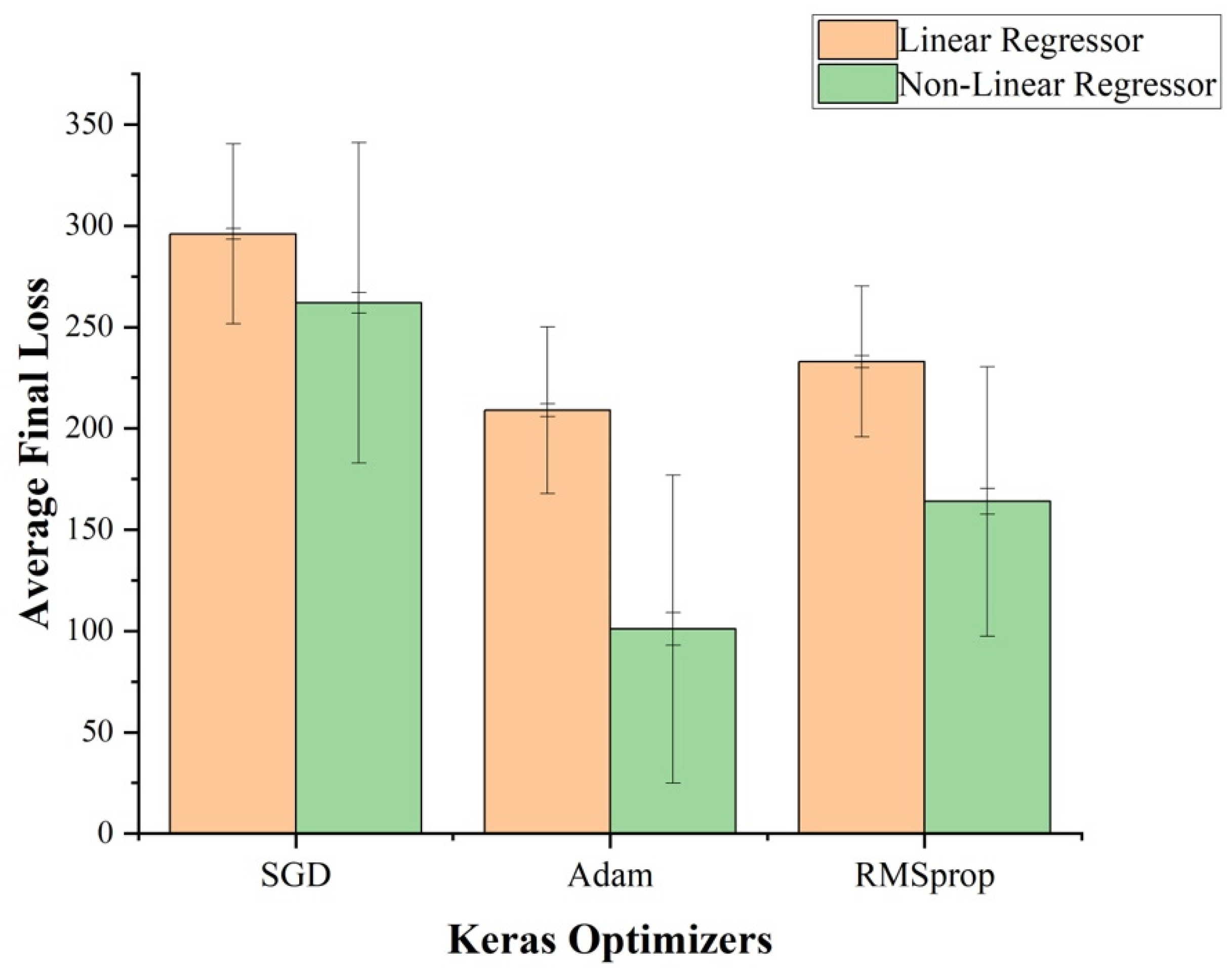
• The linear function for the trained deep neural network on the synthetic dataset was not fully optimized, and the weakest optimizer among them was stochastic gradient descent (SGD), with a mean absolute error of 295.95.
• While iterating for a non-linear algorithm, Adam emerged as the best-performing optimizer, with a loss function of 101.22.
• The proliferation of non-linear neural network algorithms for the prediction and optimization of hydraulic fracture morphology is highly recommended.
• The synthetic data and other conventional data are both suitable for machine learning algorithms and for decisive decision-making procedures. Google TensorFlow libraries present easy access to coding and validation.
• The overall novelty of the study is that it automates data-driven prognosis by optimizing the hydraulic fracture parameters, from complex CMG numerical modeling to using Keras Sequential API algorithms and several optimizer compilations for decision-making analysis.
• This study limits the complexity of physics-driven computational fracking analysis and provides an industrial automation means of predicting the expectations and remedies for fracking petroleum shale reservoirs.

References

1. Irawan, S.; Kinif, B.I.; Bayuaji, R. Maximizing drilling performance through enhanced solid control system. IOP Conf. Ser. Mater. Sci. Eng. 2017, 267, 012038. [Google Scholar] [CrossRef] [Green Version]
2. Irawan, S.; Kinif, I.B. Solid Control System for Maximizing Drilling. Drill. InTech 2018, 1, 192. [Google Scholar] [CrossRef] [Green Version]
3. Gandossi, L. An Overview of Hydraulic Fracturing and Other Formation Stimulation Technologies for Shale Gas Production; no. EUR 26347 EN. 2013; EU Publications: Luxembourg, 2015. [Google Scholar] [CrossRef]
4. Li, G.; Song, X.; Tian, S.; Zhu, Z. Intelligent Drilling and Completion: A Review. Engineering 2022, 18, 33–48. [Google Scholar] [CrossRef]
5. Kundert, D.; Mullen, M. Proper Evaluation of Shale Gas Reservoirs Leads to a More Effective Hydraulic-Fracture Stimulation. In Proceedings of the SPE Rocky Mountain Petroleum Technology Conference, Denver, CO, USA, 14–16 April 2009. [Google Scholar]
6. Liu, Y.; Zheng, X.; Peng, X.; Zhang, Y.; Chen, H.; He, J. Influence of natural fractures on propagation of hydraulic fractures in tight reservoirs during hydraulic fracturing. Mar. Pet. Geol. 2022, 138, 105505. [Google Scholar] [CrossRef]
7. Zhao, H.; Liu, C.; Xiong, Y.; Zhen, H.; Li, X. Experimental research on hydraulic fracture propagation in group of thin coal seams. J. Nat. Gas. Sci. Eng. 2022, 103, 104614. [Google Scholar] [CrossRef]
8. Suo, Y.; Su, X.; Wang, Z.; He, W.; Fu, X.; Feng, F.; Pan, Z.; Xie, K.; Wang, G. A study of inter-stratum propagation of hydraulic fracture of sandstone-shale interbedded shale oil. Eng. Fract. Mech. 2022, 275, 108858. [Google Scholar] [CrossRef]
9. Yang, Y.; Li, X.; Yang, X.; Li, X. Influence of reservoirs/interlayers thickness on hydraulic fracture propagation laws in low-permeability layered rocks. J. Pet. Sci. Eng. 2022, 219, 111081. [Google Scholar] [CrossRef]
10. Xiong, D.; Ma, X. Influence of natural fractures on hydraulic fracture propagation behaviour. Eng. Fract. Mech. 2022, 276, 108932. [Google Scholar] [CrossRef]
11. Wayo, D.D.K.; Irawan, S.; Noor, M.Z.B.M.; Badrouchi, F.; Khan, J.A.; Duru, U.I. A CFD Validation Effect of YP/PV from Laboratory-Formulated SBMDIF for Productive Transport Load to the Surface. Symmetry 2022, 14, 17. [Google Scholar] [CrossRef]
12. Wayo, D.D.K.; Irawan, S.; Khan, J.A.; Fitrianti, F. CFD Validation for Assessing the Repercussions of Filter Cake Breakers; EDTA and SiO2 on Filter Cake Return Permeability. Appl. Artif. Intell. 2022, 36, 2112551. [Google Scholar] [CrossRef]
13. Peng, X.; Rao, X.; Zhao, H.; Xu, Y.; Zhong, X.; Zhan, W.; Huang, L. A proxy model to predict reservoir dynamic pressure profile of fracture network based on deep convolutional generative adversarial networks (DCGAN). J. Pet. Sci. Eng. 2022, 208, 109577. [Google Scholar] [CrossRef]
14. Galkin, S.V.; Martyushev, D.A.; Osovetsky, B.M.; Kazymov, K.P.; Song, H. Evaluation of void space of complicated potentially oil-bearing carbonate formation using X-ray tomography and electron microscopy methods. Energy Rep. 2022, 8, 6245–6257. [Google Scholar] [CrossRef]
15. Ponomareva, I.N.; Martyushev, D.A.; Govindarajan, S.K. A new approach to predict the formation pressure using multiple regression analysis: Case study from Sukharev oil field reservoir—Russia. J. King Saud Univ.-Eng. Sci. 2022, in press. [Google Scholar] [CrossRef]
16. Wang, D.B.; Zhou, F.-J.; Li, Y.-P.; Yu, B.; Martyushev, D.; Liu, X.-F.; Wang, M.; He, C.-M.; Han, D.-X.; Sun, D.-L. Numerical simulation of fracture propagation in Russia carbonate reservoirs during refracturing. Pet. Sci. 2022, 19, 2781–2795. [Google Scholar] [CrossRef]
17. Bessmertnykh, A.; Dontsov, E.; Ballarini, R. The effects of proppant on the near-front behavior of a hydraulic fracture. Eng. Fract. Mech. 2020, 235, 107110. [Google Scholar] [CrossRef]
18. Yi, S.S.; Wu, C.H.; Sharma, M.M. Proppant distribution among multiple perforation clusters in plug-and-perforate stages. SPE Prod. Oper. 2018, 33, 654–665. [Google Scholar] [CrossRef]
19. Suri, Y.; Islam, S.Z.; Hossain, M. Proppant transport in dynamically propagating hydraulic fractures using CFD-XFEM approach. Int. J. Rock Mech. Min. Sci. 2020, 131, 104356. [Google Scholar] [CrossRef]
20. Wu, C.H.; Sharma, M.M. Modeling proppant transport through perforations in a horizontal wellbore. SPE J. 2019, 24, 1777–1789. [Google Scholar] [CrossRef]
21. Wang, K.; Zhang, G.; Du, F.; Wang, Y.; Yi, L.; Zhang, J. Simulation of directional propagation of hydraulic fractures induced by slotting based on discrete element method. Petroleum 2022, in press. [Google Scholar] [CrossRef]
22. Luo, A.; Li, Y.; Wu, L.; Peng, Y.; Tang, W. Fractured horizontal well productivity model for shale gas considering stress sensitivity, hydraulic fracture azimuth, and interference between fractures. Nat. Gas Ind. B 2021, 8, 278–286. [Google Scholar] [CrossRef]
23. Martyushev, D.A.; Ponomareva, I.N.; Filippov, E.V. Studying the direction of hydraulic fracture in carbonate reservoirs: Using machine learning to determine reservoir pressure. Pet. Res. 2022, in press. [Google Scholar] [CrossRef]
24. Dong, Z.; Wu, L.; Wang, L.; Li, W.; Wang, Z.; Liu, Z. Optimization of Fracturing Parameters with Machine-Learning and Evolutionary Algorithm Methods. Energies 2022, 15, 6063. [Google Scholar] [CrossRef]
25. Elbaz, K.; Shen, S.L.; Zhou, A.; Yin, Z.Y.; Lyu, H.M. Prediction of Disc Cutter Life During Shield Tunneling with AI via the Incorporation of a Genetic Algorithm into a GMDH-Type Neural Network. Engineering 2021, 7, 238–251. [Google Scholar] [CrossRef]
26. Shen, S.L.; Elbaz, K.; Shaban, W.M.; Zhou, A. Real-time prediction of shield moving trajectory during tunnelling. Acta Geotech. 2022, 17, 1533–1549. [Google Scholar] [CrossRef]
27. Elbaz, K.; Yan, T.; Zhou, A.; Shen, S.L. Deep learning analysis for energy consumption of shield tunneling machine drive system. Tunn. Undergr. Space Technol. 2022, 123, 104405. [Google Scholar] [CrossRef]
28. Fang, J.; Gong, B.; Caers, J. Data-Driven Model Falsification and Uncertainty Quantification for Fractured Reservoirs. Engineering 2022, 18, 116–128. [Google Scholar] [CrossRef]
29. Aboosadi, Z.A.; Rooeentan, S.; Adibifard, M. Estimation of subsurface petrophysical properties using different stochastic algorithms in nonlinear regression analysis of pressure transients. J. Appl. Geophy. 2018, 154, 93–107. [Google Scholar] [CrossRef]
30. Kingma, D.P.; Ba, J. Adam: A Method for Stochastic Optimization. 2014. Available online: http://arxiv.org/abs/1412.6980 (accessed on 7 January 2023).
31. Kamrava, S.; Tahmasebi, P.; Sahimi, M. Enhancing images of shale formations by a hybrid stochastic and deep learning algorithm. Neural Netw. 2019, 118, 310–320. [Google Scholar] [CrossRef]
32. Wang, Q.; Song, Y.; Zhang, X.; Dong, L.; Xi, Y.; Zeng, D.; Liu, Q.; Zhang, H.; Zhang, Z.; Yan, R.; et al. Evolution of corrosion prediction models for oil and gas pipelines: From empirical-driven to data-driven. Eng. Fail. Anal. 2023, 146, 107097. [Google Scholar] [CrossRef]
33. Liu, Y.Y.; Ma, X.H.; Zhang, X.W.; Guo, W.; Kang, L.X.; Yu, R.Z.; Sun, Y.P. A deep-learning-based prediction method of the estimated ultimate recovery (EUR) of shale gas wells. Pet. Sci. 2021, 18, 1450–1464. [Google Scholar] [CrossRef]
34. A Comprehensive Guide on Deep Learning Optimizers. Available online: https://www.analyticsvidhya.com/blog/2021/10/a-comprehensive-guide-on-deep-learning-optimizers/ (accessed on 10 February 2023).
35. Mohapatra, R.; Saha, S.; Coello, C.A.C.; Bhattacharya, A.; Dhavala, S.S.; Saha, S. AdaSwarm: Augmenting Gradient-Based Optimizers in Deep Learning with Swarm Intelligence. IEEE Trans. Emerg. Top Comput. Intell. 2022, 6, 329–340. [Google Scholar] [CrossRef]
36. Hou, L.; Elsworth, D.; Zhang, F.; Wang, Z.; Zhang, J. Evaluation of proppant injection based on a data-driven approach integrating numerical and ensemble learning models. Energy 2023, 264, 126122. [Google Scholar] [CrossRef]
37. Mukhtar, F.M.; Duarte, C.A. Coupled multiphysics 3-D generalized finite element method simulations of hydraulic fracture propagation experiments. Eng. Fract. Mech. 2022, 276, 108874. [Google Scholar] [CrossRef]
38. Pezzulli, E.; Nejati, M.; Salimzadeh, S.; Matthäi, S.K.; Driesner, T. Finite element simulations of hydraulic fracturing: A comparison of algorithms for extracting the propagation velocity of the fracture. Eng. Fract. Mech. 2022, 274, 108783. [Google Scholar] [CrossRef]
39. Ou, C.; Liang, C.; Li, Z.; Luo, L.; Yang, X. 3D visualization of hydraulic fractures using micro-seismic monitoring: Methodology and application. Petroleum 2022, 8, 92–101. [Google Scholar] [CrossRef]
40. Ortiz, D.A.A.; Klimkowski, L.; Finkbeiner, T.; Patzek, T.W. The effect of hydraulic fracture geometry on well productivity in shale oil plays with high pore pressure. Energies 2021, 14, 7727. [Google Scholar] [CrossRef]
41. Zhang, Y.; Liu, Z.; Han, B.; Zhu, S.; Zhang, X. Numerical study of hydraulic fracture propagation in inherently laminated rocks accounting for bedding plane properties. J. Pet. Sci. Eng. 2022, 210, 109798. [Google Scholar] [CrossRef]
42. Kulga, B.; Artun, E.; Ertekin, T. Development of a data-driven forecasting tool for hydraulically fractured, horizontal wells in tight-gas sands. Comput. Geosci. 2017, 103, 99–110. [Google Scholar] [CrossRef]
43. Yusof, M.A.M.; Mahadzir, N.A. Development of mathematical model for hydraulic fracturing design. J. Pet. Explor. Prod. Technol. 2015, 5, 269–276. [Google Scholar] [CrossRef] [Green Version]
44. Nguyen, H.T.; Lee, J.H.; Elraies, K.A. A review of PKN-type modeling of hydraulic fractures. J. Pet. Sci. Eng. 2020, 195, 107607. [Google Scholar] [CrossRef]
45. Wypych, G. The Effect of Fillers on the Mechanical Properties of Filled Materials. In Handbook of Fillers, 5th ed.; ChemTech Publishing: Toronto, ON, Canada, 2021; pp. 525–608. [Google Scholar] [CrossRef]
46. Fanchi, J.R. Fluid Flow Equations. In Shared Earth Modeling; Gulf Professional Publishing: Houston, TX, USA, 2002; pp. 150–169. [Google Scholar] [CrossRef]
47. Fanchi, J.R. Reservoir Simulation. In Integrated Reservoir Asset Management; Elsevier: Amsterdam, The Netherlands, 2010; pp. 223–241. [Google Scholar] [CrossRef]
48. PKN Hydraulic Fracturing Model—FrackOptima Help. Available online: http://www.frackoptima.com/userguide/theory/pkn.html (accessed on 21 February 2023).
49. Nordgren, R.P. Propagation of a Vertical Hydraulic Fracture. Soc. Pet. Eng. J. 1972, 12, 306–314. [Google Scholar] [CrossRef]
50. Rahman, M.M.; Rahman, M.K. A review of hydraulic fracture models and development of an improved pseudo-3D model for stimulating tight oil/gas sand. Energy Sources Part A Recovery Util. Environ. Eff. 2010, 32, 1416–1436. [Google Scholar] [CrossRef]
51. Misra, S.; Li, H. Deep neural network architectures to approximate the fluid-filled pore size distributions of subsurface geological formations. In Machine Learning for Subsurface Characterization; Elsevier: Amsterdam, The Netherlands, 2019; pp. 183–217. [Google Scholar] [CrossRef]
52. Duru, U.I.; Wayo, D.D.K.; Oguh, R.; Cyril, C.; Nnani, H. Computational Analysis for Optimum Multiphase Flowing Bottom-Hole Pressure Prediction. Transylv. Rev. 2022, 30, 16010–16023. Available online: http://transylvanianreviewjournal.com/index.php/TR/article/view/907 (accessed on 20 February 2023).
53. Kim, Y.; Satyanaga, A.; Rahardjo, H.; Park, H.; Sham, A.W.L. Estimation of effective cohesion using artificial neural networks based on index soil properties: A Singapore case. Eng. Geol. 2021, 289, 106163. [Google Scholar] [CrossRef]
Figure 1. Extended finite element method (XFEM) showing its initial pressure for fracturing, adapted with permission from Ref. [19], 2020, Suri, Y.
Bdcc 07 00057 g001
Figure 2. Fracture propagation perpendicular to the slotting in sample 4 adapted with permission from Ref. [21], 2022, Wang, K.
Bdcc 07 00057 g002
Figure 3. Coefficient of correlation (a) before DHF, (b) after DHF, adapted with permission from Ref. [23], 2022, Martyushev, D.A.
Bdcc 07 00057 g003
Figure 4. EOA-PSO with the highest NPV, adapted with permission from Ref. [24], 2022, Dong, Z.
Bdcc 07 00057 g004
Figure 5. Optimizers performances, adapted with permission from Ref. [34].
Bdcc 07 00057 g005
Figure 6. Flowchart for optimizing hydraulic fracturing.
Bdcc 07 00057 g006
Figure 8. Illustrative Perkins–Kern–Nordgren one-wing fracture model.
Bdcc 07 00057 g008
Figure 9. Scattered raw data validation for proppant propagation.
Bdcc 07 00057 g009
Figure 10. Height/Pwf loss curves; (a) SGD final loss = 61.50, (b) Adam final loss = 125.86, (c) RMSprop final loss = 231.91.
Bdcc 07 00057 g010
Figure 11. Porosity/Pwf loss curves; (a) SGD final loss = 399.11, (b) Adam final loss = 65.46, (c) RMSprop final loss = 106.36.
Bdcc 07 00057 g011
Figure 12. Length/Pwf loss curves; (a) SGD Final loss = 366.46, (b) Adam final loss = 155.50, (c) RMSprop final loss = 174.33.
Bdcc 07 00057 g012
Figure 13. Width/Pwf loss curves; (a) SGD final loss = 620.66, (b) Adam final loss = 93.45, (c) RMSprop final loss = 124.99.
Bdcc 07 00057 g013
Figure 14. Permeability/Pwf loss curves; (a) SGD final loss = 61.50, (b) Adam final loss = 72.6, (c) RMSprop Final loss = 169.38.
Bdcc 07 00057 g014
Figure 15. Conductivity/Pwf loss curves; (a) SGD final loss = 61.72, (b) Adam final loss = 94.42 (c) RMSprop final loss = 177.10.
Bdcc 07 00057 g015
Figure 16. Fracture height linear regressor model and optimizer performances; (a) SGD final loss = 347.88, (b) Adam final loss = 221.07, (c) RMSprop final loss = 220.25.
Bdcc 07 00057 g016
Figure 17. Porosity linear regressor model and optimizer performances; (a) SGD final loss = 225.58, (b) Adam final loss = 234.23, (c) RMSprop final loss = 225.56.
Bdcc 07 00057 g017
Figure 18. Permeability linear regressor model and optimizer performances; (a) SGD final loss = 260.98, (b) Adam final loss = 255.49, (c) RMSprop final loss = 253.81.
Bdcc 07 00057 g018
Figure 19. Fracture length linear regressor model and optimizer performances; (a) SGD final loss = 487.19, (b) Adam final loss = 157.91, (c) RMSprop final loss = 253.81.
Bdcc 07 00057 g019
Figure 20. Fracture width linear regressor model and optimizer performances; (a) SGD final loss = 255.78, (b) Adam final loss = 251.87, (c) RMSprop final loss = 249.91.
Bdcc 07 00057 g020
Figure 21. Optimizing Keras optimizers at different final losses.
Bdcc 07 00057 g021
Figure 22. Fracture conductivity validation.
Bdcc 07 00057 g022