1. Introduction
Football, the world’s most popular game with a fan following of over 3.5 billion, is a highly unpredictable, competitive and physically demanding sport [
1]. The score-line can change at any given point of time and there are many matches where goals were scored during extra time, which resulted in the match results turning upside down. This high unpredictability is one of the reasons why football is the world’s most popular game. In a football match, on-field players can be substituted by off-field players and the match continues without any interruption [
2]. This is one important method by which the team strategy can be altered in an ongoing match.
As mentioned above, player substitution provides a way for the team to change their on-field tactics and game plan while a match is in progress [
3]. There is very minimal research conducted on ways to maximize the game advantage by means of introducing tactical player substitution in football matches. Machine Learning (ML) can be used to predict the most effective player to be substituted at any given time, based on live game statistics and real-time match data [
4]. This has immense scope for implementation and improvement in the current understanding of player substitution and end-result prediction. Conducting further research works in this area and accurately predicting player substitutions using ML models can provide team managers great confidence in planning team combinations and strategies.
At present, the team manager takes decisions based on instinct when player substitution is needed [
5]. In most cases, wrong substitution and timing of substitution have led to a negative impact, leading to an unfavorable match result. There is a lack of effective software which can provide heads-up to the coach/team manager about the possibility of a perfect substitution for achieving a significant game advantage. There is also a lack of confidence in using software due to a lack of solid research papers on the utilization of machine learning on substitution data [
6]. Statistical data from past Football matches including match events like the scoring goal, ball passing details, shots taken, substitutions, and injury with the time of the event are available in the public domain. This historical data, if taken for analytics, can yield a significant advantage when players are selected for substitution.
The purpose of this research is to explore the potential of employing machine learning algorithms to predict substitutions in Football, and how it could influence the outcome of a match. By collecting and analyzing historical data on game statistics, player substitution, substitution timing, playing position, and match result, this study seeks to reveal a correlation [
5] between the timing of substitutions, the score at the time of substitution, the final score of the match [
7], and the prediction of substitution [
8].
Although football is a highly popular game, so far, no intelligent tool has been reported in the literature to assist coaches in making strategic decisions for substitution. This research work aims to determine which players should not be substituted so that any advantage gained is not lost. It can be used to make all three allowed substitutions, including double substitutions, and time them accurately to maximize the benefit. The main contributions have been provided as follows.
A unique approach based on machine learning models is developed in this research work, which can be used to predict the most appropriate substitute-player, in live football matches based on historical data. This can be used by football teams to gain tactical match advantage and potentially alter the outcome of the match. In this proposed work, an attempt is made to identify the research gaps and come up with solid data to demonstrate that tactical and timely substitution prediction using machine learning models, can have a great impact on the game strategy and hence influence the match result.
51,738 substitutions from 9074 European league matches in 5 leagues spanning across 6 seasons were analyzed using the proposed ML-based approach.
From the dataset, a huge number of events for example, almost 1 million, substitution data and goal score data were programmatically filtered out and substitutions were marked positive or negative based on the event timestamps. This extracted dataset can also be used as a base for future studies.
Six ML techniques were identified across different machine learning models from the state-of-the-art and conducted their performance comparison to choose the appropriate ML model based on their prediction accuracies.
The novelty of this work lies in formulating the problem of predicting the substitution of football players in live matches and appropriate data manipulation from a large number of unorganized datasets to generate an effective solution.
The rest of the paper is organized as follows.
Section 2 describes the existing research papers which discuss player substitutions in football matches.
Section 3 illustrates the methodology to predict substitution and ML techniques.
Section 4 presents the experiments conducted and the analysis of the final results. This section also presents a discussion on the model validation, performance comparison with the ML techniques used and their limitations. Conclusions and future research directions are outlined in
Section 5.
2. Background Literature
There are only a few research papers, which analyze substitution data to prove their hypothesis. The work proposed by Miguel et al. [
9], analyses the team centroid, before and after each player substitution and discusses how it affects the team’s tactical behaviour. Their research utilized a sample of 659 substitutions from 234 matches in the German Bundesliga. Data was collected from an optical tracking system [
10] for the segments before and after the substitution, which was then employed to analyse and draw conclusions. Statistical analysis was conducted using the R software [
11], while computations were performed in Python [
12]. The research paper concludes that when an attacking player is substituted, the team’s centroid shifts to a more advanced position, increasing the chances of scoring. Conversely, a defensive substitution shifts the team centroid to a defensive position, which could be beneficial when the team is leading and needs to protect its lead. However, the work does not analyse the effect of the substitutions on the match result, identify the degree of impact they have on the game, or predict the optimal time to make substitutions. In the proposed work, an attempt has been made to address this gap.
Rey et al. [
13] have presented the impact of situational variables [
14] on the tactics and timing of football substitutions being analysed. This paper recommends that the coaches consider the optimal time to make their first, second, and third substitutions, depending on whether their team is behind, tied, or ahead. The authors used a sample from the 2013–2014 UEFA Champions League consisting of 677 substitutions from 124 matches for their analysis. Statistical analysis was conducted on the dataset and the DT algorithm J48 [
15] in WEKA [
16] was used to identify the optimal time for substitutions. Their work offers recommendations for the substitutions, however, it does not predict the match outcome based on these substitutions. An attempt is made to address this research gap in this proposed work.
An ML approach to support substitutions is presented in [
17], the real-time physical performance of football players during the match is analysed and this is suggested as an additional parameter, to decide on the substitutions. The authors used data from 302 football matches to develop an ML model. Multi-camera positional systems and Sports VU optical tracking systems [
10] were used to track the real-time motion data of players, and variables such as distance covered, acceleration, deceleration, metabolic power, and energy expenditure of players [
18] were analysed in real time. The physical performance analysis of individual players provided the coaches with an insight into their physical decline and suggested substituting the on-field players. However, the research does not recommend who should be substituted in place of the player in decline, nor does it take historical data into account. However, the proposed work has attempted to address this research gap.
Stock et al. [
19] extended a stochastic model for football leagues based on the team’s potential for predicting the tournament’s outcome by using the market value or/and the ongoing team’s performance. An agent-based model was proposed in their work, where N teams play against each other, and the team’s potential is incremented or decremented based on simulated championships. However, the authors in their research have not taken into account the performance of individual players and how they contributed when substituted.
Based on the critical analysis of the above research works, it was identified that the existing models failed to predict which player should be substituted based on the team’s current performance, whether they are ahead, tied, or behind. None of the research used ML models to analyse and determines whether the substitutions had a positive or negative impact on the match result. This proposed work seeks to bridge this gap by determining if the substitution was positive or negative based on the score line and predicting whether the player chosen for substitution will have a positive or negative effect.
3. Research Methodology
The official FIFA website [
20] captures most of the historical football data and makes it available for public research purposes. Other websites also provide data stored from major league football matches, which is available for research. For this study, data from Kaggle [
21] was collected and analyzed. The dataset includes information from 9074 games, totaling 941,009 events from five European football leagues, namely England, Spain, Germany, Italy, and France, spanning from the 2011/2012 to 2016/2017 seasons. The data is organized into three files: ‘events.csv’, which contains details about the events that occurred in the games; ‘dictionary.txt’, which describes the events mentioned in the ‘events.csv’ file; and ‘ginf.csv’, which provides information about each game.
For analyzing and manipulating the data, Python 3.10 [
12] was utilized, and the scikit-learn package 1.1.0 [
22] was used for constructing the ML models. The Pandas [
23] module in Python was used to work with the dataset, and because the data was largely numerical, quantitative analysis [
24] was used extensively. Python scripts utilizing ML models were written to examine the substitution timings and the impact of the substituted player on the game, and Jupyter Notebook [
25] was used to create, edit, and debug the scripts.
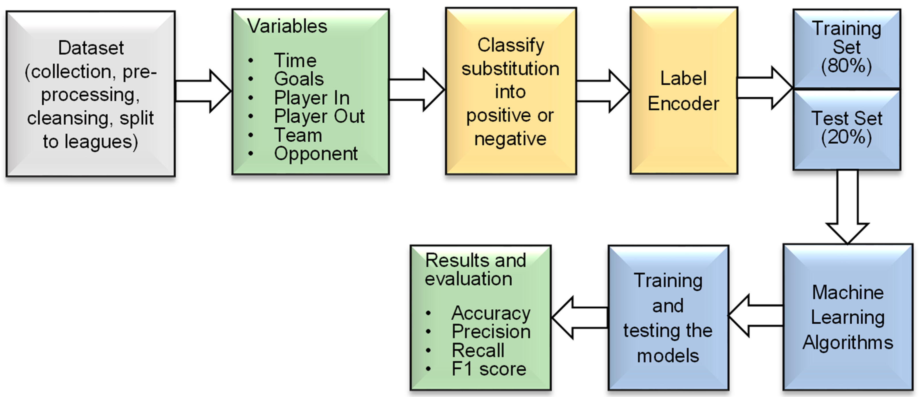
The Python scripts were uniquely designed and developed to manipulate the data obtained from an open-access database. These scripts were created to analyze the dataset entries and detect all the events from individual games. Once the events from each game were identified, the effectiveness of player substitutions was determined programmatically by examining the goal scoreline before substitutions and the goal scoreline at the end of the match. This process was performed for every substitution, and the resulting values were used to construct supervised machine-learning models using the Python sci-kit-learn module. As a result, well-known machine learning algorithms were applied in the sports domain, which is not commonly performed. This has the potential to make a significant impact on the widely popular sport. The innovative approaches to data collection, design, manipulation, and implementation can pave the way for future research. The detailed steps of technical work are presented in
Figure 1.
3.1. Data Preprocessing
Data acquired from various sources may contain unwanted or irrelevant information. Data cleansing is the process of modifying the data according to the research requirements [
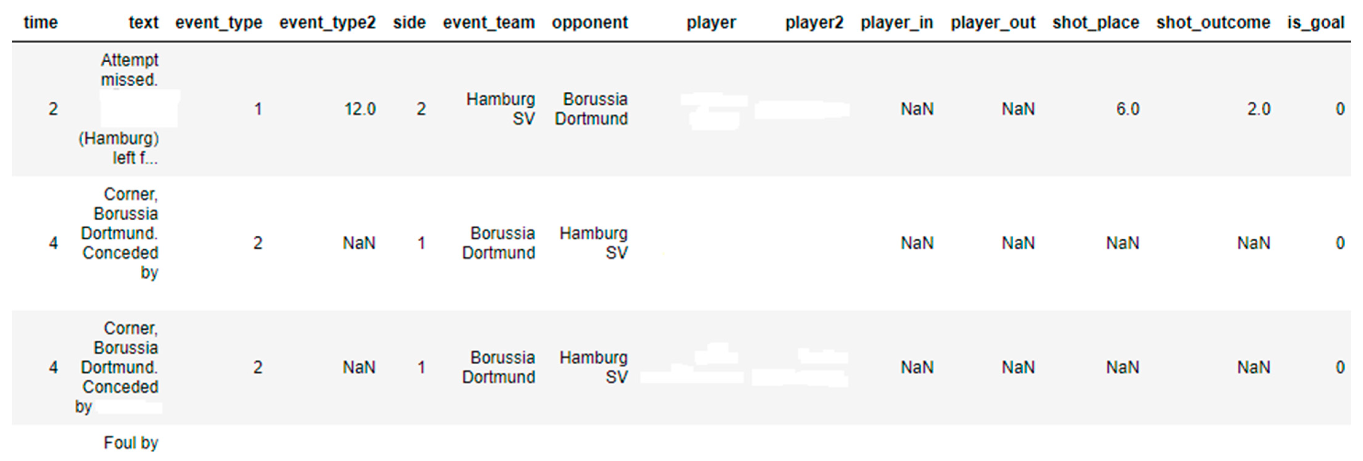
26]. The ‘events.csv’ and ‘ginf.csv’ datasets were combined to include the league country names in each event. To conduct the analysis, the data from the different leagues were separated. Analyzing all 941,009 events together was not a viable option, as the substitution data would not be meaningful when applied to the ML models [
4]. Consequently, the dataset was divided into five subsets, one for each league, based on the league country. After splitting, each dataset contained data from six seasons of a single European league. A sample of the pre-processed dataset is presented in
Figure 2.
3.2. Data Manipulation
To determine if a particular substitution had a positive or negative effect on the result of the game, the number of goals scored and conceded by each team was recorded and stored. A new column called ‘positive_sub’ was added to the Python panda’s data frame [
23]. For each match, the timestamps of each goal scored by each team were stored separately.
To identify if a player substitution had a positive or negative impact on the game, the timestamp of the substitution was taken. The goal difference before the substitution and the goal difference at the end of the game were then compared. If the goal difference at the end of the game was in favour of the opposition team, the substitution was considered negative, and the ‘positive_sub’ column was updated with a value of ‘0’.
If the goal difference remained the same or the goal difference was in favour of the team the player was substituted into, the substitution was considered positive, and the ‘positive_sub’ column was updated with a value of ‘1’.
All the substitutions were analysed programmatically in the same way and the value in the ‘positive_sub’ column was updated using Python Panda’s data frame manipulation techniques.
The dataset includes an attribute called ‘is_goal’ which indicates whether an event led to a goal. To analyse events for a particular game, they were filtered and sorted based on the ‘time’ attribute using Python’s pandas’ data frame manipulation techniques. The goal scoreline was determined by tallying the goals scored by each team, allowing us to determine the scoreline when a player was substituted and the final scoreline at the end of the match. If the scoreline improved after the player was substituted (as indicated by the ‘player_in’ descriptor), the substitution was considered positive. It can be seen that a few fields in
Figure 2 with ‘NaN’. Using Python Panda’s module data manipulation techniques, ‘NaN’ was discarded, and the final dataset is shown in
Figure 3 in the next section.
As illustrated in
Figure 1, the input variables selected from the dataset to generate the machine learning models primarily included: ‘time’ (event time), ‘event_team’ (substituting player’s team name), ‘opponent’ (opponent team name), ‘player_in’ (substituted-in player), and ‘player_out’ (substituted-out player). These variables were chosen based on the assumption that they have the potential to have the greatest influence on the outcome of the match. The variable ‘goal’ was utilized to programmatically determine the introduction of the ‘positive_sub’ variable.
3.3. Data Masking
To protect the identity [
27] of the players, data masking techniques [
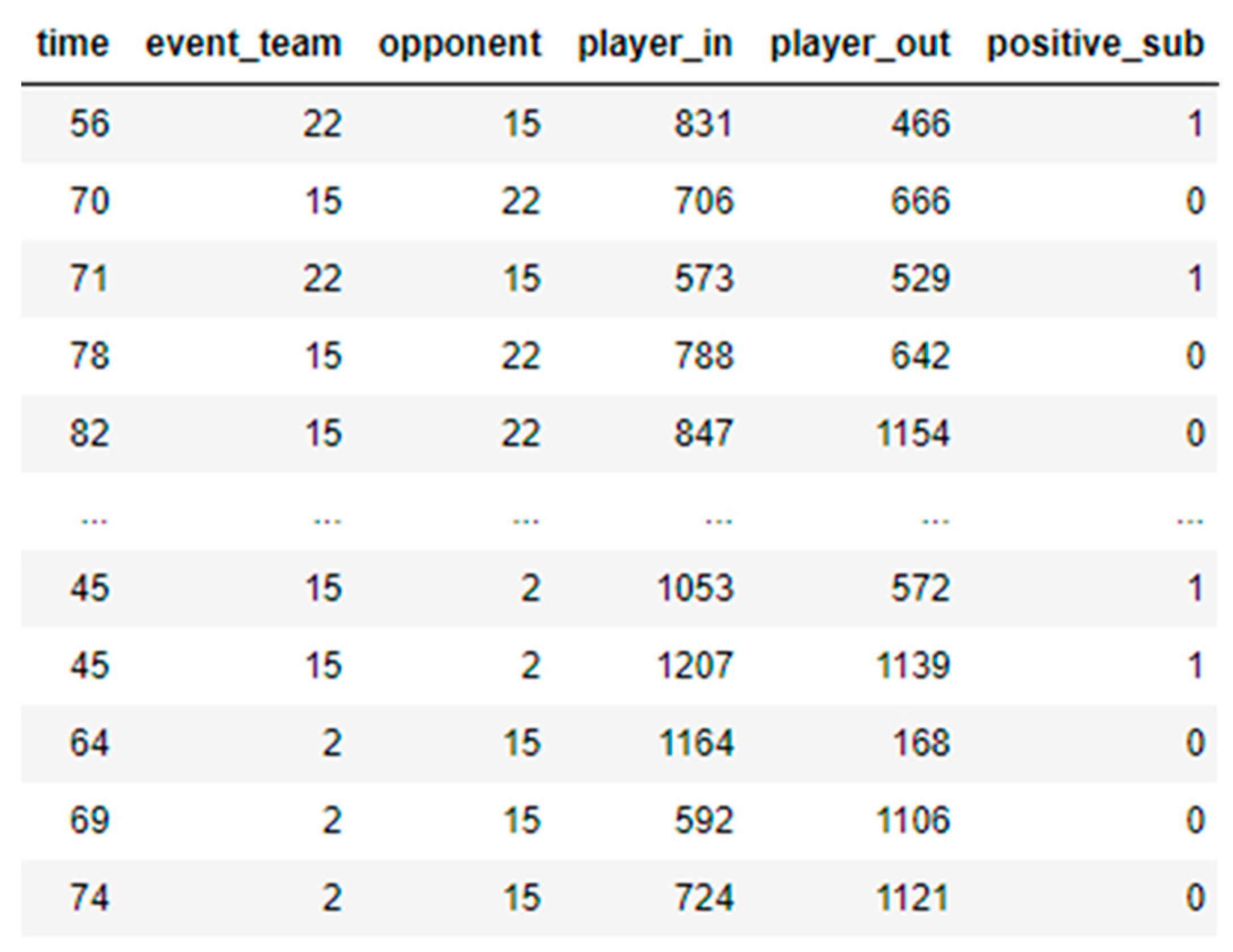
28] were used to replace the names of the players with numbers. The Python module ‘LabelEncoder’ was used to assign a unique number to each player. For example, in the France league data from the four seasons, 1277 players were substituted in a total of 2076 matches, for a total of 11,576 substitutions. To ensure confidentiality, the names of the substitute players were masked with unique numbers using data masking and label encoding methods.
Figure 3 presents a sample of the manipulated and masked data.
3.4. Train–Testsplit
The entire dataset was randomly split into train data and test data. The train data was used to train the models while the test data was used to test the models generated [
29]. The train-test split was at 80:20. With the same split, when the model was trained again and again, almost consistent results were obtained with the test data, suggesting that the train-test split was effectively identified.
3.5. Machine Learning Models
The supervised ML techniques outlined in the following subsections were used to predict the substitutions, which had already been evaluated and labelled as either ‘positive’ or ‘negative’ based on the result of the match [
4]. The Python sci-kit-learn module was employed to both implement and evaluate these models [
22].
3.5.1. Logistic Regression (LR)
LR [
30] is employed to analyze the binary or proportional output of one or more inputs. This research attempts to predict whether a substitution has a positive or negative effect based on a variety of factors, including the in-player (the player substituted in), the out-player (the player substituted out), the goal score line, the substitution time, the team’s name, and the opposition team name. The basic linear regression hypothesis function can be expressed by Equation (1).
where
x is the input training data,
y is the predicted output,
is the intercept, and
is the coefficient. The best regression fit is obtained by finding the optimal values for
and
.
3.5.2. Decision Tree Regression
The dataset is divided into smaller subsets and a DT is constructed step by step with decision nodes and leaf nodes [
31]. In this research, a DT is incrementally developed based on the input parameters, and the result of the player substitution is calculated accordingly.
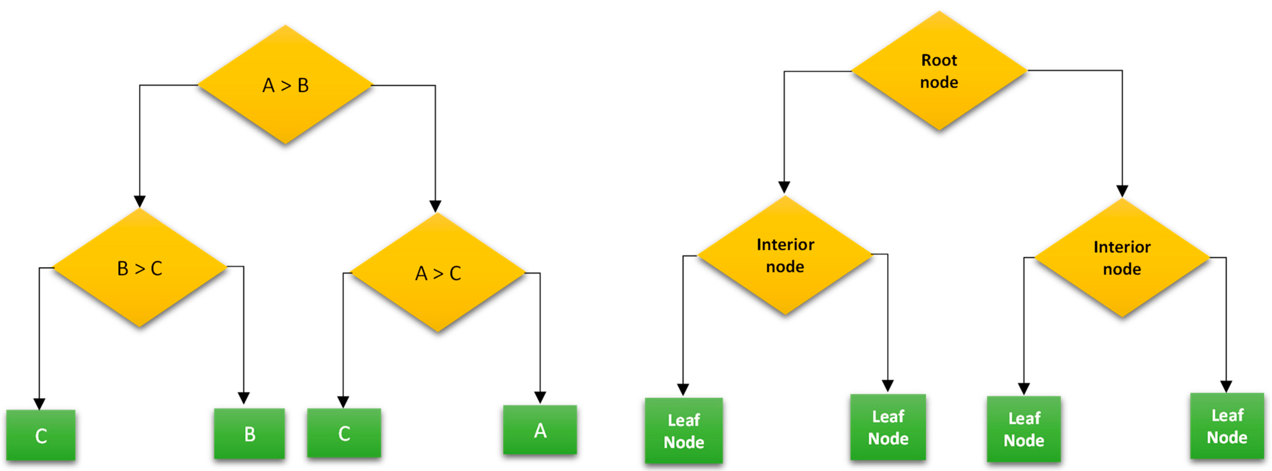
The dataset was first split to train data (80%) and test data (20%). DT model was then built using the sci-kit-learn python module by defining the predictor (time, player name, team name, etc.) and target values (positive_sub). Predictions were performed on the test data using the learned relationship between predictor and target values. The performance of the model was analyzed based on the results obtained on the final predicted values. The architecture of DT is presented in
Figure 4.
In
Figure 4, The yellow boxes indicate decision nodes, which are features of the dataset, while the green box represents the leaf node, which represents the outcome. The decision tree model has three possible outcomes: A, B, and C. The outcome is determined by the features mentioned as interior nodes in the dataset.
3.5.3. K-Nearest Neighbor Regression
The K-Nearest Neighbor method was used to determine the similarity between new data and existing data, and then classified the input into the most similar category presented in [
32]. In this research, two centroids were selected (one for positive and one for negative), and the new data was continually classified into the appropriate category based on the existing data. The distance between the new data and the nearest neighbors was calculated using the Euclidean distance formula [
33].
Euclidean distance between two data points
A (
x1,
y1) and
B (
x2,
y2) is calculated as presented in Equation (2).
3.5.4. Support Vector Machine (SVM)
The SVM learning method maps the training data points into a new space, with the goal of maximizing the distance between them [
34]. Subsequent training data points are then mapped into the same space and their classifications are determined based on their position in the space.
In this work, “positive_sub” predictions were performed on the test data using the learned relationship between predictor and target values. The performance of the model was analyzed based on the results obtained on the final predicted values.
Given a set of training data points (
x_1,
y_1), (
x_2,
y_2), …, (
x_n,
y_n) where
x_i is a d-dimensional feature vector and
y_i is the corresponding label, the goal is to find the hyperplane
w and bias
b that maximize the margin between the two classes and for
i = 1, 2, …,
n (Equation (3)). The margin is defined as the distance between the closest training data points of the two classes and the hyperplane.
3.5.5. Multinomial Naïve Bayes
The MNB algorithm is widely used in Natural Language Processing, with predictions based on tag labels [
35]. This algorithm leverages tag labels to inform its predictions. The formula for Bayes’ theorem is shown in Equation (4).
where
P(
class|
features) is the posterior probability of the class given the features,
P(
features|
class) is the probability of the features given the class,
P(
class) is the probability of the class occurring in the training data, and
P(
features) is the probability of the features occurring in the training data. The posterior probability of each class (positive_sub) was calculated, given the features of the new data point and choose the value with the highest probability.
3.5.6. Random Forest Classifier
The RF classifier [
36] works by dividing the dataset into several small decision trees, which are then combined to form an ensemble [
37] that can make more accurate predictions. A large number of decision trees are trained on different subsets of the training data, and the final prediction is made by averaging the predictions of all the individual decision trees. This is performed by selecting a random subset of the features for each DT and training the tree on the corresponding subset of the training data. The predictions of all the individual trees are then combined to make the final prediction. The use of multiple decision trees and the random selection of features for each tree helps to reduce overfitting, as the individual trees are less likely to be overfitting to the training data. This results in a more robust and accurate model.
3.6. Perfromnaces Matrices
The test set can result in four possible outcomes: True Positive (Prediction is Positive and the result is Positive), True Negative (Prediction is Negative and the result is Negative), False Positive (Prediction is Positive but the result is Negative), and False Negative (Prediction is Negative but the result is Positive). Based on the number of entries predicted, the Accuracy [
38], Precision & Recall [
39], F1-Score [
40], and Confusion Matrix [
41] of the ML models can be evaluated by the following subsections.
3.6.1. Accuracy
The accuracy of the model can be determined by taking the number of correct predictions and dividing it by the total number of predictions made (Equation (5)). If all of the predictions are correct, then the accuracy of the model is expected to be 100%. This means that all the predictions must be either true positives or true negatives, with no false predictions.
In this work, the value ‘positive_sub’ predicts if the substitution created a positive impact or negative impact. For example, the accuracy of LR on test data was 70%, which means that the model was able to predict 70 instances of ‘positive_sub’ correctly in the test data and 30 predictions were incorrect on a sample of 100 test data entries. Accuracy is a useful metric for evaluating the performance of ML models, however, it can be misleading if the classes in the dataset are imbalanced. For example, if the dataset has 95% of “positive_sub” as ‘1’ and only 5% as ‘0’, then a model that always predicts “1” would have an accuracy of 95%, even though it is not making any correct prediction. In this case, other metrics such as precision, recall, and F1 score, explained in the following sections, should be considered to obtain better output-related information.
3.6.2. Precision
Precision is the proportion of true positives among all the predictions labeled as positive [
39]. This is calculated by taking the number of true positives and dividing it by the sum of true positives and false positives and presented by Equation (6).
True positive predictions are instances where the model correctly predicts the positive value (e.g., “positive_sub” actual value is ‘1’ and the predicted value is also ‘1’, in our case). False positive predictions are instances where the model incorrectly predicted the positive value. Precision is often used in conjunction with another metric called recall, explained in the next section. Precision and recall can be used to evaluate the performance of a model in a classification task. A high precision means that the model is good at identifying the positive class and a low precision means that it is also mislabeling a lot of negative instances as positive.
3.6.3. Recall
The recall is a measure of the ability of a model to identify all the positive instances in a dataset [
39]. It is defined as the number of true positive predictions made by the model, divided by the total number of actual positive instances in the dataset. This is calculated by dividing True Positive by the sum of True Positive and False Negatives. The formula for the recall is shown in Equation (7).
True positive predictions are instances where the model correctly predicts the positive class (e.g., “positive_sub” actual value is ‘1’ and the predicted value is also ‘1’, in our case). False negative predictions are instances where the model incorrectly predicts the negative class (e.g., “positive_sub” actual value is ‘1’ but the predicted value is ‘0’, in our case). A high recall means that the model performs well at finding all the positive instances, whereas a low recall indicates missing a lot of the positive instances.
3.6.4. F1 Score
F1 Score is normally defined as a harmonic mean of Precision and Recall values [
40]. Equation (8) is the formula for calculating the F1 score.
F1 score is high if Precision and Recall are high and the opposite while their score is low. The F1 score combines Precision and Recall into a single score, and it is sensitive to changes in both precision and recall. The F1 score is only meaningful when the positive and negative classes are balanced. If the dataset is imbalanced, the F1 score may not be an informative metric, and it may be more useful to look at precision and recall separately.
4. Results and Discussion
This section analyses the results obtained from the ML models. Data analysis, manipulation and graph plotting were performed using Python 3.x [
12] using various Python modules like pandas, NumPy, and matplotlib [
42].
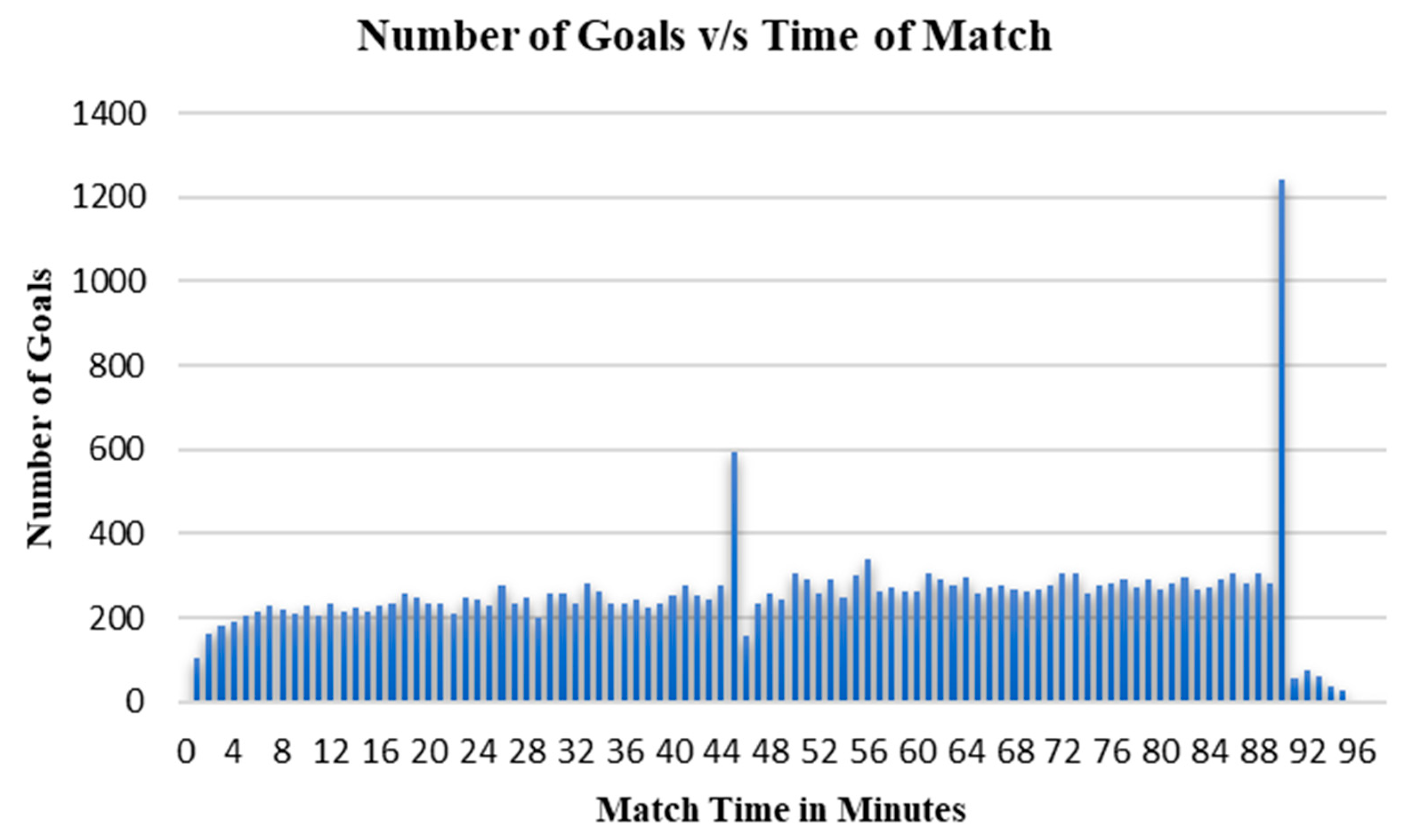
4.1. Analysis of Goals Scored vs. Time
An analysis of the goals scored in the German league showed that the number of goals scored per minute was relatively steady throughout the duration of the match, with a slight increase in the injury times of each half (
Figure 5). It is noted that most of the goals were scored in the extra/injury time in both halves.
The correlation between the substitutions made and the number of goals is not discussed in this paper. An analysis is made on the goal difference before and after a particular substitution to mark the substitution as ‘positive impact’ or ‘negative impact’. The positive ramp in the goals scored towards the end of the match shows the intensity of attacking towards the end.
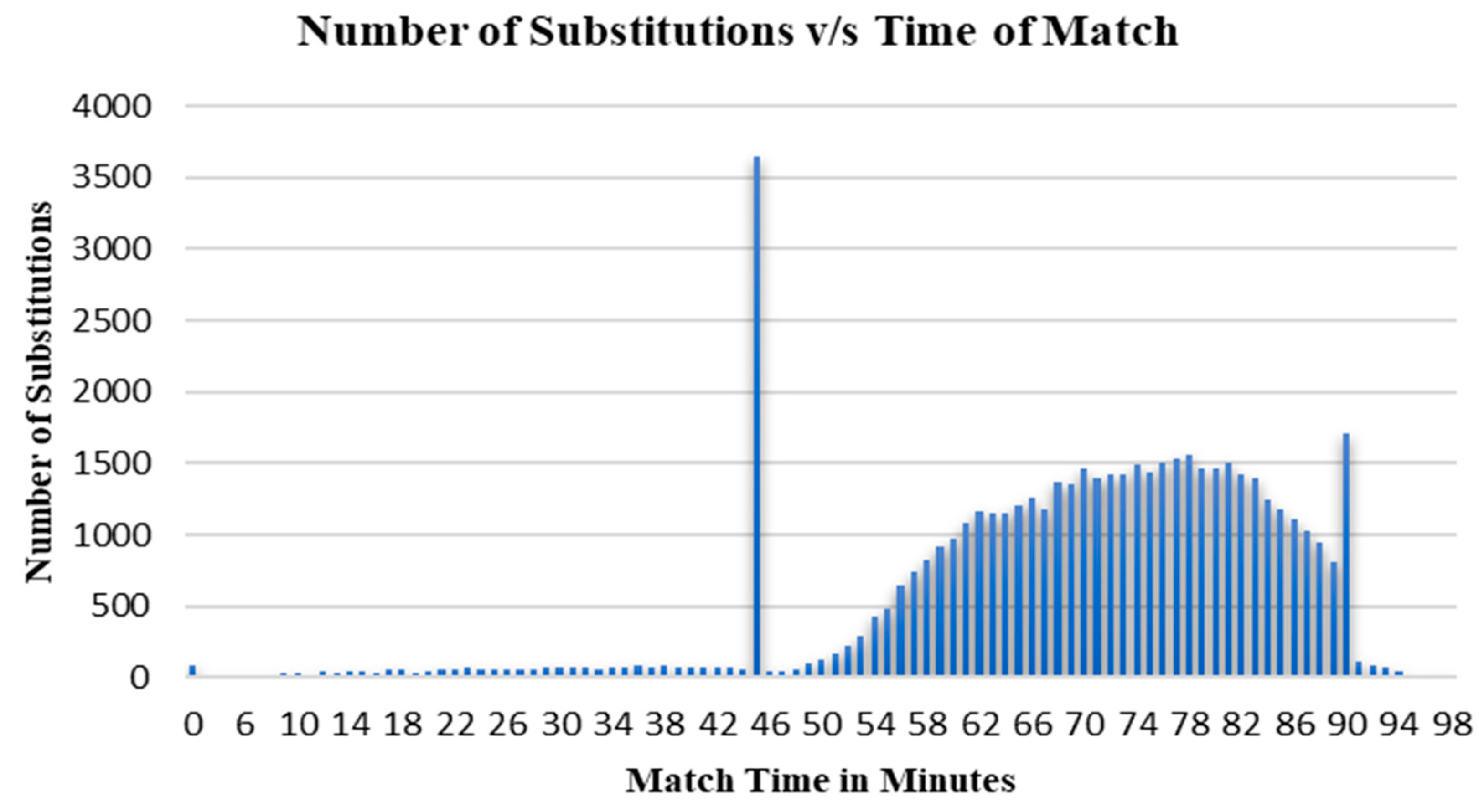
4.2. Analysis of Substitutions Made vs. Time of the Match
An analysis of the substitutions in the German league (
Figure 6) revealed that there were a large number of substitutions that occurred in the first and second halves of the match. Most of the substitutions happened after the 60-min, and many substitutions are observed during the extra/injury time of the second half.
The bulk of the substitutions in the second half shows that those are made based on the current match situation. Further substitutions are being made as the previous substitution may not have caused the desired impact. This can be avoided if the substitutions are predicted correctly. The correlation between the substitutions made in the injury time and the effect of those are not considered in this paper.
4.3. Classifying Substitutions as Positive or Negative
The dataset from Kaggle was loaded into the pandas’ data frame. As discussed in the previous section, a new column called “positive_sub” was added to the dataset to differentiate between positive and negative substitutions based on the goal difference before and after the substitution. If the goal difference improves after substituting a player, the substitution was considered positive. If the goal difference degrades after the substitution, it was marked as a negative substitution. This field ‘positive_sub’ was the value to be predicted by the ML models, based on other parameters. After identifying the positive and negative substitutions and updating the data frame, the graphs of positive substitutions and negative substitutions were plotted against the time of match as shown in the next two sections. An interesting pattern was observed in the positive and negative substitution graphs.
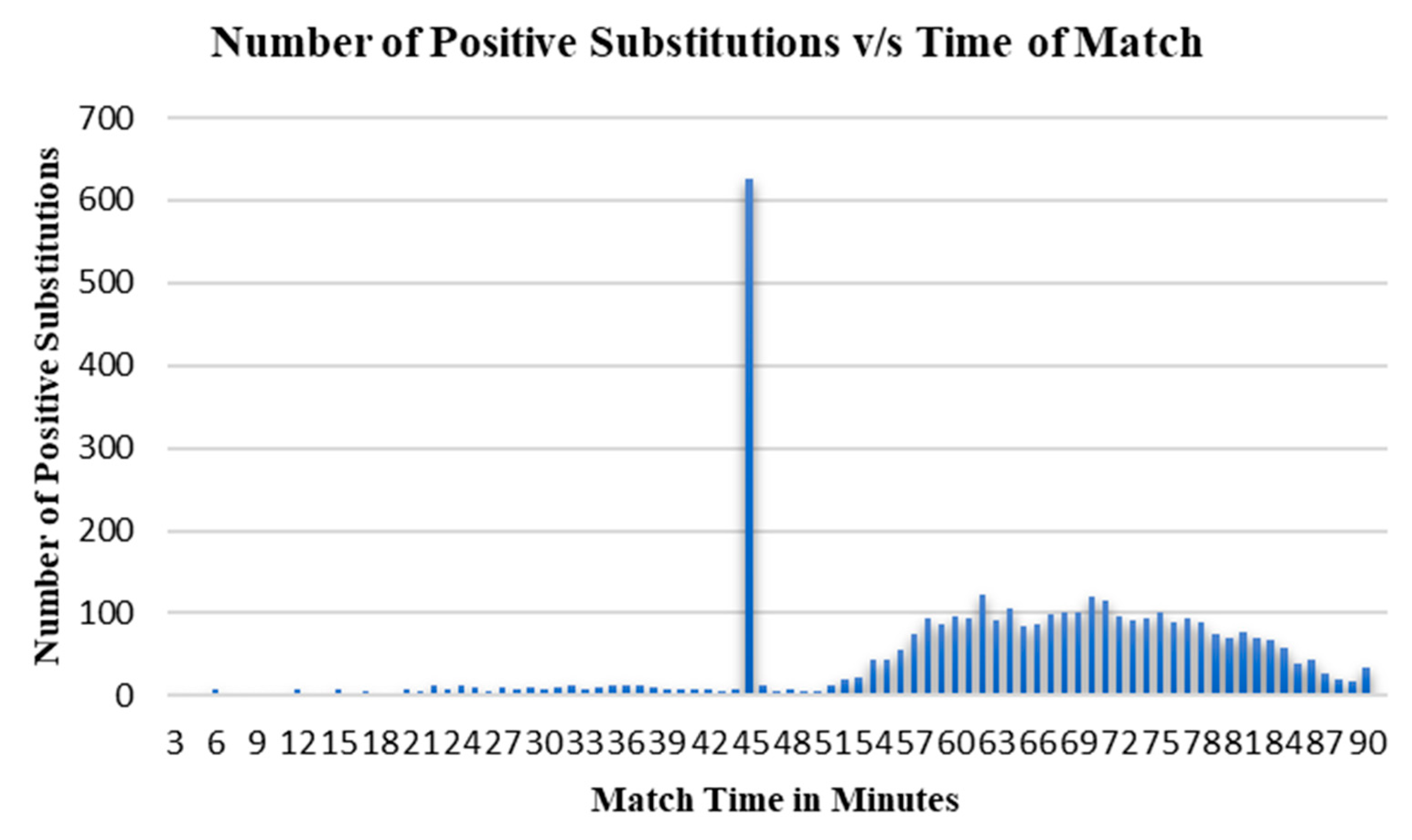
4.4. Substitutions That Resulted in a Positive Impact
It was observed for the positive substitution graph (German league) that the number of substitutions which resulted in a positive impact, reduced as the time left for the match reduces (
Figure 7).
The highest number of positive substitutions occurred at the halftime mark, indicating that teams have time to assess the situation and make the right changes during the break. Substitutions that had a positive effect on the game began to increase from the 60-min mark and decreased after the 75-min mark. This suggests that when players are substituted between the 60-min and 75-min marks, they get enough time to make an impact and thus the team requires fewer substitutions for the rest of the match. As the amount of time left in the match decreases, the effectiveness of the substitutions also decreases.
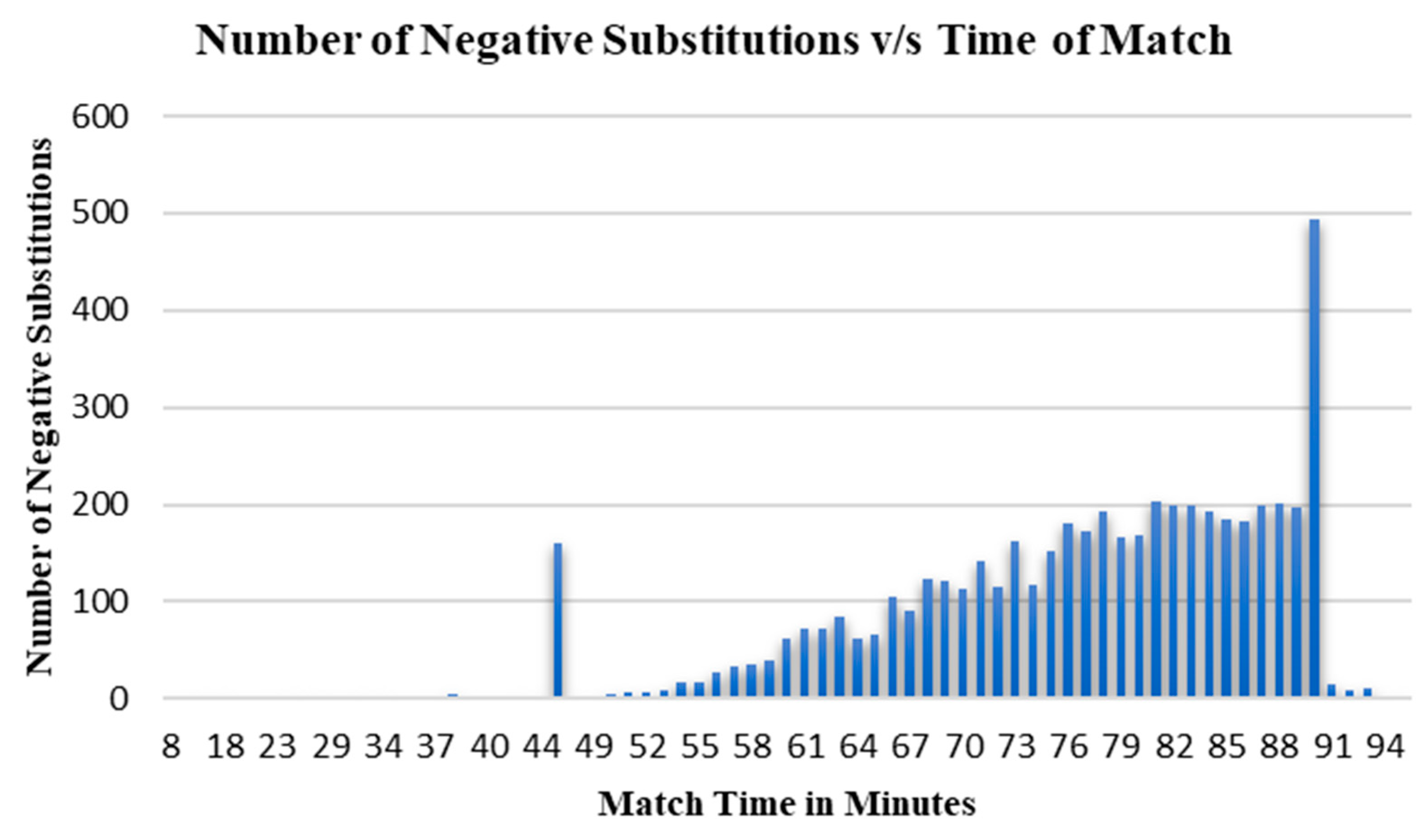
4.5. Substitutions That Resulted in a Negative Impact
For the negative substitution graph (German league) presented in
Figure 8, it was observed that the number of substitutions which resulted in a negative impact, increases as the time left for the match reduces.
The highest number of negative substitutions occurred near the end of the match, with the number increasing linearly from the 60-min mark onward. This implies that the longer the substitution is delayed, the less time the substituted player has to adjust and make an impact, resulting in reduced contributions. As the match time was running out, the coaches tried to make as many substitutions as possible for chances of gaining an advantage, however, often these changes did not make a difference in the score line.
4.6. Analysis of Machine Learning Models on the Dataset
The dataset included data from five European football leagues over seven seasons, consisting of 9074 games and 941,009 events. ML models were developed to predict whether a substitution was positive or negative using the provided input variables. To do this, the dataset was divided into five sets, one for each league (Germany, England, Italy, France, and Spain). Unrelated columns were then removed from the dataset. With the calculated value of the ‘positive_sub’ field in the dataset, the dataset was split into training and testing data and fed into the ML models. The models were trained using 80% of training data and evaluated against 20% of test data.
4.6.1. Analysis of ML Models on German League
The data from the German league (Bundesliga) football was used for all the ML models discussed previously. This dataset included 1608 matches over five seasons (2012 to 2017) with 9136 substitutions. The training data consisted of 7308 substitutions and the test data contained 1828 substitutions.
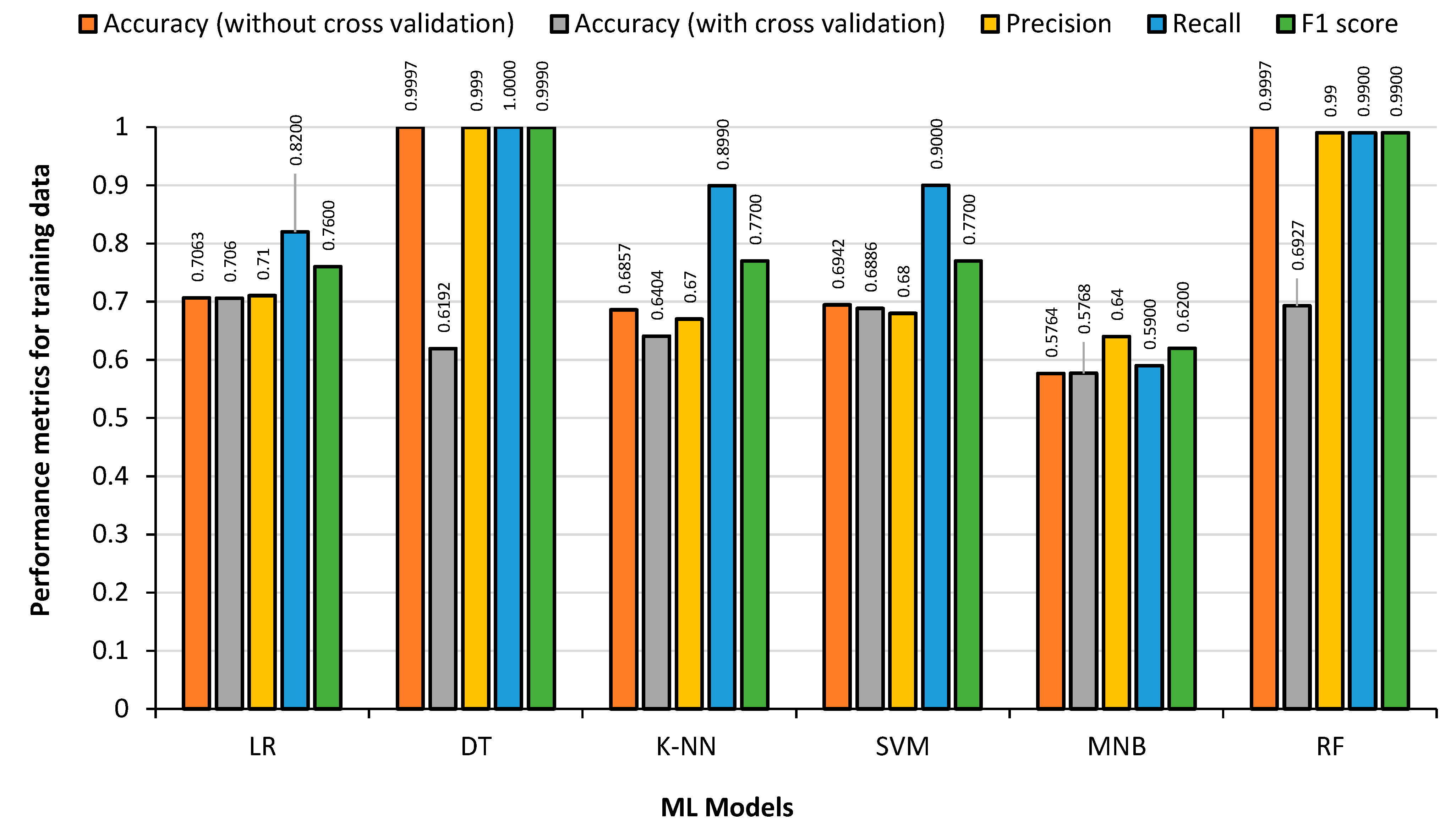
Figure 9 shows the results obtained from the 80% German League training dataset, by feeding the training data back to the generated model to detect the overfitting condition. Cross-validation accuracy, which is obtained by splitting the training dataset into multiple subsets and then using each subset as the test set while using the remaining data as the training set, was calculated along with other parameters using Python sci-kit-learn module. It can be observed that DT and RF classifiers show the highest accuracy, precision, recall and F1 score. RF classifier takes the maximum training time followed by SVM. On the other hand, MNB produces the lowest accuracy as expected, as it is mainly used for text-based identification/classification.
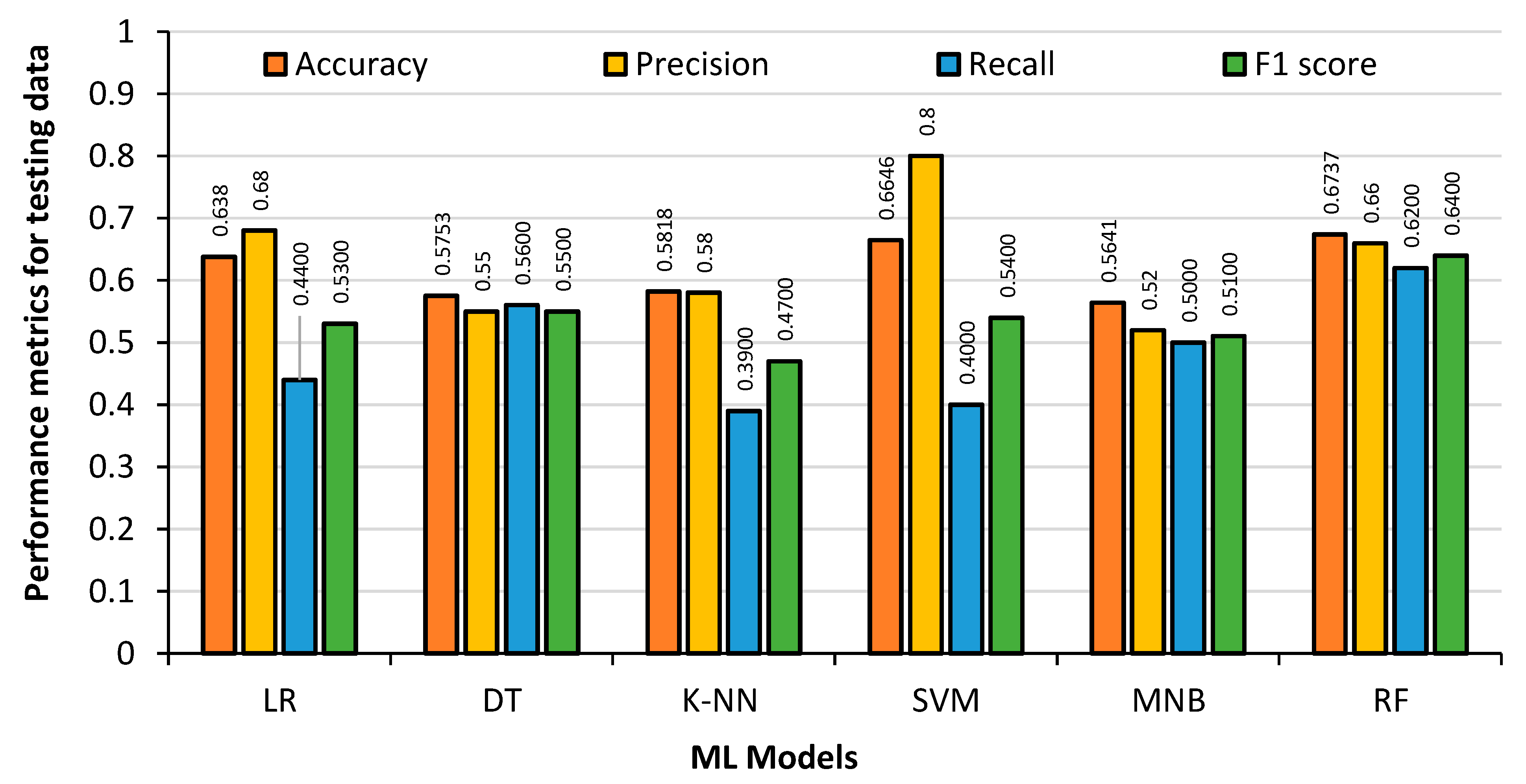
Figure 10 shows the Model results obtained from the 20% German League test dataset. It can be seen that the DT regression Accuracy drops dramatically to 62%. The accuracy of the RF classifier also drops; however, it is not similar to the level of DT regression, owing to the fact that the RF classifier is an ensemble of smaller DT regressions. The accuracy of LR and SVM remains almost the same in the training dataset and test dataset.
Examining the figures above, LR, RF and SVM models obtained the highest accuracy and precision rates for the test data. The DT regression and RF classifier produced the best results with the training data, although it was apparent that they had overfitting problems when tested with the test data. The MNB had the fastest training time and the RF classifier had the slowest. With an accuracy of over 70%, it can be seen that the ML models are accurately predicting player substitutions using the German League dataset.
4.6.2. Analysis of Machine Learning Models in the English Premier League
The data from the English Premier League football was treated the same way as the German Premier League data, and included 1299 matches over five seasons (2012 to 2017) with 7178 substitutions. The training data consisted of 5742 substitutions and the test data contained 1436 substitutions.
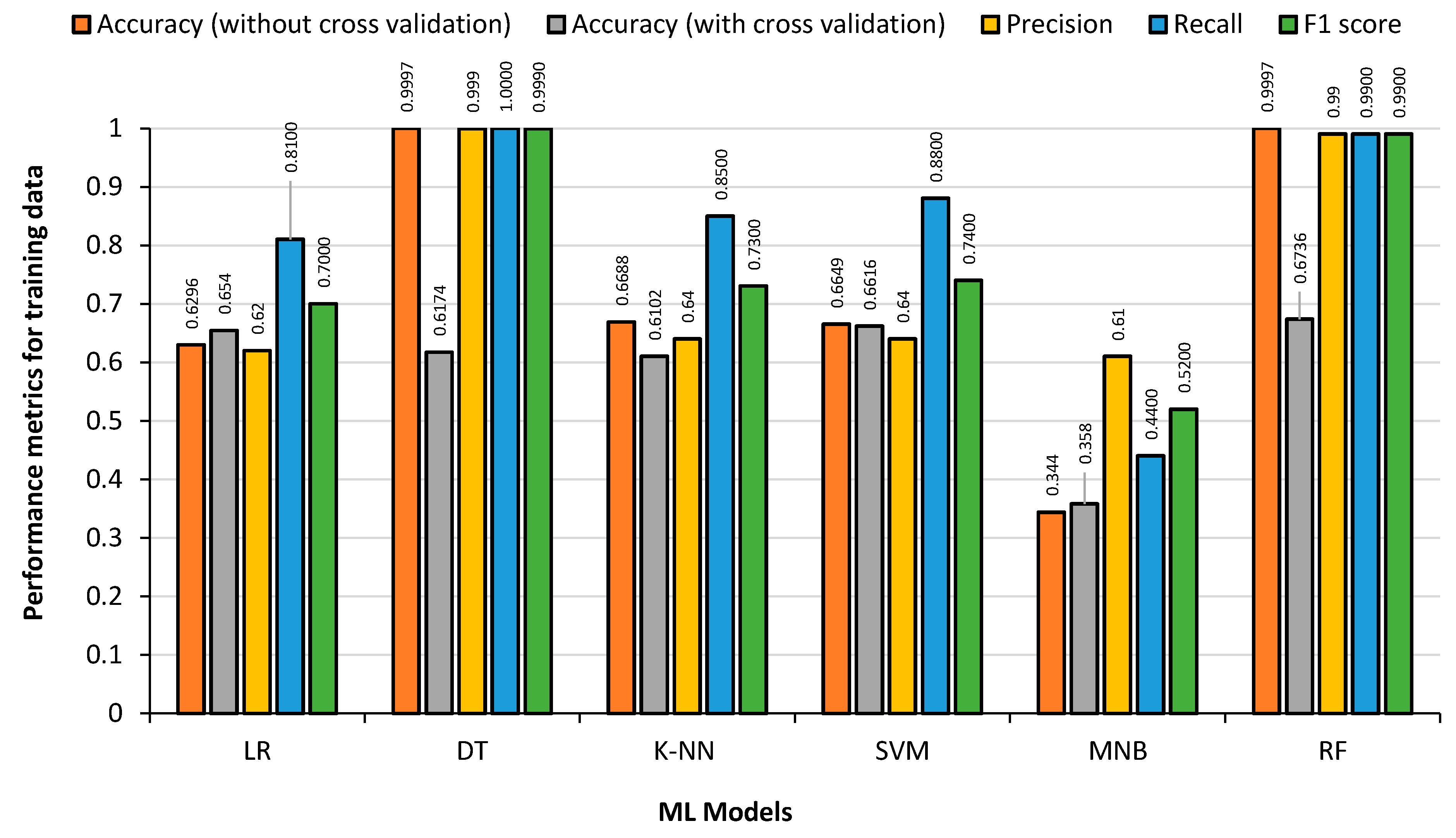
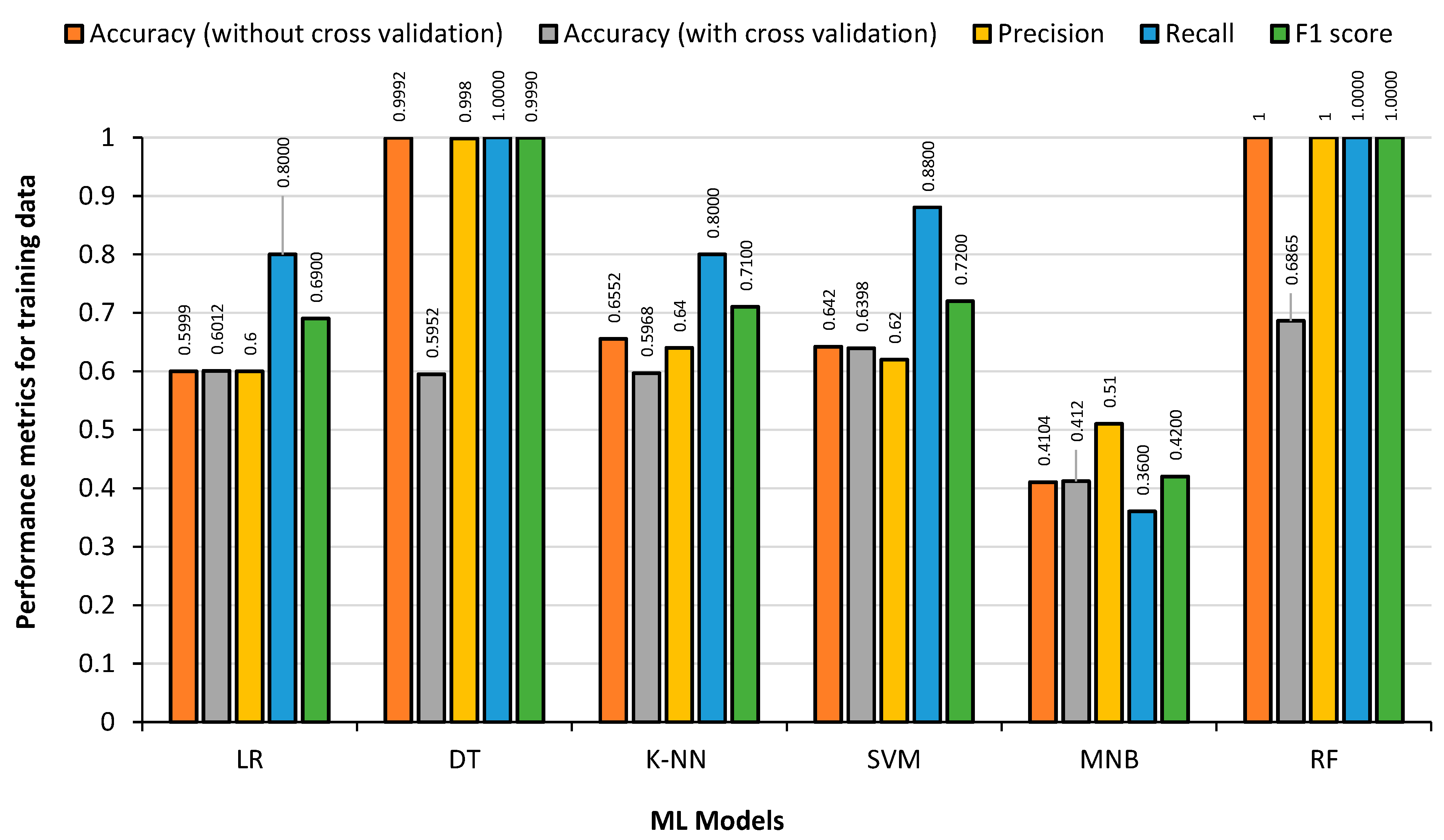
Figure 11 shows the result obtained from the 80% English Premier League training dataset, by feeding the training data back to the generated model to detect the overfitting condition. It is observed that DT regression and RF classifier has the highest accuracy, precision, recall and F1 score. RF classifier takes the maximum training time followed by SVM. MNB has the lowest accuracy as expected, as low as 34%, as it is mainly used for text-based identification/classification. KNN, SVM and LR had almost the same Accuracy and F1 score values.
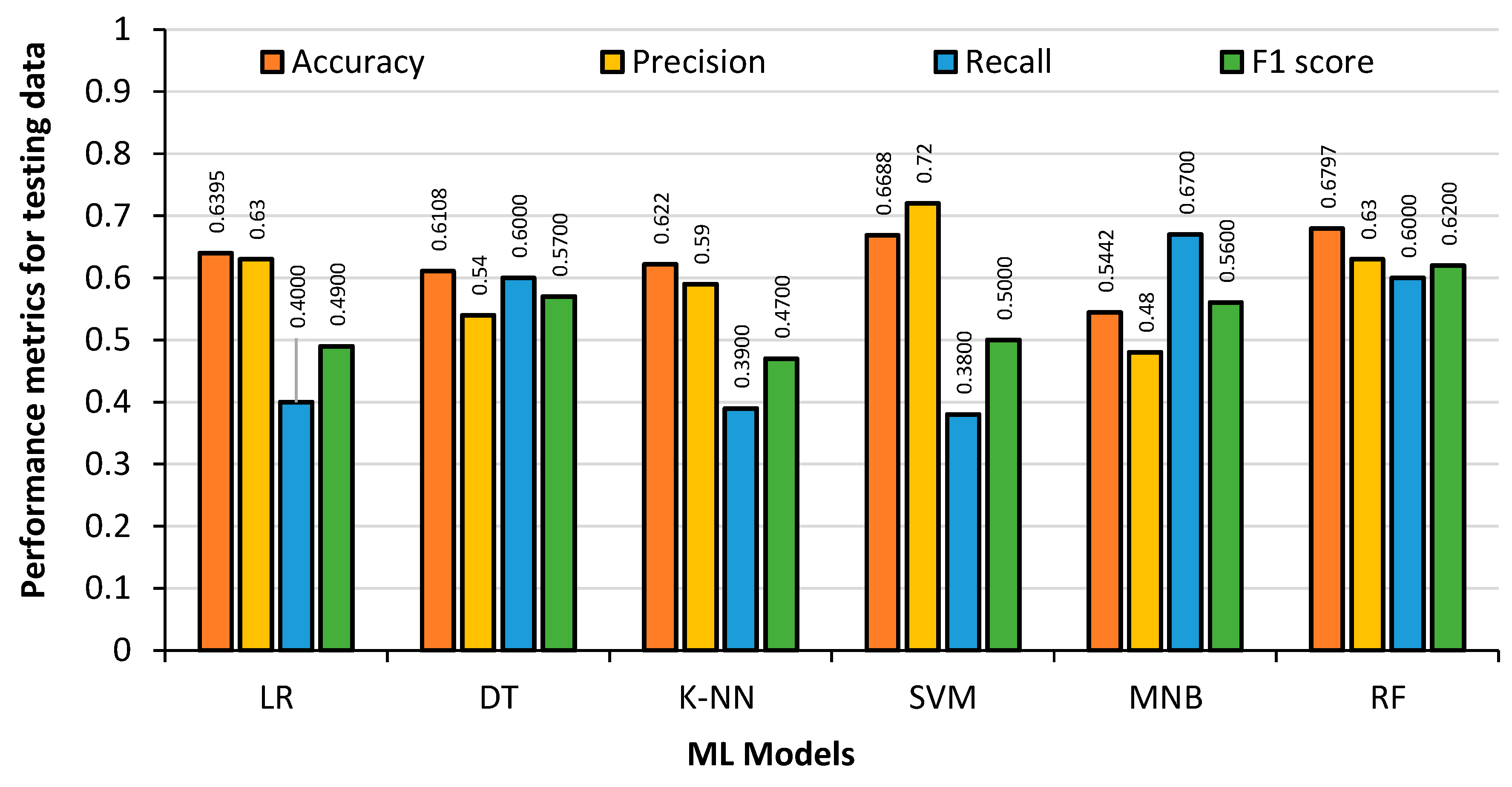
Figure 12 shows the model results obtained from the 20% English Premier League test dataset. It can be seen that the DT regression Accuracy drops dramatically to 61%. The accuracy of the RF classifier also drops to 68%. The accuracy of LR and SVM remains almost the same in the training dataset and test dataset. The accuracy of KNN drops marginally.
Examining the data, it is observed that the RF classifier model had the highest accuracy and F1-score for the test data at 67.97% and 0.62 respectively. The SVM had the highest precision at 0.72. The DT regression and RF classifier results obtained with the training data had overfitting issues, which need to be addressed when selecting the models. The LR had the fastest training time, and the RF classifier had the slowest. With an accuracy of almost 68%, it is clear that the ML models are accurately predicting player substitutions using the English Premier League data.
4.6.3. Analysis of Machine Learning Models on Spanish League
The data from the Spanish League football was treated the same way as the other leagues and included 2015 matches over five seasons (2012 to 2017) with 11,744 substitutions. The training data consisted of 9395 substitutions and the test data contained 2349 substitutions.
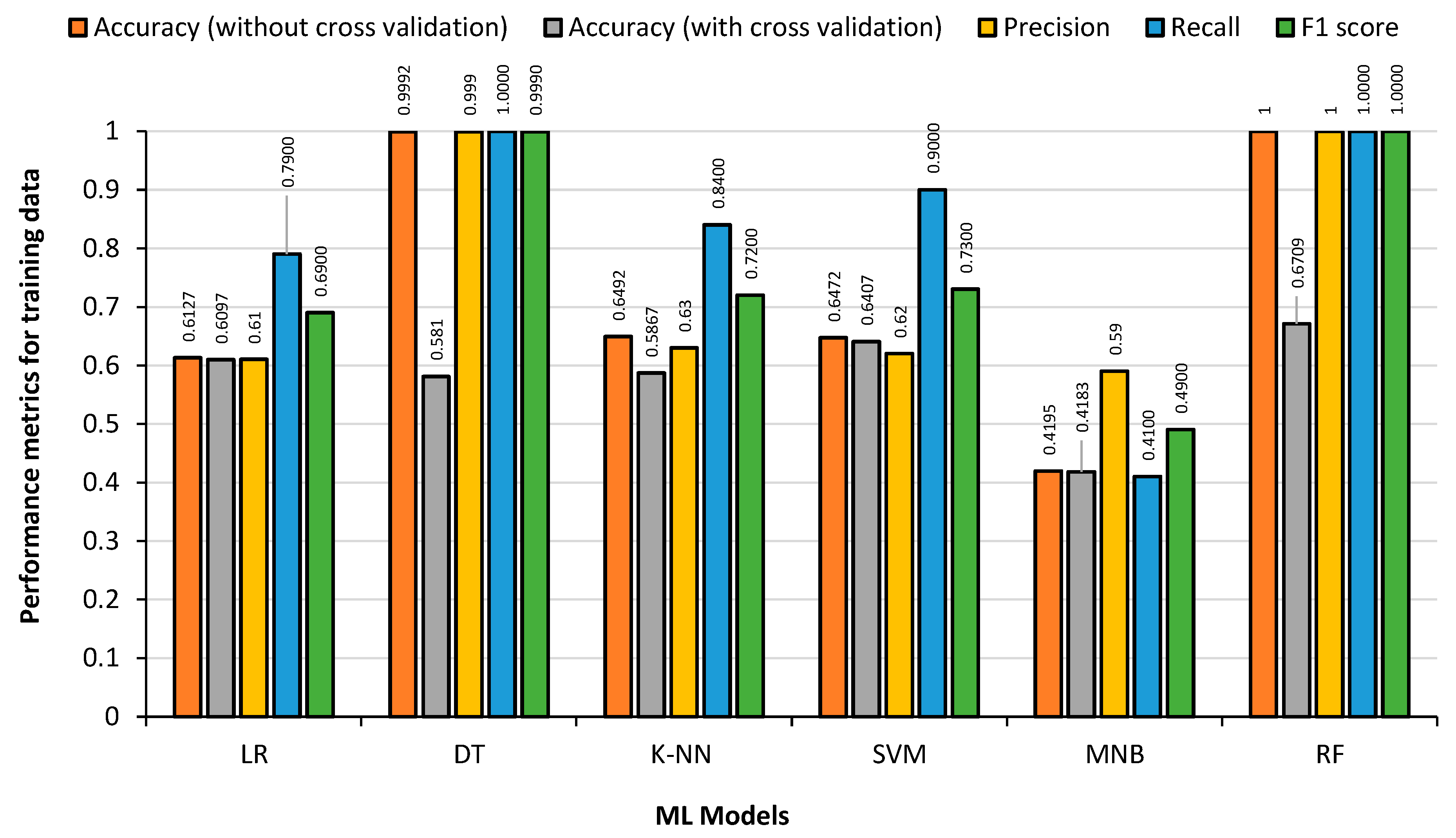
Figure 13 shows the result obtained from the 80% Spanish league training dataset, by feeding the training data back to the generated model to detect the overfitting condition. As seen with the previous league dataset, it can be observed that DT regression and RF classifier has the highest accuracy, precision, recall and F1 score. MNB has the lowest accuracy as with other models. KNN, and SVM had almost the same Accuracy and F1 score values.
The results obtained from the 20% Spanish league test dataset are presented in
Figure 14 where the accuracy of DT regression drops dramatically to 58%. The accuracy of the RF classifier also drops to 68% whereas the accuracy obtained from LR and SVM remains almost the same for the training and test dataset. On the contrary, the accuracy of KNN drops marginally.
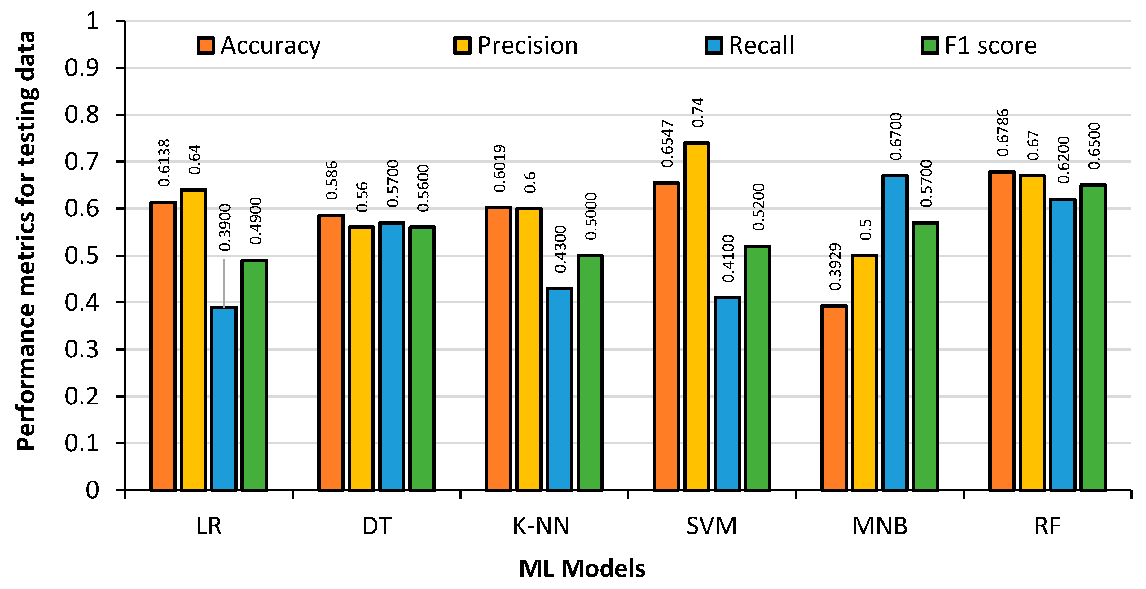
It is observed that the RF classifier model showed the highest accuracy and F1-score at 67.86% and 0.65 respectively whereas the SVM provided the highest precision at 0.67. The DT regression and RF classifier results obtained with the training data had overfitting issues, which need to be addressed when selecting the models. The MNB had the fastest training time, and the RF classifier showed the slowest. By observing the performances, it is concluded that the ML models are accurately predicting the player substitutions with the highest accuracy of almost 68%.
4.6.4. Analysis of Machine Learning Models on French League
The data from the French Football League was treated the same way as the German and English Premier Leagues and included 2076 matches over five seasons (2012 to 2017) with 11,576 substitutions.
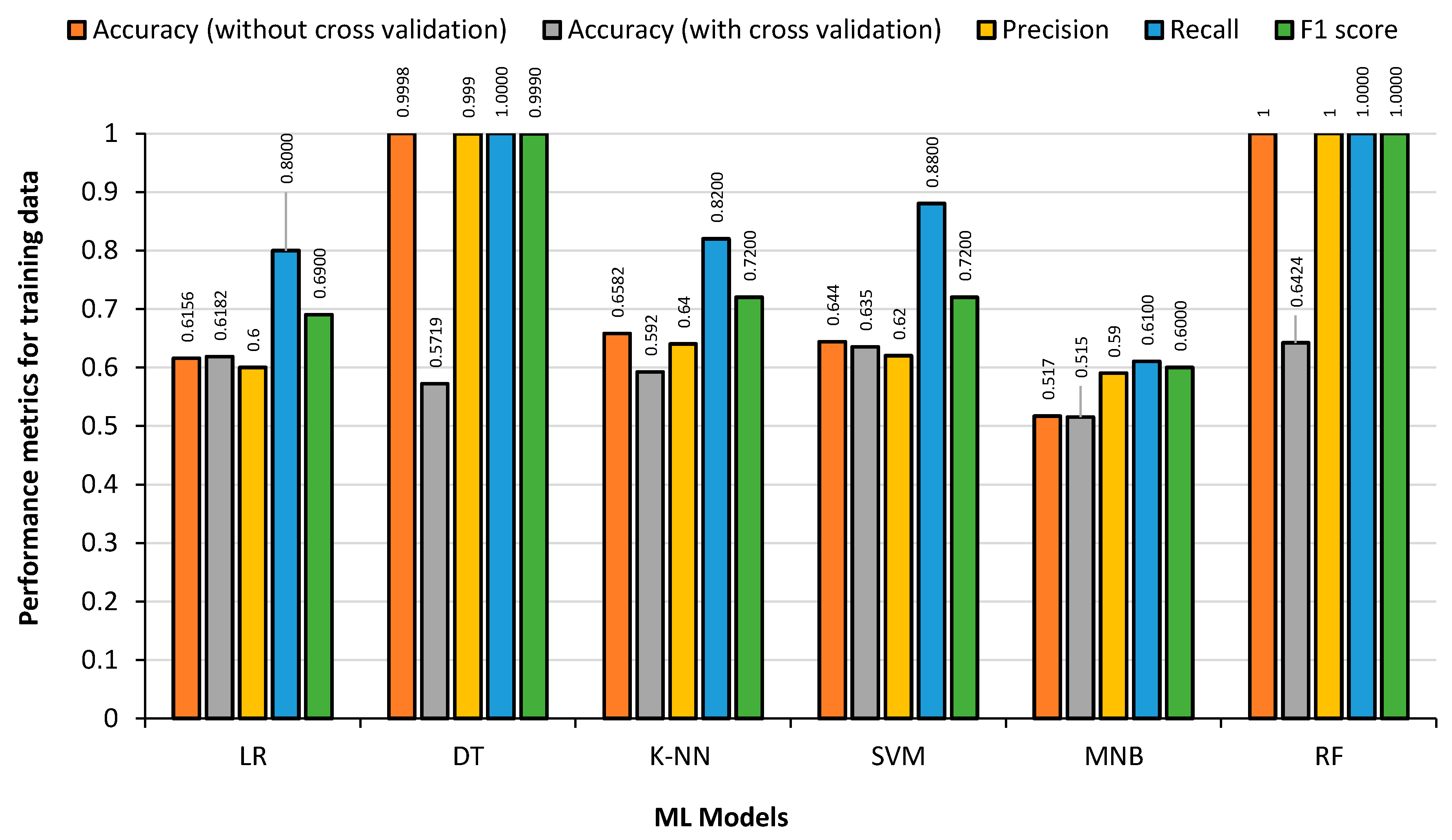
The result obtained from the 80% French league training dataset, by feeding the training data back to the generated model to detect the overfitting condition, is presented in
Figure 15. The training data consisted of 9261 substitutions and the test data contained 2315 substitutions. As seen with the previous league dataset, it can be observed that DT regression and RF classifier has obtained the highest accuracy, precision, recall and F1 score. SVM takes the maximum training time followed by the RF classifier. MNB showed the lowest accuracy as with other models. KNN, and SVM obtained almost the same F1 score values.
Figure 16 shows the model results obtained from the 20% French league test dataset. It can be seen that the DT regression accuracy drops dramatically to 59%. The accuracy of the RF classifier also drops to 68%. Accuracies of LR and SVM remain almost the same for the training and test datasets, while the Accuracy of KNN drops marginally.
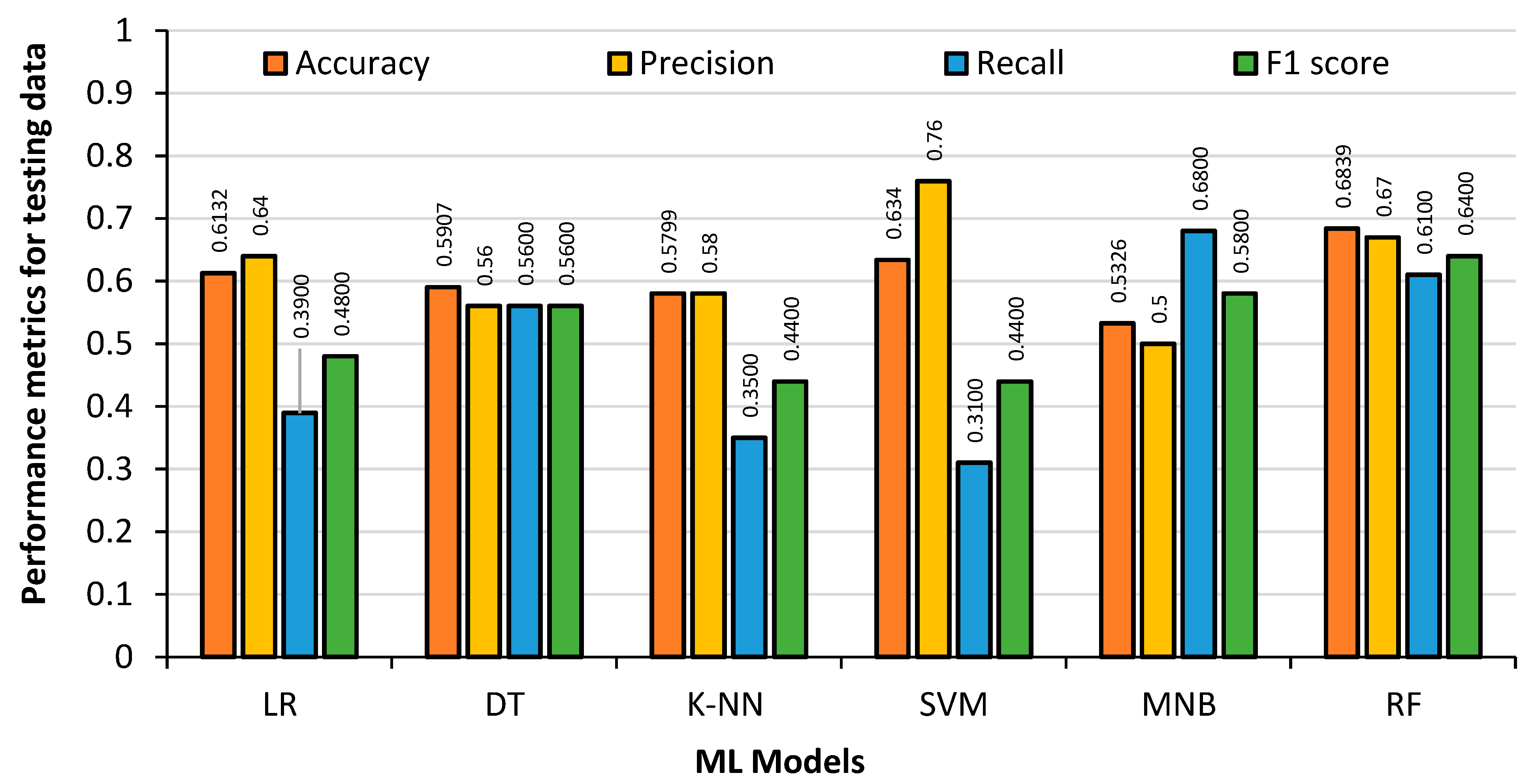
It can be seen that the RF classifier model showed the highest accuracy and F1-score for the test data at 68.39% and 0.64 respectively. The SVM achieved the highest precision at 0.76. The results obtained from the DT regression and RF classifier showed that the training data had overfitting issues, as observed with other football leagues, which need to be addressed during selecting the models. With an accuracy of over 68%), it is seen that the ML models are accurately predicting the player substitutions using the French League dataset.
4.6.5. Analysis of Machine Learning Models on Italian League
The data from the Italian Football League was handled the same way as the other leagues and included 2076 matches over five seasons (2012 to 2017) with 12,104 substitutions. The training data consisted of 9683 substitutions and the test data contained 2421 substitutions.
The result obtained from the 80% Italian league training dataset, by feeding the training data back to the generated model to detect the overfitting condition, has been presented in
Figure 17. The figure showed that DT regression and RF classifier have obtained the highest accuracy, precision, recall and F1 score. MNB showed the lowest accuracy as with other models. KNN, and SVM had almost the same F1 score values. However, LR presented slightly less accuracy value.
Figure 18 revealed the results obtained from the 20% Italian league test dataset where the accuracy obtained by DT regression drops dramatically to 57%. The accuracy obtained by the RF classifier also dropped to 68%. However, the accuracy found from LR and SVM remains almost the same in the training dataset and test dataset, while that achieved by KNN dropped marginally. RF classifier model had the highest accuracy and F1-score for the test data at 67.37% and 0.64 respectively. The LR showed the highest precision at 0.68. In addition, the results obtained by DT regression and RF classifier with the training data had overfitting issues, which need to be addressed when selecting the models.
An RF classifier consists of a large number of decision trees, and each tree must be trained and evaluated. As our datasets were huge, it resulted in more trees in the RF, however, it provided the best prediction of the player substitutions effectively with an accuracy of over 67% and was able to handle large and complex datasets.
4.7. Machine Learning Model Result Analysis
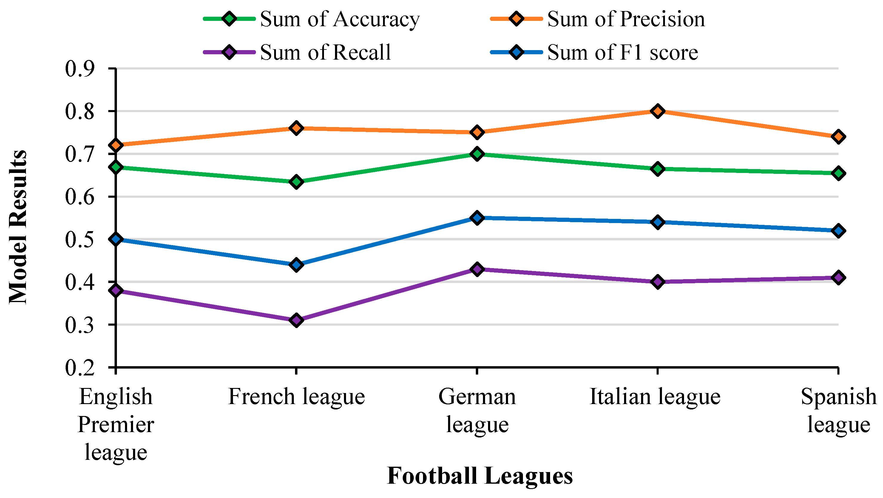
4.7.1. Logistic Regression (LR)
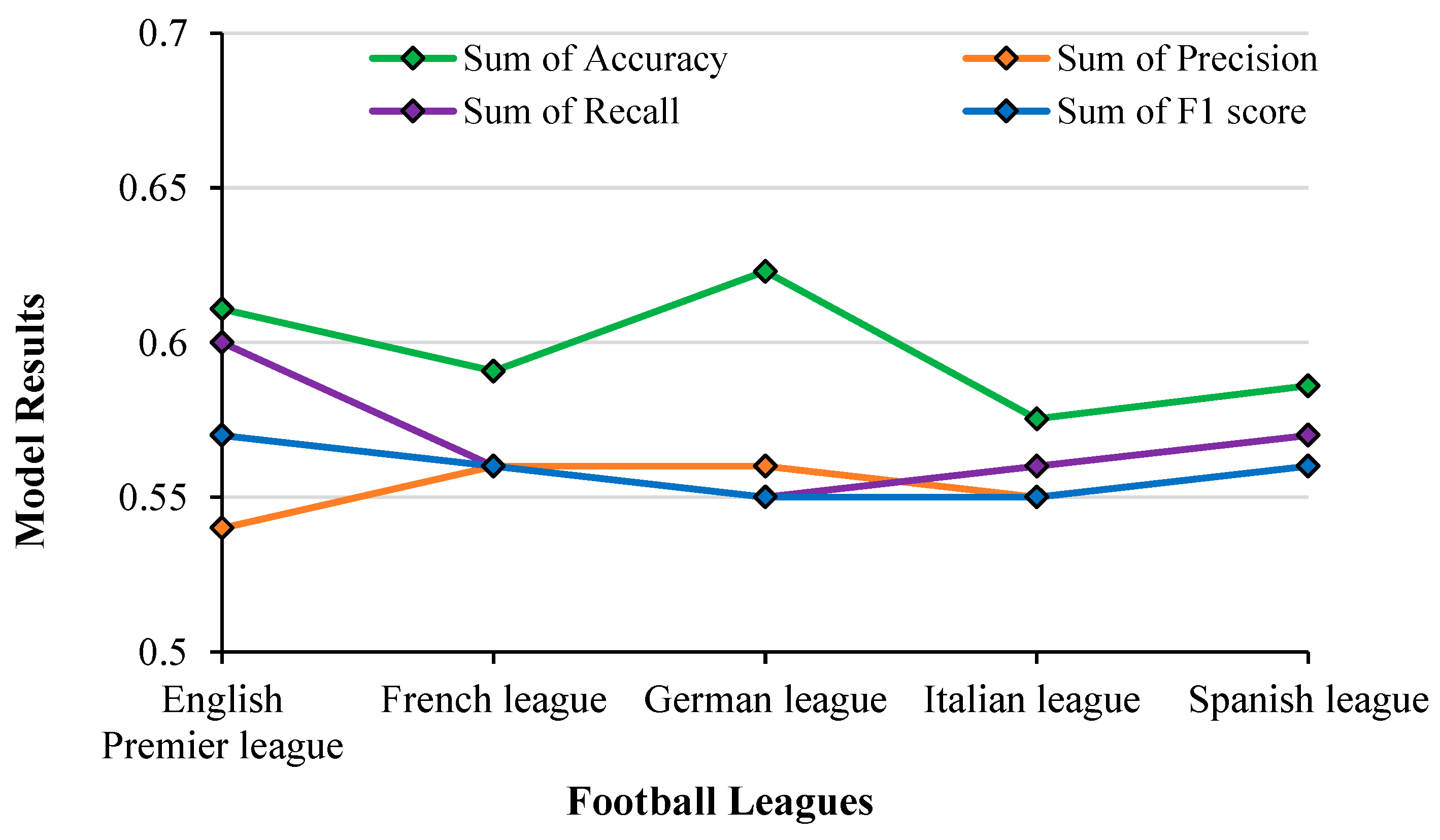
The prediction outcomes obtained from an LR model on test data across numerous football leagues are presented in
Figure 19. Following Equation (1), reveals that feeding the test data into the linear regression hypothesis function resulted in a maximum accuracy of approximately 70%.
The accuracy of LR varied between 60% and 70% across all the leagues. Precision values remained almost flat between 0.63 and 0.68 across all leagues. The F1-score and Recall almost followed the same pattern with higher values for the German league and relatively less values for the other leagues. Except for the German league, both the F1-score and recall for LR stayed within a delta of 0.05 across all leagues. As per the definition of the F1 score (harmonic mean of precision and recall), from the graph, it is seen that the plot of the F1 score clearly lies between the plots of Precision and Recall. It is also seen that the plot for accuracy aligns in proportion to the F1 score where the Accuracy and F1 score follow the same pattern. For example, in the German league, they are both high, where the LR model provided correct predictions with a high degree of precision. In summary, as accuracy and F1 score followed the same pattern and obtained better results, the model’s performance is consistent across both metrics.
4.7.2. Decision Tree Regression
The results achieved by applying DT regression to test data across multiple football leagues are presented in
Figure 20. The accuracy obtained by DT regression varied between 56% and 62% across all the leagues. Precision, Recall and F1-Score values remained almost flat across all leagues between 0.55 and 0.57 except for the English Premier League, where Recall was at 0.6 and Precision at 0.54. The accuracy aligns in proportion to the F1 score for Italian French, Spanish and English leagues, indicating that the DT model is showing a large number of correct predictions with a high degree of precision. As accuracy and F1 score followed the same pattern, the model’s performance is consistent across both metrics and the model performed well on both accuracy and F1 score. However, in the case of the German league, the Accuracy and F1 score do not seem to be aligning and hence it can be concluded that the model is making a smaller number of correct predictions, when compared to the other leagues.
4.7.3. K-Nearest Neighbor Regression
The outcomes of KNN model on test data across various football leagues have been presented in
Figure 21. As defined in Equation (2), the KNN uses Euclidean distance to identify similarities between new data and existing data, thereby allowing the input to be classified into the most similar category. When the test data was input into the model, an accuracy of nearly 65% was achieved.
It was observed that the accuracy varied between 58% and 66% across all the leagues archived by the KNN. Precision values followed a similar pattern with Accuracy. Recall and F1-Score almost followed the same pattern with higher values for the Spanish league and relatively lower values for other leagues. Both F1-score and Recall for K-NN regression stayed within a delta of 0.1 across all leagues.
It is also seen that the Accuracy and Precision values are almost identical in all the datasets. This observation indicates that the KNN model’s performance on the test data is consistently accurate and precise, showing that the KNN model is capable of correctly classifying and predicting the substitution based on the inputs consistently, with a high degree of accuracy and precision.
4.7.4. Support Vector Machine
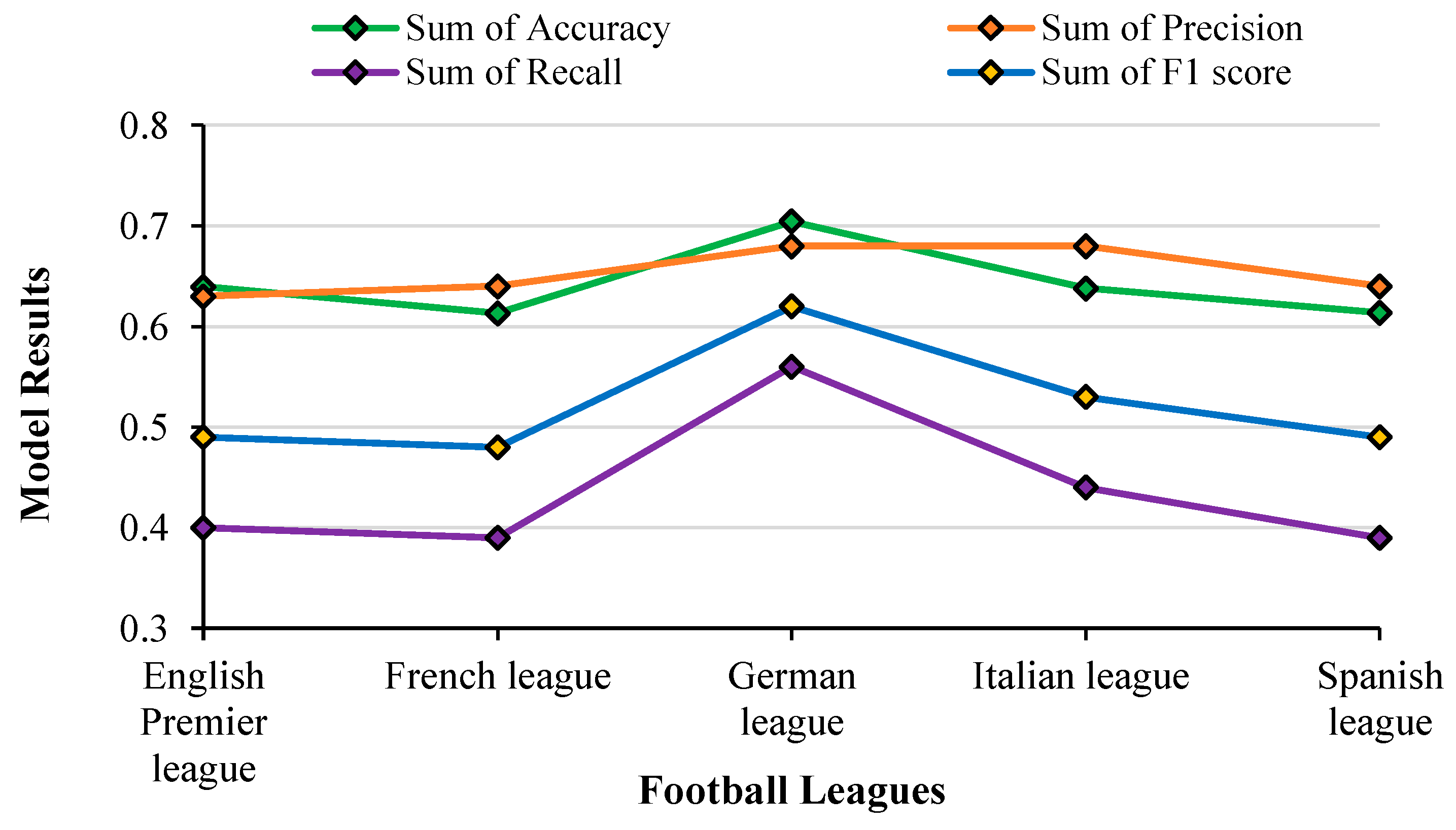
Figure 22 shows the results obtained by SVM on test data across numerous football leagues. The SVM maps the training data points to locations in space, maximizing the distance between them. An accuracy of approximately 70% was achieved when the test data was fed into the model.
It was observed that the accuracy varied between 63% and 70% across all the leagues with the highest for the German league after analysing the results of SVM. Precision values stayed between 0.7 and 0.8 with the highest value for the Italian league. Recall and F1-Score almost followed the same pattern with higher values for the German league and lowest for the French league. It is clear that for SVM, the Precision value is tightly correlated with the size of the dataset. For the dataset with the highest number of entries (Italian), the precision value is maximum, which is followed by Spanish, French, German and English (the dataset with the least number of entries). The plot of the F1 score clearly lies between the plots of Precision and Recall (as it is the harmonic mean of them).
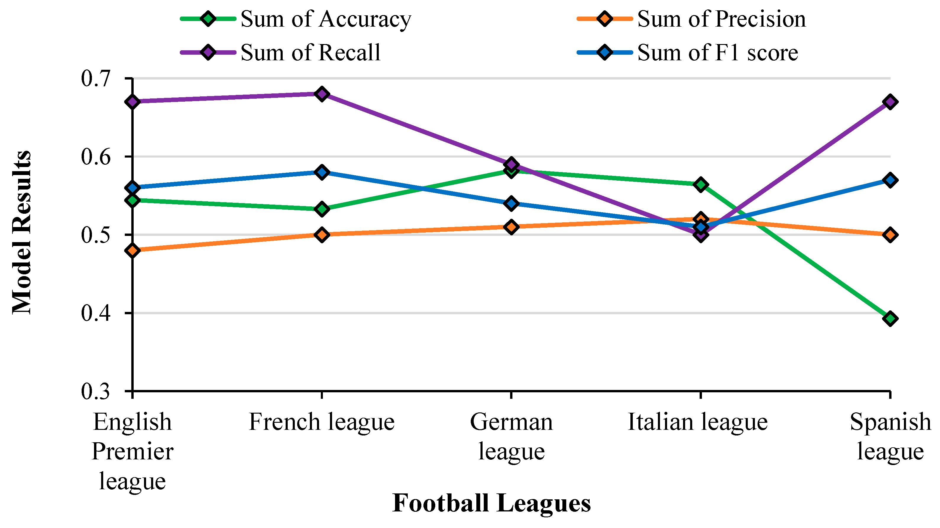
4.7.5. Multinomial Naïve Bayes (MNB)
The outcomes of using an MNB ML model on test data across numerous football leagues are presented in
Figure 23. In the MNB algorithm, predictions are based on tags, and thus the expected accuracy of the model in this scenario is lower.
The results of test data for MNB were analyzed and observed that the accuracy remained at the same levels (~55%) for all leagues except the Spanish league, where the accuracy dipped to 40%. Precision and F1-score remained almost identical. The recall value was lowest for the Italian league at 0.5 and highest for the French league at 0.68. It is difficult to arrive at a solid result due to the deviations except for the Italian league. This was almost expected as MNB is normally used only in text processing and not in variable classification. For the Italian league, the Accuracy, and F1 scores match each other which indicates that the model’s performance is consistent across both metrics.
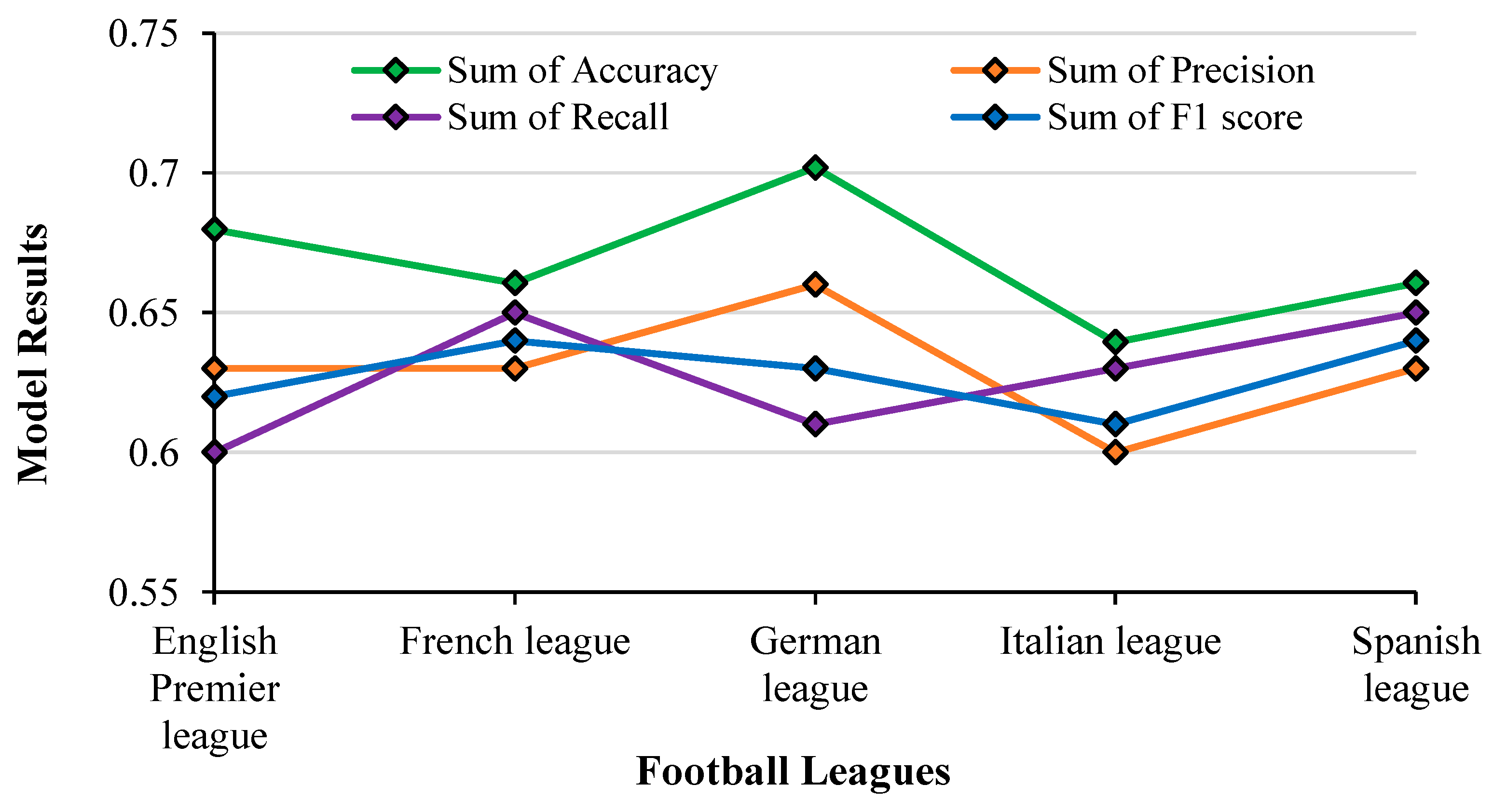
4.7.6. Random Forest Classifier
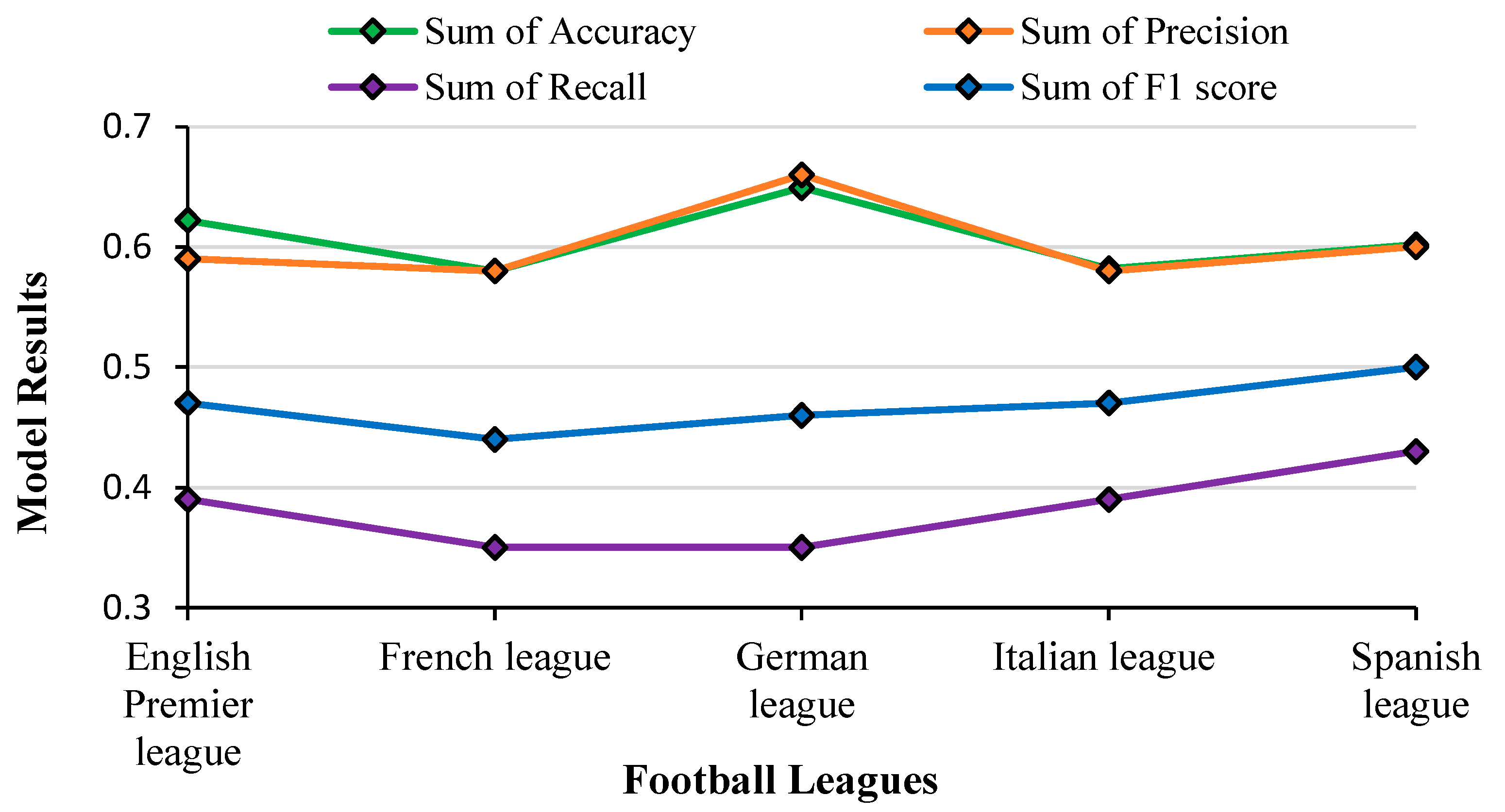
In this subsection, the outcomes obtained by the RF classifier on test data across numerous football leagues (
Figure 24). The dataset was broken up into numerous small decision trees, creating an ensemble that provided more accurate predictions when compared to the DT algorithm.
Based on the results of MNB, it was observed that the distribution of Accuracy, Precision and F1-Score values followed almost the same pattern. The highest accuracy was for the German league at 70% and the lowest was for the Italian league at 64%. Recall values varied between 0.6 to 0.65 across all leagues.
The results of the RF classifier model showed the best relationship between Accuracy, F1 score, Precision and Recall across almost all leagues, which represents that the model’s performance on the training or validation data is better and consistent across these different evaluation metrics. This also shows that the RF Classifier model demonstrates a large number of correct predictions with a high degree of precision.
4.7.7. Comparison of Model Training and Total Times across All Leagues
The summary of training time taken for each ML model across all 5 leagues is presented in
Figure 25. Italian league having 12,104 substitutions clearly has the highest training time followed by the Spanish league (11,744), the French league (11,576), the German league (9136) and English Premier League (7178). It is clear from the figure that model training time taken by SVM and RF classifier increases drastically as the elements in the input dataset increase.
The total time taken was worst for RF Classifier in the Italian league, where it went up to 9 s. MNB had the best total training time across all leagues. It took just 0.23 s to train all datasets. The training time increases as the size of the dataset increases.
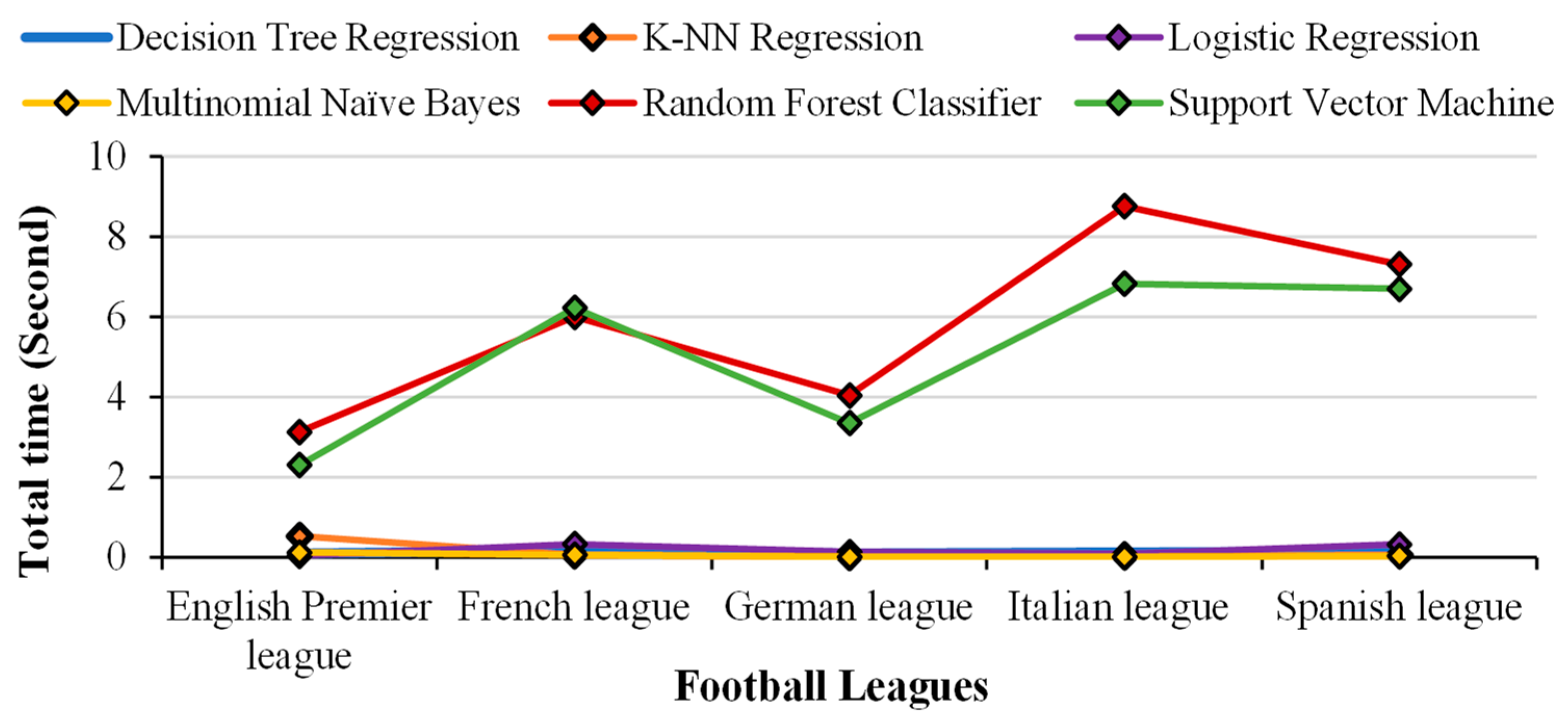
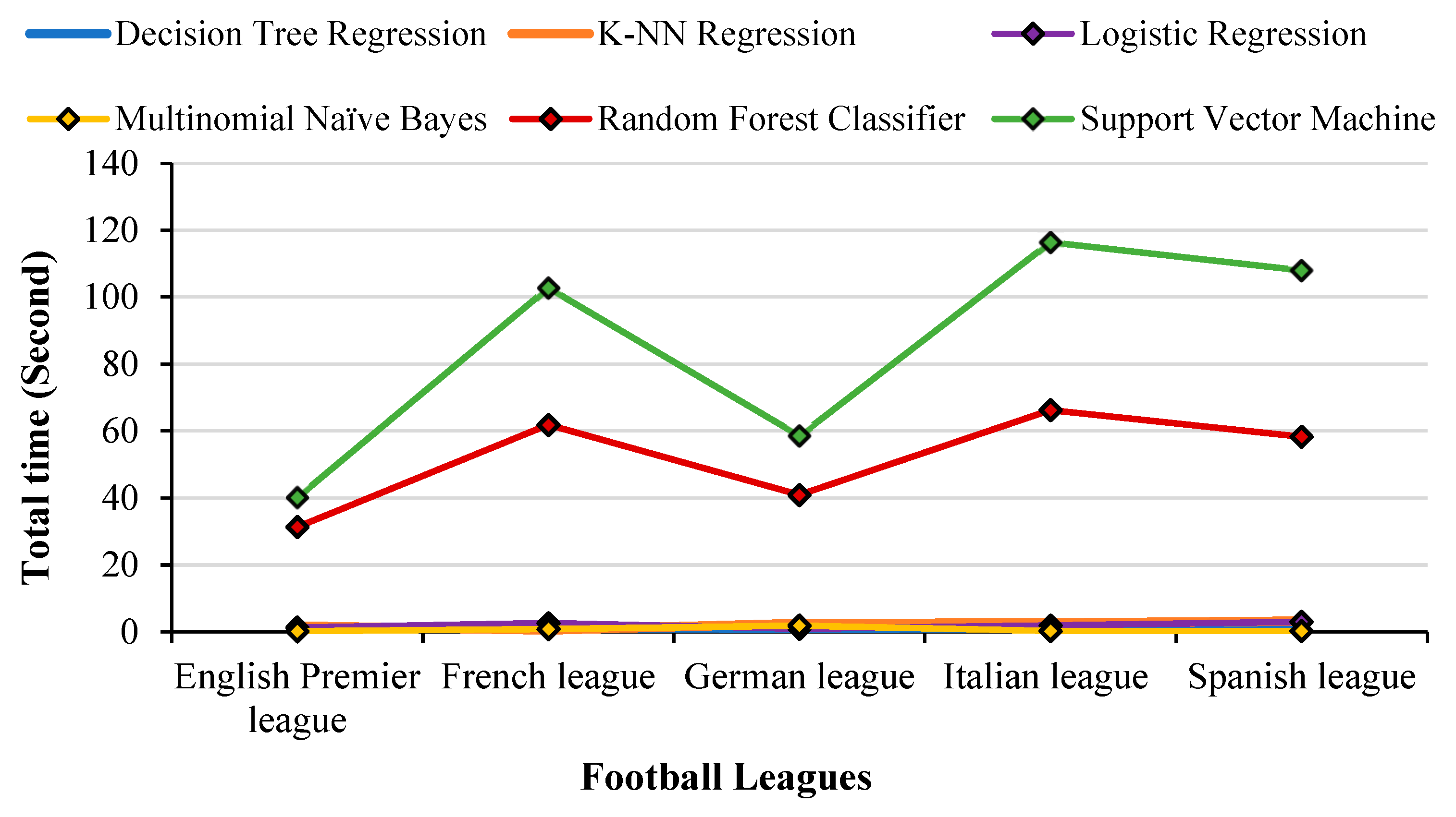
The comparison of the total time taken (including training, testing, model fitting, and confusion matrix generation) for all the ML Models across all 5 leagues (
Figure 26).
As the elements in the input dataset increase, the total time taken also increases by the SVM and RF classifier. The total time taken found was worst for SVM in the Italian league, where it took up to 2 min for the entire process to complete. MNB took less total time which was just 3.3 s to calculate values for all the leagues. It is also seen that the total time including training, testing and formatting time increases due to increasing the size of the dataset.
4.8. Critical Analysis and Discussion
4.8.1. Strength of This Research
It is definite that the use of ML and AI algorithms can remarkably help football teams and managers in various aspects (e.g., prediction of substitution). This proposed work provides a study of substitution data by analyzing over 50 thousand substitutions and programmatically categorizing them as positive or negative based on how the match scoreline changed before and after substitution.
This work showed a comparison study between various regression and classification algorithms and provides an option to choose the best one based on performance, complexity, or accuracy. Achieving over 70% accuracy on all the football leagues in this work, paved an ideal platform for anyone who would like to use the huge amount of substitution data to implement in live matches.
The dataset was structured with a huge number of events, almost a million. This was categorized, filtered and cleansed for our use, by programmatically extracting substitution events, which were around 51 thousand in total (5% of the total events). The goal-scoring details were also filtered out with timestamp details to programmatically determine substitution advantage. This data can now be used as a base to perform any further study or analysis [
43].
4.8.2. Limitation
This research work comes up with various ML algorithm results based on historical substitution data. As a result, this prediction results will not be favorable for a new football player, as the player’s historical substitution data will not be available for comparison. This may be overcome by collecting data from the old matches played by the new player and merging it with the current dataset.
The developed model currently does not consider the playing position of the player substituted. Based on playing position, if a defender is substituted, substitution can be marked positive if accepted goals remain the same. If a forward player is substituted, substitution can be marked positive if the goals scored increase. Thus, the accuracy can be improved further.
Player names may be misspelled or updated in different formats in the dataset at different instances, which has not been considered for this research work. Cleansing methods can be implemented to merge misspelled names and if done properly accuracy can be improved accordingly.
Goal-keeper substitution needs to be handled separately by considering on-field penalties and penalty shoot-out data which has not been considered in this proposed work. As goal-keeper substitutions are very minimal and shoot-outs are very minimal in European league matches, therefore, the relevant data was ignored for this proposed work. The relatively low accuracy of 70% is attributed to the fact that some of the models were overfitting the data during training, which resulted in reduced accuracy with the test data. The dataset also needs to be cleaned as per the points mentioned in this section, to enhance the prediction accuracy of player substitution.
In this paper, the aim was to measure accurately the prediction performance of player substitution across various ML models. However, the results from different models were not merged/unified to propose an optimal solution.
Furthermore, the model could not be compared with the literature as this type of result has not been reported before.
4.8.3. Scope for Future Work
In this research, the strength of the team and different team composition is not considered while classifying the impact of substitution. This can be added as a descriptor based on the current point table standing and previous season team standings of both playing teams. Adding this descriptor may provide accurate results and can be considered for future work. The relevance of each descriptor used for training the ML model is not considered in this research. By considering the relevance, the model training time can be significantly reduced. For example, by training the model without including a dataset from a specific team and then testing the model with data from the excluded team, the relevance of the ‘team’ descriptor can be signified. A study could be conducted to see which descriptor has more relevance. A player’s team name may have less significance compared to the opponent’s team name or vice versa. This can be obtained by excluding/adding descriptors while training the ML model.
The possibility of correlation among training and testing datasets is not considered in this paper. There may be a correlation between training data, created with the data from a set of teams, and with the test data, tested on data from another team. This can be considered as future work.
This paper analyses multiple machine learning models and provides a comparative study of accuracy, precision, performance, etc. Integrating the results from all the models and coming up with a unified optimal solution can be considered for future work.
5. Conclusions
Data analytics and ML algorithms are gaining widespread attention in the sports world, where football is no exception. Substitutions in football offer team managers the opportunity to alter team composition and strategy while the game is in progress. Data analytics and forecasting can be incredibly helpful in determining the best substitute player who can provide a game advantage, if substituted at the right time. This can be achieved by employing data classification and regression techniques to historical substitution data from past matches. This research work proposed a novel approach to effectively integrate ML algorithms into live football matches in order to place timely substitutions to achieve game advantage and potentially alter the outcome of the match.
In this research work, an intelligent system was developed for predicting substitutions with high accuracy and minimal complexity by combining features extracted via LR, SVMs, RF, MNB, KNN, and DT. Over 51,738 substitutions from 9074 European league matches were entered into the system, created using Python and ML models, to predict the best possible substitution that could result in the greatest game advantage. The proposed system achieved a high accuracy (70%) with RF Classifier yielding the best accuracy on the test data, and SVM providing the highest precision data. This work provides a baseline and strong starting point for any future investigations in this domain. By addressing the constraints outlined in the previous section, the system can be strengthened further by accommodating the above-mentioned factors in the previous subsection. The proposed techniques will facilitate the use of ML algorithms in sports and will pave making accurate decisions during live football matches.


