Article

A Space-Time Framework for Sentiment Scope Analysis in Social Media

Department of Information Engineering (DII), Polytechnic University of Marche, Via Brecce Bianche 12, 60121 Ancona, Italy
*
Author to whom correspondence should be addressed.
Big Data Cogn. Comput. 2022, 6(4), 130; https://doi.org/10.3390/bdcc6040130
Submission received: 3 October 2022 / Revised: 28 October 2022 / Accepted: 31 October 2022 / Published: 3 November 2022

Abstract

:
The concept of scope was introduced in Social Network Analysis to assess the authoritativeness and convincing ability of a user toward other users on one or more social platforms. It has been studied in the past in some specific contexts, for example to assess the ability of a user to spread information on Twitter. In this paper, we propose a new investigation on scope, as we want to assess the scope of the sentiment of a user on a topic. We also propose a multi-dimensional definition of scope. In fact, besides the traditional spatial scope, we introduce the temporal one, which has never been addressed in the literature, and propose a model that allows the concept of scope to be extended to further dimensions in the future. Furthermore, we propose an approach and a related set of parameters for measuring the scope of the sentiment of a user on a topic in a social network. Finally, we illustrate the results of an experimental campaign we conducted to evaluate the proposed framework on a dataset derived from Reddit. The main novelties of this paper are: (i) a multi-dimensional view of scope; (ii) the introduction of the concept of sentiment scope; (iii) the definition of a general framework capable of analyzing the sentiment scope related to any subject on any social network.

1. Introduction

Suppose we are at the shore of a lake on a becalmed day with a flat lake surface. Suppose now that we throw a stone into it. We can see how, starting from the point where the stone falls, the water begins to ripple, and small waves are created. These waves are higher near the point where the stone fell while they become smaller and smaller as we move away from it, until they disappear. The heavier the stone thrown, the higher the waves and the farther they propagate. As time passes, the height of the waves tends to decrease until, if no more stones are thrown into the lake, they disappear and the lake surface becomes motionless again. In our opinion, this image describes better than any other what is meant by “scope”. From a more formal point of view, in the Concise Oxford Dictionary (Concise Oxford Dictionary—https://en.oxforddictionaries.com (accessed on 15 September 2022)), scope is defined as “the extent of the area or subject matter that something deals with or to which it is relevant”.
Certainly, there are several similarities between the concept of scope and some other ones used in sociology. Consider, for example, the concepts of centrality, reliability, power, reputation, influence, trust, diffusion, etc. In fact, scope goes beyond these concepts and, at the same time, embraces all of them. In fact, they can be seen as different aspects of scope, which certainly exert their influence on it.
Scope has already been studied in past literature. For example, Ref. [1] analyzed the scope of users and hashtags in Twitter, while [2] proposed an approach to compute the scope of a smart object in a Multi-IoT context. In Refs. [3,4,5,6,7,8], the authors presented approaches to analyze some aspects of scope (e.g., reliability, trust, and influence) for users and/or hashtags. In Ref. [9], the authors studied the distribution of the influence of a user across the network, while in Ref. [10], the authors analyzed the attractiveness of users in networks.
In the social network context, which we focus on in this paper, another much analyzed concept is that of user sentiment. Sentiment analysis is one of the most active research strands regarding social networks and, more generally, artificial Intelligence and data analysis [11,12,13,14]. In fact, nowadays, millions and millions of people express their sentiments on the most disparate topics through social networks [15,16,17,18]. The knowledge of such sentiments and their evolution in space and time is a valuable source of information for various professionals, such as marketers, politicians, journalists, decision makers, and so on. Finally, knowing how a user’s sentiment about a topic can propagate to her neighbors, the neighbors of her neighbors, etc., and how that propagation evolves over time, and being able to measure this through appropriate techniques and metrics, represent challenging issues with enormous practical implications.
One way to address these issues might be integrating the concepts of scope and sentiment of one or more users on a certain topic. In fact, to the best of our knowledge, there is not yet an approach that integrates the concepts of scope and sentiment and treats scope from both a spatial and a temporal point of view (with further points of view, or dimensions, likely to emerge in the future). This paper aims to address this issue by proposing a model and a related approach to investigate the spatial and temporal scope of a user’s sentiment about a topic in a social platform.
Our proposed model is based on two graphs. The first is a bipartite one that stores all available information about users, their posts, comments, and sentiments on certain topics. It can be employed as an information source from which it is possible to extract all the necessary data for the processing required by the approach proposed in this paper and any future approaches. The second is derived from the first; it is a single-mode graph representing users and their interactions and is employed for the analyses proposed in this paper. Our model also includes several complement functions that can be exploited to obtain specific information from the first graph or to perform certain supporting processing.
Our approach consists of several steps. First, it identifies the topics emerging from the posts and comments published by users. Then, for each topic, it determines the sentiments of the various users who covered it. For these two activities it employs techniques already proposed in the literature [11,13,19,20,21,22]. In other words, for these two activities, our approach is independent of the techniques adopted to perform them. Next, it exploits the concepts, measures, and techniques of Social Network Analysis [23] and graph theory [24,25,26] to define spatial scope. This definition has a dual nature, since the spatial scope is defined as a set of pairs or a rooted graph. Both definitions aim to indicate the users involved in the spread of sentiment and the intensity degree of the latter for each user involved. The two-fold definition of spatial scope allows us to use both set theory and graph theory for its analysis. Using them, our approach provides a set of metrics and measures for assessing the spatial scope of a user’s sentiment on a topic.
In a completely similar way, our approach acts to ensure the temporal scope assessment of a user’s sentiment on a topic. In this case, the temporal scope is defined as an ordered list of pairs. As mentioned above, spatial and temporal scopes are orthogonal and represent two views or dimensions that could be integrated, and possibly enriched with other views in the future.
To evaluate the potential of the proposed framework, we conducted a series of experiments on a dataset derived from Reddit, one of the most popular social networks. As we will see in the paper, our model proved to be capable of extracting interesting information that may be useful to various professionals interested in the knowledge of scope.
In summary, the gap in the literature that this paper aims to fill concerns the lack of a general framework capable of supporting a multi-dimensional analysis of the scope of the sentiment of users on any topic in any social network. In fact, as will become clearer in the following, some papers in the past literature analyze the scope of a user or a smart object, others investigate user sentiment, but none analyze the scope of the sentiment of one or more users. Moreover, all previous papers that analyze scope take only the spatial dimension into account and none of them consider other dimensions, such as the temporal one. Finally, most of the studies on sentiment refer to either a well-defined social network or a well-defined subject, and were not designed to operate on any social network and any subject. Our paper aims to fill this gap. Specifically, its contributions are as follows: (i) it introduces the concept of scope of a user’s sentiment on one or more topics in a social platform; (ii) it proposes a multi-dimensional definition of scope; and (iii) it presents a framework for studying the scope of a user’s sentiment on one or more topics and extracting information from the corresponding data; this framework can operate on any social platform and can evaluate the scope of the user sentiment on topics concerning any subject.
The outline of this paper is as follows: In Section 2, we illustrate the Related Literature. In Section 3, we describe our model for scope representation. In Section 4, we present our approach. In Section 5, we illustrate the experimental campaign we conducted. Finally, in Section 6, we draw our conclusions and look at possible future developments.

2. Related Literature

2.1. Preface

In recent years, social networks have been exploited by groups of users to discuss a variety of topics, from politics to gossip, from health to sport, and so on. The pervasive spread of social networks has prompted researchers to study the behavior of users who join social networks in various reference contexts [27,28,29]. Alongside the analysis of the structure of networks, which already provides very interesting knowledge patterns about the behavior of users accessing them, researchers have also begun to examine the content posted and exchanged between users [30,31,32,33]. Regarding the latter, elements of particular interest to them are the extraction of topics from texts and the assessment of the sentiment that users have about a given topic. Our work aims to integrate these two research streams because it aims to analyze how the scope of the sentiment of a user on a specific topic propagates both spatially and temporally across a social network.
To better perform our analysis, we divide this section into two parts. In the first, we analyze works dealing with scope and related concepts, while in the second we focus on the analysis of sentiment diffusion within a community.

2.2. Related Literature on the Concept of Scope

In the past, the scope of users in social networks has been studied in Ref. [1]. In this paper, the authors analyze the scope of an entity on Twitter. Specifically, they define a framework to measure various aspects of scope (e.g., influence, reliability, popularity) simultaneously and for multiple entities (e.g., users, hashtags). In this way, they can measure the overall scope and several aspects of it by comparing the latter with each other and for different entities. Such comparisons make it possible to extract knowledge patterns (indicating, for example, the presence of anomalies and outliers) that can then be used in several application domains (e.g., information dissemination). In Ref. [2], the authors extend the concept of scope from people to smart objects in a multiple IoT context. In particular, they formalize two scope definitions for smart objects and illustrate some real-world applications of the knowledge patterns thus extracted. Returning to the people-to-people social network context, many authors analyze single aspects of the concept of scope, such as reliability, trust, and influence for users and/or hashtags [3,5,6,7]. Regarding user influence, the authors of Ref. [9] use the PageRank algorithm to analyze the distribution of influence across the network. In Ref. [10], the authors analyze the attractiveness of users in a social network. The approach they propose characterizes a user based on the new users she is able to interrelate with over time. The authors propose to perform influence maximization, but they do not consider the topics covered by users.
Other approaches investigate the evolution of topic trends in Twitter by analyzing the use of hashtags. Indeed, the latter allow a natural division of posts according to their topics [4,8,34,35]. In particular, the authors of Ref. [8] measure the topic-sensitive influence of users on Twitter by means of an approach based on PageRank. They analyze how a social network user can influence other ones on a topic. Moreover, they propose a metric to compute the influence of users on specific topics. Our approach differs from the one proposed in Ref. [8] in that the latter does not aim to describe the features characterizing the influence of one user on another but only gives a quantitative estimate of that influence. Furthermore, the approach proposed in Ref. [8] does not consider the value of sentiment in its analysis. In Ref. [4], the authors propose an approach that, given a hashtag on Twitter, uses the corresponding comments to construct its profile in order to predict its popularity. This approach has some similarities with ours. In fact, it can be seen as a method for predicting the spatial scope of a hashtag, and thus how far the latter will spread. Our approach differs from the one described in Ref. [4] in that, in investigating the spread of a user’s sentiment toward a topic, it analyzes the contribution made by other users of her neighborhood. Therefore, our analysis is more user-centric than the one proposed in Ref. [4]. Furthermore, the approach of Ref. [4] does not consider sentiment when analyzing the expansion of a topic. Finally, it is not intended to propose a multi-dimensional analysis of a hashtag’s popularity unlike our approach, which proposes both a spatial and a temporal scope and leaves open the possibility of further dimensions of scope in the future.
In Ref. [36], the authors present a study of the spread of negative sentiment in Online Social Media. The main similarity between the approach of Ref. [36] and ours concerns the idea of studying the spread of user sentiment in online platforms. However, the approach proposed in Ref. [36] focuses on hate speech and does not consider topics, unlike our approach, which precisely analyzes the scope of user sentiment on topics. In Ref. [37], the authors study the propagation of negative sentiment in messages exchanged on the Chinese Sina microblog. This approach is therefore specific to a social platform, and, in this feature, it differs from our approach that it has been designed to operate on any social platform. In Ref. [38], the authors investigate how the spread of sentiment can cause a viral spread of fake news in social media. This paper focuses on the analysis of a specific phenomenon (i.e., the relationship between sentiment and fake news). Instead, our paper aims to propose a general framework capable of studying the space-time evolution of the scope of user sentiment on one or more topics.

2.3. Related Literature on the Sentiment of Users

The second part of our analysis on related literature concerns the sentiment of a user on one or more topics. Many approaches to face this problem have been proposed in the past literature. Some of them address this issue from a static point of view; in particular, they generally employ opinion mining techniques to understand the sentiment emerging from a given text [39,40,41,42]. In contrast, other techniques address this problem from a dynamic point of view; in fact, given the characteristics of a sentiment on a topic, they want to understand how those characteristics affect the spread of that sentiment both among users and over time [43,44,45,46,47,48,49]. Specifically, in Ref. [43], the authors propose a model that combines sentiment and opinion propagation to assess the global sentiment on a given topic. Similarly to our approach, the one of Ref. [43] considers the sentiment emerging from a text and wants to understand how it propagates. However, the authors of Ref. [43] do not aim to provide a formalization of such propagation.
In Ref. [44], the authors present the MISNIS framework, which aims to identify the most influential users on specific topics. It also divides user messages into three categories, based on the results obtained after performing a sentiment analysis task. To carry out topic mining, it analyzes all the words in the message and not only the hashtags; thus, it is able to achieve a higher accuracy. MISNIS and our approach share the goal of analyzing how influential a user is with respect to a specific topic. However, the concepts of topic and sentiment are kept separate in MISNIS, while they are integrated into our approach because it aims to assess the sentiment of users on a topic. Topic and sentiment analysis is also the core of the approach described in Ref. [50]. This approach considers topics and sentiments from Reddit posts and comments and aims to analyze them for extracting information without creating a model.
In Ref. [51], the authors analyze and represent the spread of microblogging topics and sentiments through two graphs and propose metrics to measure the influence of stakeholders in that spread. In pursuing this goal, the approach of Ref. [51] has several similarities with ours. For instance, both are graph-based and define metrics to measure sentiment diffusion. Unlike Ref. [51], which considers topics and sentiments separately, our approach integrates these two entities because it analyzes the spread of users’ sentiments on topics. The approach of Ref. [51] is based on a global analysis that examines the whole network to identify the stakeholders of interest. In contrast, our approach tends to work on partitions of the network and not on the global one; in fact, it analyzes how the sentiment of a user on a topic propagates to its neighborhood. Finally, it considers two orthogonal types of scope diffusion, namely spatial and temporal ones. This concept is not present in the approach of Ref. [51].
In Refs. [52,53], the authors analyze changes in topics and sentiment during emergencies. For this purpose, they consider different types of emergencies. In addition, they analyze the spread and propagation of topics and sentiment for different user stereotypes, e.g., governments, celebrities, and media. Our paper differs from Refs. [52,53] because it does not analyze sentiment but the scope of sentiment. Moreover, it proposes a multi-dimensional (in particular, spatio-temporal) view of scope. Finally, our framework is general and can be applied to any social network for analyzing the sentiment on topics under any circumstances. Instead, Refs. [52,53] focus on emergencies.
In particular, as far as temporal scope is concerned, we point out that various studies have been proposed in the literature, which aim to assess how several single aspects of scope (e.g., influence, reliability, popularity) evolve over time [54,55,56,57]. However, none of these approaches comprehensively consider the concept of scope but only assesses individual aspects of it. Moreover, in the reference contexts, the goals they set and the techniques they use to achieve those goals are very different from the ones adopted in our approach.

3. The Proposed Model

3.1. A Formal Representation of the Context of Interest

Before presenting our model, it is necessary to provide a formalization of the context in which it operates. This context concerns a social platform whose users can publish posts and comments. We assume that both posts and comments consist mainly of text; if there are other types of content, these are only to accompany the text. A user publishes a comment when she wants to reply to a previously published post or comment.
We employ the symbol U = { u 1 , , u l } to represent the set of users operating in our context, the symbol P = { p 1 , , p m } to denote the set of posts published by the users of U in a time interval T, and the symbol C = { c 1 , , c n } to indicate the sets of comments posted by these users in T. Given a user u i U , we adopt the symbol P i (resp., C i ) to denote the subset of the posts (resp., comments) of P (resp., C ) published by her.
As specified in the Introduction, one of the most important factors to consider in our analysis is time. Therefore, a way to model it is in order. To this end, given an overall time interval of interest, we can think of modeling it as an ordered sequence of z time slices, T = T 1 , , T z . For example, T could be a certain month, say August 2022, and it could be represented as a succession of 31 time slices, one for each day. It is advisable that our representation of time should allow the indexing of the sequence of time slices. In other words, it should be possible to select only a particular interval of contiguous time slices of T (e.g., the second decade of August 2022). To this end, our time model uses the notation T [ x . . y ] , 1 x y z , to denote the interval of contiguous time slices in T that begins at T x and ends at T y . If  x = y , then it means that we want to take a single time slice; in this case, we will use the abbreviated notations T x or T [ x ] to represent T [ x . . x ] . If  x = 1 and y = z , then it means we are considering the overall interval of interest; in this case, we will use the abbreviated notation T, instead of T [ 1 . . z ] , to denote that interval.
The previous notation about time intervals and slices can be extended to the other sets of the model. Specifically, we denote by P [ x . . y ] P (resp., C [ x . . y ] C ) the subset of posts (resp., comments) published in the time interval T [ x . . y ] and by P [ x ] (resp., C [ x ] ) the subset of posts (resp., comments) published in the time slice x. Finally, we use the abbreviated notation P (resp., C ) to indicate the overall set of posts P [ 1 . . z ] (resp., comments C [ 1 . . z ] ) published in the overall time interval T.
Two additional concepts that play a key role in our context are the ones of topic and sentiment tag. A topic is an abstract concept discussed in one or more posts and comments. Natural Language Processing (NLP) researchers have long studied the issues of topic modeling and extraction, and proposed a variety of interesting solutions [19,20]. A sentiment tag is a keyword used to summarize the sentiment expressed on a particular topic. Typical sentiment tags are “pos”, “neg”, and “neu”, to indicate a positive, a negative, and a neutral sentiment, respectively. In the following, we denote by T = { t 1 , , t q } the set of topics extracted from the posts of P and the comments of C , while we denote by S = { s 1 , , s r } the set of available sentiments (tags). In the following, to simplify the discussion, we will use the term “sentiment” instead of “sentiment tag”. Given a topic t j T and a sentiment s k S , we use the pair ( t j , s k ) to indicate that t j has been tagged with s k , i.e., that s k has been associated with t j .

3.1.1. Identifying Topics from Posts and Comments

Our framework is independent of the technique adopted for constructing the set T of topics related to posts and comments. Recall that, in our context, the latter consist mainly of text and that any other content is only an accompaniment to the text. Consequently, to construct T , we can use any approach for identifying topics from a given text proposed in the past literature (see Refs. [19,20,21] for some surveys on it). Therefore, in the following, we assume that, given a post p P (resp., a comment c C ), our framework can employ a technique capable of deriving topics from p (resp., c), adding them to the overall set T of topics and associating them with the post p (resp., comment c) from which they were derived.

3.1.2. Identifying the Sentiments Characterizing Posts and Comments

Our framework is also independent of the technique used for identifying the sentiments associated with a text. This issue has been extensively studied in sentiment analysis research. Here, researchers have proposed several techniques capable of defining, characterizing, and extracting the sentiment expressed in a text (see Refs. [11,13,22] for some surveys about this topic). In this context, the terms “sentiment tag”, “sentiment value”, or, simply, “sentiment” have been used equivalently [58].
The technique adopted for identifying sentiments from posts and comments must examine each post (resp., comment) p P (resp., c C ), acquire the sentiments that emerge in it and associate them with the corresponding topics of T referring to p (resp., c). In more detail, it proceeds as follows: let p (resp., c) be a post (resp., comment) of P (resp., C ). It could consist of a simple text, expressing a single sentiment, or a complex text, expressing several sentiments that may even conflict with each other. Clearly, the former hypothesis is a special case of the latter; so, in the following, we will consider the latter directly. In this case, we assume that p (resp., c) consists of a succession p 1 , p 2 , , p w (resp., c 1 , c 2 , , c w ) of texts such that each of them expresses a single sentiment. In what follows, we will use the term “fragment” to refer to each textual content p k (resp., c k ), 1 k w ; in addition, we will use the symbol f k to generalize p k and c k . Now, the technique described in Section 3.1.1 can be applied on the fragment f k to obtain the set T f k of topics considered in f k . Then, any technique proposed in the literature to derive the sentiment expressed in a simple text (see [11,13,22]) can be applied on f k to determine the sentiment s k characterizing it. At this point, for each topic t j T f k , we have a pair ( t j , s k ) indicating that s k is the sentiment on t j expressed in f k . The set of all the sentiments extracted from all the posts of P and all the comments of C form the set S of the sentiments that characterize our reference context.

3.2. The Proposed Model

After formalizing the context of interest, in this section we describe our proposed model. The first element of it is a bipartite support graph B , aiming to enable the storage of the key information of the reference context. As we will see below, from this rather rich and complex graph, it is possible to derive more agile ones, which allow us to perform our analyses more effectively and efficiently. B is defined as follows:
B = N N , E
N N represents the set of nodes of B . Specifically, the nodes in N are associated with users in U . Indeed, each node n i N corresponds to a user u i U , and vice versa. Since there is a biunivocal correspondence between a node of N and a user of U , we will use these two terms interchangeably in the following. Each node n j k N corresponds to a pair ( t j , s k ) , where t j is a topic of T and s k is a sentiment of S . It indicates that t j has been tagged with s k in at least one post of P or comment of C .
E represents the set of edges of B ; an edge ( n i , n j k ) E between a node n i N and a node n j k N indicates that the user u i published at least one post or comment in which she expressed the sentiment s k on the topic t j . Since u i may have carried out this task more times in the time interval T, we associate a label l i j k with ( n i , n j k ) . It indicates the list of timestamps of the posts and/or comments published by u i in which she expressed the sentiment s k on the topic t j .
B contains all potentially useful information to enable us to investigate the context of our interest. However, being a two-mode graph, it is not easy to analyze and manipulate. Graph theory suggests constructing one or more one-mode graphs from it, each focusing on a single aspect of interest and operating on them [23]. Now, the object of our analysis is the spatial and temporal evolution of the scope of the sentiment of users in a social platform. Consequently, the key aspect to focus on consists of users and their interactions; given these premises, it is reasonable to construct a user-centered single-mode graph from B in such a way as to operate directly on it instead of B . This graph is defined as follows:
A = N , E
N represents the set of nodes of A . A node n i N corresponds to a user u i U , and vice versa. Again, since there is a biunivocal correspondence between a node n i N and a user u i U , we will employ these two terms interchangeably in the following. Clearly, N is equivalent to the set of nodes N of B . E is the set of edges of A . An edge e i h = ( n i , n h ) belonging to E indicates that the users u i and u h published at least one post/comment on the same topic and, at least once, u i published a comment on a post/comment of u h , or vice versa.
As can be seen from its definition, the  graph A is very agile and streamlined so that the analyses performed on it are effective and efficient. In some of these analyses there may be a need to use data present in B that we do not deem necessary to report in A so as not to burden this graph (for example, because such data are only rarely used). In these cases, we define ad hoc functions that retrieve the necessary information from B and complement our model. For example, if the set of posts on a given topic t j published by a certain user u i in the time interval T [ x . . y ] were needed, we could define a function that receives u i , t j and T [ x . . y ] , and returns the desired set of posts. In Section 3.2.1, we list the functions needed for our approach and that complement our model.
Given the graph A and a topic t j of T , we define the projection A j ¯ of A onto t j as the graph obtained from A by considering only the nodes corresponding to users who published at least one post or comment having t j as their topic. More formally:
A j ¯ = N j ¯ , E j ¯
N j ¯ represents the set of nodes of A j ¯ . A node n i N j ¯ corresponds to a user u i U who published at least one post or comment on the topic t j . E j ¯ represents the set of edges of A j ¯ . There exists an edge ( n i , n h ) in E j ¯ if there exists a corresponding edge ( n i , n h ) in the graph A .
Given the graph A and the time interval T [ x . . y ] , we denote by A [ x . . y ] the “projection of A ” in T [ x . . y ] :
A [ x . . y ] = N [ x . . y ] , E [ x . . y ]
A node n i belongs to N [ x . . y ] if the corresponding user u i published at least one post/comment in T [ x . . y ] . An edge e i h E [ x . . y ] indicates that u i and u h published at least one post/comment on the same topic in the time interval T [ x . . y ] and that, in the same interval, at least once, u i published a comment on a post or a comment of u h , or vice versa. Clearly, A [ x ] = A [ x . . x ] is the “projection of A ” in the time slice T x and A [ 1 . . z ] is equivalent to A .

3.2.1. Functions Complementing Our Model

In this section, we present some support functions that complement our model. They will be used to formalize the activities performed by our approach. Before describing them, we feel it is appropriate to introduce some concepts concerning the prevalence or ambivalence of the sentiment of a user or a community on a topic.
Let u i be a user of U and let t j be a topic of T . We define the positive (resp., negative, neutral) sentiment degree of u i on t j as the fraction of posts and/or comments on t j published by u i with which a positive (resp., negative, neutral) sentiment was associated after the application of the approach described in Section 3.1.2.
Having made these premises, we can now introduce our complement functions. They are:
  • σ + ( u i , t j ) : It receives a user u i and a topic t j and computes the positive sentiment degree δ i j + of u i on t j . δ i j + ranges in the real interval [ 0 , 1 ] ; the higher its value, the higher the strength of the positive sentiment. σ + ( u i , t j ) [ x . . y ] represents the “projection of σ + ( u i , t j ) ” in the time interval T [ x . . y ] ; it performs the same computation as σ + ( u i , t j ) but considers only the posts and comments published in the time interval T [ x . . y ] . We indicate by δ i j + [ x . . y ] the corresponding result. Clearly, δ i j + [ x ] = δ i j + [ x . . x ] is the “projection of δ i j + ” in the time slice T x and δ i j + [ 1 . . z ] is equivalent to δ i j + ;
  • σ = ( u i , t j ) : It receives a user u i and a topic t j and computes the neutral sentiment degree δ i j = of u i on t j . δ i j = ranges in the real interval [ 0 , 1 ] ; the higher its value, the higher the strength of the neutral sentiment. σ = ( u i , t j ) [ x . . y ] represents the projection of σ = ( u i , t j ) in the time interval T [ x . . y ] ; δ i j = [ x . . y ] denotes the corresponding result;
  • σ ( u i , t j ) : It receives a user u i and a topic t j and computes the negative sentiment degree δ i j of u i on t j . δ i j ranges in the real interval [ 0 , 1 ] ; the higher its value, the higher the strength of the negative sentiment. σ ( u i , t j ) [ x . . y ] represents the projection of σ ( u i , t j ) in the time interval T [ x . . y ] ; δ i j [ x . . y ] denotes the corresponding result;
  • ν ( n i , λ , g r ) : It receives a graph g r = N ^ , E ^ , a node n i N ^ and a positive integer λ and returns a set of nodes representing the neighborhood of level λ of n i in g r . Formally speaking:
    ν ( n i , λ , g r ) = { n h | n h N ^ , n i , n h = λ }
    Here, n i , n h represents the length of the shortest path from n i to n h in g r ;
  • ν ¯ ( n i , g r ) : It receives a graph g r = N ^ , E ^ and a node n i N ^ and returns the set of nodes directly connected to n i in g r . In other words, ν ¯ ( n i , g r ) = ν ( n i , 1 , g r ) ;
  • s i z e ( g r ) : It receives a graph g r and returns its size, i.e., the number of its nodes;
  • d i a m e t e r ( g r ) : It receives a graph g r and returns its diameter, i.e., the length of the longest shortest path between any pair of nodes in g r ;
  • s p s ( u i , t j ) : It receives a user u i and a topic t j and returns true if u i has a strongly positive sentiment on t j . This happens when σ + ( u i , t j ) > σ ( u i , t j ) and σ + ( u i , t j ) σ = ( u i , t j ) . In all the other cases it returns false. s p s ( u i , t j ) [ x . . y ] represents the projection of s p s ( u i , t j ) in the time interval T [ x . . y ] ;
  • w p s ( u i , t j ) : It receives a user u i and a topic t j and returns true if u i has a weakly positive sentiment on t j . This happens when σ + ( u i , t j ) > σ ( u i , t j ) and σ + ( u i , t j ) < σ = ( u i , t j ) . In all the other cases it returns false. w p s ( u i , t j ) [ x . . y ] represents the projection of w p s ( u i , t j ) in the time interval T [ x . . y ] ;
  • s n s ( u i , t j ) : It receives a user u i and a topic t j and returns true if u i has a strongly negative sentiment on t j . This happens when σ ( u i , t j ) > σ + ( u i , t j ) and σ ( u i , t j ) σ = ( u i , t j ) . In all the other cases it returns false. s n s ( u i , t j ) [ x . . y ] represents the projection of s n s ( u i , t j ) in the time interval T [ x . . y ] ;
  • w n s ( u i , t j ) : It receives a user u i and a topic t j and returns true if u i has a weakly negative sentiment on t j . This happens when σ ( u i , t j ) > σ + ( u i , t j ) and σ ( u i , t j ) < σ = ( u i , t j ) . In all the other cases it returns false. w n s ( u i , t j ) [ x . . y ] represents the projection of w n s ( u i , t j ) in the time interval T [ x . . y ] .
At the end of this section, we observe that the four functions s p s ( ) , w p s ( ) , s n s ( ) , and w n s ( ) are mutually exclusive, in the sense that at most one of them must be true, and complete, in the sense that at least one of them must be true. It follows that, in a given time interval T [ x . . y ] , given a user u i U and a topic t j T , exactly one of these functions returns true and all the others return false. This allows us to determine the concept of sentiment type of u i on t j in the time interval T [ x . . y ] ; it represents the sentiment type associated with that function among the four indicated above that returns true in the time interval T [ x . . y ] . Clearly, the possible sentiment types are: (i) strongly positive (hereafter, s p ); (ii) weakly positive (hereafter, w p ); (iii) weakly negative (hereafter, w n ); (iv) strongly negative (hereafter, s n ).

4. The Proposed Approach

4.1. Objective and Research Questions

The main objective of this paper is to introduce a multi-dimensional view of the scope of the sentiment of a user on one or more topics on any social platform. The paper also wants to define a framework for sentiment scope evaluation. Getting more specific, the main research questions the paper wants to answer are the following:
  • RQ1: Is it possible to introduce the concept of sentiment scope? In fact, in the past, scope was defined for users and smart objects, but never for sentiments.
  • RQ2: Is it possible to define a temporal view of scope? In fact, in the past literature, the only view of scope considered was the spatial one.
  • RQ3: Is it possible to define a framework for evaluating the space-time scope of a sentiment of one or more users on any topic in any social platform?
  • RQ4: Are there any differences between the scope of negative and positive sentiments?
  • RQ5: Are there any differences between the scope of strong and weak sentiments?
  • RQ6: How does the scope of the sentiment of a user on one or more topics propagate to her neighbors?
  • RQ7: What kind of behavior do users generally exhibit with respect to a sentiment on a topic? In other words, is their sentiment stable or swinging?
  • RQ8: In showing their sentiments on topics, are users posed and balanced or are they biased toward positive sentiments or negative ones?
In the next sections, we aim to answer all these research questions.

4.2. Determining the Spatial Scope of the Sentiment of a User on a Topic

In this section, we illustrate our approach to determine the spatial scope of the sentiment of a user u i U on a topic t j T . In Section 3.2.1, we have seen that there exist four possible sentiment types. Consequently, it is possible to determine four kinds of scope, one for each sentiment type. In this section, we examine all of them starting with the scope associated with a strongly positive sentiment.
First, let us specify how the spatial scope of u i on t j can be represented. A first possibility consists of a set Σ i j + of pairs, as shown in Equation (6):
Σ i j + = { ( u 1 , δ 1 j + ) , ( u 2 , δ 2 j + ) , , ( u g , δ g j + ) }
Each pair ( u h , δ h j + ) , h i , belongs to Σ i j + and consists of a user u h , directly or indirectly connected to u i , and the corresponding positive sentiment degree δ h j + on t j .
A second representation consists of a subgraph A j i ¯ = N j i ¯ , E j i ¯ of A j ¯ . A node n h belongs to N j i ¯ if the corresponding user u h is present in Σ i j + . Furthermore, n i belongs to N j i ¯ . An arc ( n h , n u ) belongs to E j i ¯ if an arc ( n h , n u ) also exists in E j ¯ . We call origin of A j i ¯ the node n i corresponding to the user u i .
At this point we can define our approach for computing the spatial scope associated with a strongly positive sentiment (hereafter referred to as strongly positive spatial scope) of u i on t j . We represent this approach by defining a function ψ + ( ) shown in Equation (7). It receives u i , t j and the initially empty set Σ i j + as parameters. It basically performs a depth-first search on A j ¯ , starting from u i and selecting a node only if certain constraints are satisfied for it. It can be formalized as shown in Equation (7):
ψ + ( u i , t j , Σ i j + ) = { ( u i , δ i j + ) } n h ν ¯ ( n i , A j ¯ ) ψ + ( u h , t j , Σ i j + { ( u i , δ i j + ) } ) i f s p s ( u i , t j ) = true and ( u i , δ i j + ) Σ i j + otherwise
In other words, the function ψ + ( ) , when applied on u i and t j , first checks whether u i has a strongly positive sentiment on t j . If this is true and the pair ( u i , δ i j + ) is not already present in Σ i j + , then ψ ( ) + adds this pair to Σ i j + . Afterwards, it recursively calls itself by passing as input each node directly connected to n i in A j ¯ . In contrast, if  u i has not a strongly positive sentiment on t j or the pair ( u i , δ i j + ) is already present in Σ i j + , then ψ ( ) simply returns ∅ and the recursion stops.
The strongly negative spatial scope can be defined in a similar way (see Equation (8)). Again, we can introduce a function ψ ( ) that receives u i , t j and the initially empty set Σ i j . It has an identical behavior to the function ψ + ( ) , except that δ i j + is replaced by δ i j and the function s p s ( ) is replaced by the function s n s ( ) , defined in Section 3.2.1. Its formalization is shown in Equation (8):
ψ ( u i , t j , Σ i j ) = { u i , δ i j } n h ν ¯ ( n i , A j ¯ ) ψ ( u h , t j , Σ i j { ( u i , δ i j ) } ) i f s n s ( u i , t j ) = true and ( u i , δ i j ) Σ i j otherwise
The weakly positive (resp., negative) spatial scope is defined similarly to the strongly positive (resp., negative) spatial scope. In this case, we introduce a function ξ + ( ) (resp., ξ ( ) ) that receives u i , t j and an initially empty set Π i j + (resp., Π i j ). Its behavior is identical to the one of the function ψ + ( ) (resp., ψ ( ) ) except that the function s p s ( ) (resp., s n s ( ) ) is replaced by the function w p s ( ) (resp., w n s ( ) ). The formalization of ξ + ( ) and ξ ( ) is shown in Equations (9) and (10):
ξ + ( u i , t j , Π i j + ) = { u i , δ i j + } n h ν ¯ ( n i , A j ¯ ) ξ + ( u h , t j , Π i j + { ( u i , δ i j + ) } ) i f w p s ( u i , t j ) = true and ( u i , δ i j + ) Π i j + otherwise
ξ ( u i , t j , Π i j ) = { u i , δ i j } n h ν ¯ ( n i , A j ¯ ) ξ ( u h , t j , Π i j { ( u i , δ i j ) } ) i f w n s ( u i , t j ) = true and ( u i , δ i j ) Π i j otherwise
At this point, we have defined the functions for computing the strongly positive (resp., negative) spatial scope Σ i j + (resp., Σ i j ) and the weakly positive (resp., negative) spatial scope Π i j + (resp., Π i j )). We have also previously seen that it is possible to provide a graph-based representation of such a scope. In the following, in order not to burden the notation, we will use the symbol SG + (resp., SG , WG + , WG ) to denote the graph-based representation corresponding to Σ i j + (resp., Σ i j , Π i j + , Π i j ). Its formalization is reported in Equation (11):
SG + = S N + , S E + SG = S N , S E WG + = W N + , W E + WG = W N , W E
By studying some properties of these graphs, it is possible to define a variety of information regarding the scope of the sentiment of u i on t j .
In what follows we will perform all our analyses with regard to the graph SG + , although everything we will see can be straightforwardly extended to the other three graphs.
The first two properties of the scope of the sentiment of u i on t j that we consider are its breadth and its depth. Regarding the breadth, it is immediate to think that it can be obtained by considering the size of SG + , that is, the number | S N + | of its nodes. As far as the depth is concerned, we recall that SG + derives from a depth-first search performed on A j ¯ starting from the node n i , which we have also called the origin of SG + . Therefore, the depth of the scope can be determined by computing the diameter of SG + , that is, the maximum length of the minimum paths from n i to any other node of SG + .
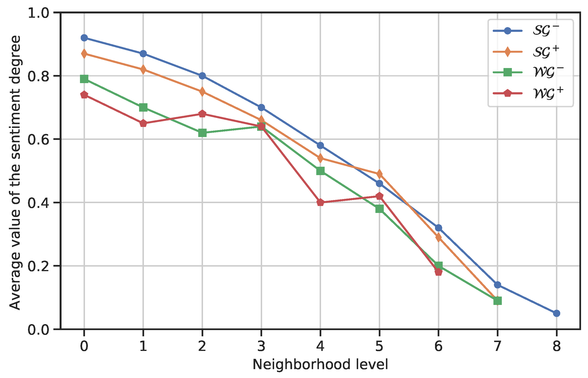
An important investigation consists in determining how the strongly positive sentiment degree varies as we move away from n i in SG + . To do this, we can consider the neighborhood of level λ , 1 λ d , d = d i a m e t e r ( SG + ) , obtained by applying the function ν on n i , λ and SG + . For each neighborhood, it is then possible to compute the average strongly positive sentiment degree of the nodes belonging to it. Generally, if there were no interference, as we move away from n i , the average strongly positive sentiment degree of a neighborhood should decrease because the influence that n i exerts on nodes tends to decrease. However, it could be the case that, once we move away from n i , there is another node different from it that exerts an influence on the nodes of the neighborhood of n i . If the new “influencer” has a discordant sentiment with n i , we might see a steep decrease in the average strongly positive sentiment degree, or even a reversal of sentiment polarity. By contrast, if the new “influencer” has a concordant sentiment with n i , we may see a slowdown in the decline of the average strongly positive sentiment degree, or even a new growth of it. The correlation that can arise between two scopes is a challenging topic that is, however, beyond the objective of this paper. Here, we simply provide a tool for computing the variation in the average strongly positive sentiment degree as we move away from n i .
Let ν ( n i , λ , SG + ) be the neighborhood of level λ , 1 λ d = d i a m e t e r ( SG + ) of n i in SG + . The average positive sentiment degree δ i j λ + ¯ of ν ( n i , λ , SG + ) is defined in Equation (12):
δ i j λ + ¯ = n h ν ( n i , λ , SG + ) δ h j + s i z e ( ν ( n i , λ , SG + ) )
In other words, it is obtained by computing the average strongly positive sentiment degree of all the nodes belonging to ν ( n i , λ , SG + ) . δ i j λ + ¯ ranges in the real interval [ 0 , 1 ] ; the higher its value, the higher the strength of the average positive sentiment.
At this point, we have at our disposal a succession of values ϱ 0 + , ϱ 1 + , , ϱ d + such that ϱ 0 + = δ i j + , ϱ h + = δ i j h + ¯ , 1 h d , d = d i a m e t e r ( SG + ) . The examination of that succession can give us some interesting insights into how the average strongly positive sentiment degree evolves as we move away from n i . It takes into account the decreasing influence of n i as we move away from it, as well as the possible presence of any interference from other “influencers”.
By plotting the values of ϱ 0 + , ϱ 1 + , , ϱ d + , we get a “spectrum” of the trend of the strongly positive sentiment degree in the spatial scope of u i . In fact, several interesting pieces of information can be derived from that spectrum. These include:
  • The variation in the average strongly positive sentiment degree in the hth section of the spectrum, defined in Equation (13):
    Δ h + = ϱ h + ϱ h 1 +
  • The relative variation in the average strongly positive sentiment degree in the hth section of the spectrum, defined in Equation (14):
    Δ h + ¯ = ϱ h + ϱ h 1 + ϱ h 1 +
  • The mean variation in the average strongly positive sentiment degree in the hth section of the spectrum, defined in Equation (15):
    Δ h + ^ = ϱ h + ϱ 0 + h
  • The maximum variation in the average strongly positive sentiment degree in the hth section of the spectrum, defined in Equation (16):
    Δ M + = max h = 1 . . v | Δ h + |
  • The minimum variation in the average strongly positive sentiment degree in the hth section of the spectrum, defined in Equation (17):
    Δ m + = min h = 1 . . v | Δ h + |
Finally, we can analyze the monotonicity of the succession ϱ 0 + , ϱ 1 + , , ϱ d + . In particular, we are interested in whether it is monotonically non-increasing. This occurs when ϱ h + ϱ h 1 + . In fact, if such a condition is not satisfied, we can say that, as we move away from n i , there is at least one further “influencer” with a sentiment concordant with the one of n i that is acting on the nodes of the neighborhoods of n i . Otherwise, it could be that there is no other “influencer” interfering with n i or that such an “influencer” is present but with a discordant sentiment with the one of n i .
What we have seen now are just some of the analyses we can perform on spatial scope. They allow us to give an idea of the potential of this concept. Many other analyses could be thought of simply by applying concepts from mathematical analysis to the succession ϱ 0 + , ϱ 1 + , , ϱ d + or concepts from graph theory to the graph SG + .
Finally, it is worth emphasizing again that all the analyses we have previously done on SG + could be straightforwardly extended to SG , WG + and WG .

4.3. Determining the Temporal Scope of the Sentiment of a User on a Topic

In this section, we illustrate our approach to determine the temporal scope of the sentiment of the user u i U on a topic t j T . In Section 3.2.1, we introduced two concepts on sentiment scope, namely sentiment type and sentiment degree of u i on t j . These two concepts play a key role in the analysis of temporal scope. Recall that the sentiment type of u i on t j can be strongly positive ( s p ), weakly positive ( w p ), weakly negative ( w n ), and strongly negative ( s n ). Instead, the sentiment degree of u i on t j is given by the value of the parameter δ i j + , in case the sentiment type is s p or w p , or the value of the parameter δ i j , in case it is w n or s n .
The temporal scope of u i on t j in the time interval T [ x . . y ] can be represented by an ordered list of pairs, as shown in Equations (18)–(20).
Θ i j [ x . . y ] = [ ( τ x , θ x ) , ( τ x + 1 , θ x + 1 ) , , ( τ y , θ y ) ]
τ b = s p i f s p s ( u i , t j ) [ b ] = true w p i f w p s ( u i , t j ) [ b ] = true w n i f w n s ( u i , t j ) [ b ] = true s n i f s n s ( u i , t j ) [ b ] = true
θ b = δ i j + [ b ] i f ( s p s ( u i , t j ) [ b ] = true ) o r ( w p s ( u i , t j ) [ b ] = true ) δ i j [ b ] i f ( w n s ( u i , t j ) [ b ] = true ) o r ( s n s ( u i , t j ) [ b ] = true )
Recall that s p s ( u i , t j ) [ b ] (resp., w p s ( u i , t j ) [ b ] , w n s ( u i , t j ) [ b ] , s n s ( u i , t j ) [ b ] ) represents the projection of s p s ( u i , t j ) (resp., w p s ( u i , t j ) , w n s ( u i , t j ) , s n s ( u i , t j ) ) in the time slice T b (see Section 3.2.1). Analogously δ i j + [ b ] (resp., δ i j [ b ] ) denotes the value returned by the function σ + ( u i , t j ) (resp., σ ( u i , t j ) ) when projected in the time slice T b (see, again, Section 3.2.1).
Clearly, by moving from a time instant T b to a time instant T b + 1 the value of τ can remain unvaried or change and the value of θ can increase, decrease, or remain constant. Each combination of the trend of these two parameters at the transition from T b to T b + 1 gives us interesting information about the time trend of the sentiment degree of u i on t j . For example:
  • If both τ b and τ b + 1 are equal to s p :
    if θ b + 1 > θ b , it means that the sentiment degree is strengthening;
    if θ b + 1 = θ b , it means that the sentiment degree is static;
    if θ b + 1 < θ b , it means that, although a strongly positive sentiment still characterizes u i , it is weakening.
  • If τ b = s p and τ b + 1 = w p , it means that the posts and comments on t j published by u i in which she shows a neutral sentiment, are increasing. This increase is such that they exceed the ones in which u i shows a positive sentiment. The number of posts/comments with a positive sentiment continues to be greater than the number of posts/comments with a negative sentiment. However, at the time slice T b + 1 we are seeing a weakening of the positivity of the sentiment of u i on t j , compared to the time slice T b .
  • If τ b = s p and τ b + 1 = w n , it means that u i is changing her sentiment on t j . This change is not yet radical, since there is a prevalence of neutral posts/comments over negative ones.
  • If τ b = s p and τ b + 1 = s n , it means that u i has completely changed her sentiment on t j . The greater the gap between θ b and θ b + 1 and the greater the change occurred.
Similarly, suitable information can be extracted in case τ b = w p , τ b = w n or, finally, τ b = s p .
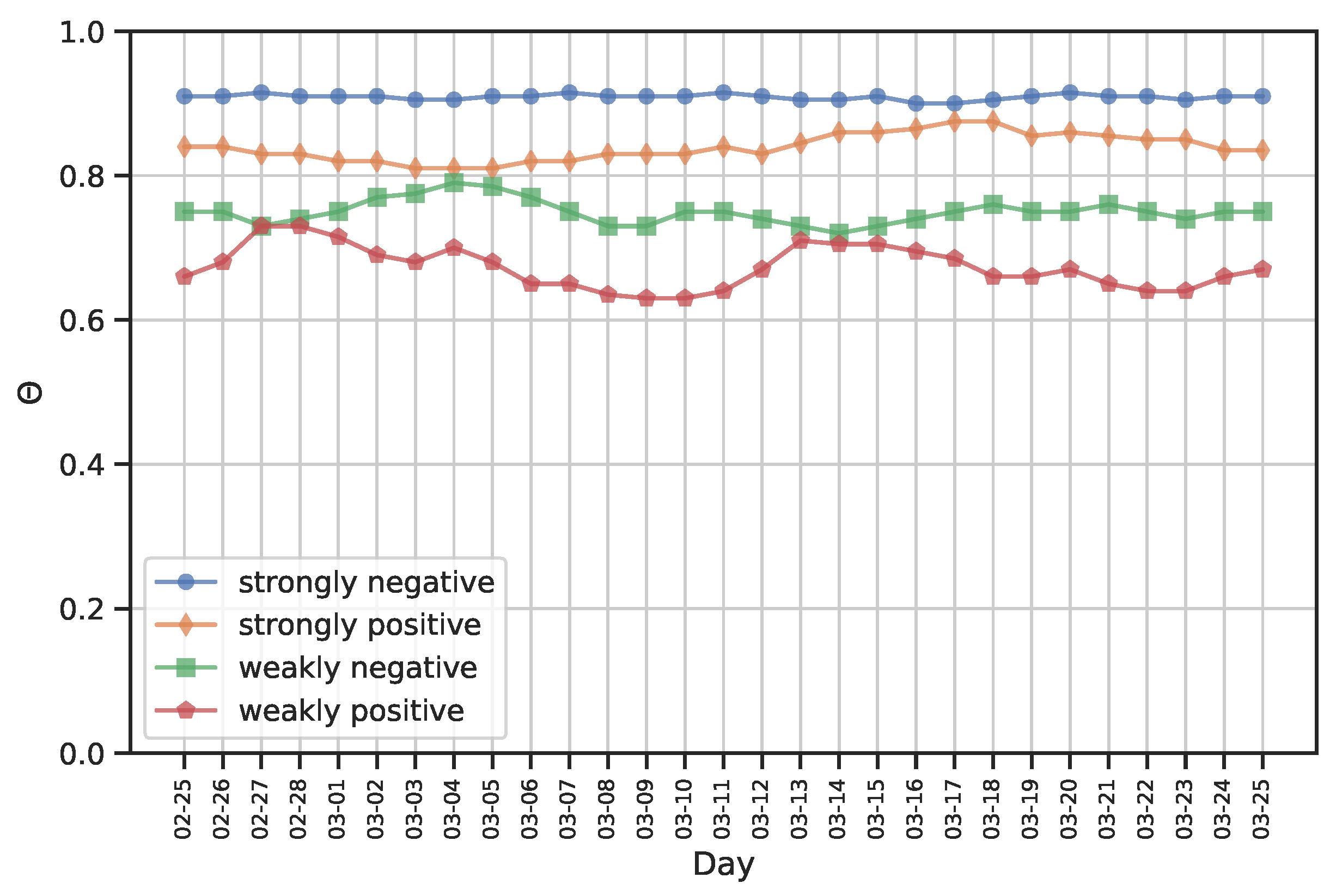
Analogously to what we have seen for spatial scope, several measures can also be defined for temporal scope. They allow us to get a quantitative view of the changes in the sentiment degree of u i on t j over a time interval. Some of these measures are the following (in defining these measures, we will refer to the time slices T b and T b 1 , instead of the time slices T b and T b + 1 , to bring their definition in line with that of the metrics for spatial scope, explained in Section 4.2.):
  • The variation in the sentiment degree between the time slices T b 1 and T b . It can be defined in Equation (21):
    Λ b = θ b θ b 1
  • The relative variation in the sentiment degree between the time slices T b 1 and T b . It can be defined in Equation (22):
    Λ b ¯ = θ b θ b 1 | θ b 1 |
  • The mean variation in the sentiment degree in the time interval T [ x . . y ] . It is defined in Equation (23):
    Λ ^ = θ y θ x y x
  • The maximum variation in the sentiment degree in the time interval T [ x . . y ] . It is defined in Equation (24):
    Λ M + = max b = x . . y | Λ b |
  • The minimum variation in the sentiment degree in the time interval T [ x . . y ] . It is defined in Equation (25):
    Λ m + = min b = x . . y | Λ b |
In addition to defining appropriate metrics to measure the change in the sentiment of u i on t j , we can check whether the succession of the values of the sentiment degree in the interval T [ x . . y ] is monotonic or not. This information must be closely coupled with that related to sentiment type. In particular, if the succession of values θ x , θ x + 1 , ⋯, θ y is monotonically non-increasing, it means that, in the time interval T [ x . . y ] , the sentiment of u i on t j is not strengthening and, rather, it is presumably decreasing. Such a decrease could cause the sentiment type to go from strongly positive to weakly positive, weakly negative, or even strongly negative. On the other hand, if the previous succession of values is monotonically non-decreasing, it means that, in the time interval T [ x . . y ] , the sentiment of u i on t j is not weakening, and, rather, it is presumably strengthening. In this case, we might see reverse transitions from the previous case, e.g., from strongly negative to weakly negative, weakly positive, and strongly positive.
The previous succession may also not be monotonic. In this case, the measures on changes in sentiment degree defined above could be extremely useful. It might also be useful to determine how often the change from one type of sentiment to another occurs, or how often the change from an increasing to a decreasing trend occurs, or vice versa.
Analogously to the spatial scope, those seen above are just some of the analyses that can be performed on the temporal scope. Many other analyses could be performed by applying the concepts of mathematical analysis or time series analysis to the succession of values θ x , θ x + 1 , ⋯, θ y .

5. Experimental Campaign

5.1. Dataset Description

To build a dataset capable of supporting our experiments, we chose Reddit as the reference social platform. We carried out such a choice because: (i) Reddit is very popular (in fact, it currently ranks 11th among the most visited sites according to Visual Capitalist (www.visualcapitalist.com (accessed on 12 September 2022))); (ii) it allows posts and comments on any topic; and (iii) its data are easily accessible through pushshift.io [59]; the latter is a data repository that allows people to download data related to Reddit comments and posts through a suitable API.
In building our dataset we focused on the posts and comments of one particular subreddit, namely /r/worldnews. The reasons for this choice lie in the fact that it has already been used as a reference subreddit in previous analyses (see Refs. [60,61,62]) and in the fact that it is one of the most complete and neutral news-related subreddits.
Specifically, through pushshift.io, we retrieved all posts and comments, along with the corresponding metadata, published in this subreddit from 25 February 2022 to 25 March 2022. The number of posts taken into account is equal to 9884 while the number of comments is equal to 633,371.
Once the data of interest were downloaded from pushshift.io, we performed ETL (Extraction, Transformation, and Loading) activities on them. Specifically: (i) we removed all posts and comments published by users who had left Reddit; (ii) we removed all posts and comments that did not have textual content or were written in a language other than English; (iii) we selected only those posts and comments related to a specific discussion theme. Regarding the latter, the choice was complex as it was important to select a specific, but sufficiently broad, theme with many facets, and thus many topics. Based on this reasoning, our choice fell on the armed conflict in Ukraine that began on 24 February 2022.
After filtering and other ETL activities, the final number of posts in the dataset is 2703, which is 27.12% of the initial ones. In contrast, the final number of comments is 82,617, which is 13.21% of the initial ones. In Table 1, we report some of the main characteristics of the final dataset. In addition to the information mentioned above, this table reports some further interesting information. In particular, we can see that the number of authors in our dataset is 4219. Among them only 119 published both posts and comments. This number is clearly very low; in particular, it is 26.50% of the authors publishing posts and 3.14% of those publishing comments.
In Figure 1, we show the distribution of comments against posts, while in Figure 2 we report the distribution of comments against score. Both figures are in log-log scale. By examining them we can observe that both distributions follow power laws. Table 2 reports the values of the corresponding coefficients α and δ .

5.2. Identification of Topics and Sentiments

In Section 3.1.1, we saw that our framework is independent of the technique used for constructing the set T of topics. In our experimental campaign, we adopted BERTopic [63] to obtain T . BERTopic is based on BERT (Bidirectional Encoder Representation from Transformers). The latter is a powerful deep learning-based framework for performing NLP tasks on texts. More specifically, it is a topic modeling technique that exploits transformers [64] and c-TF-IDF [65] to create dense clusters from which easily interpretable topics can be derived. BERTopic receives a set of documents as input and returns the list of topics covered in them. It also associates each topic thus obtained with a description and a count. The former consists of the set of words characterizing the topic. The latter indicates the number of documents mentioning it. Given a document, BERTopic is always able to determine a set of topics that characterize it.
We applied BERTopic to the 2703 posts and 82,617 comments in the dataset and obtained a set T of 101 topics. Table 3 shows some examples of the extracted topics.
After constructing the set T of topics, we turned to consider the sentiments characterizing the posts and comments published by users. In this activity, we used roBERTa-base [66]. This system was trained on approximatively 124 million tweets published from January 2018 to December 2021. Next, it was expressively fine-tuned for sentiment analysis using the TweetEval benchmark [67]. We decided to use roBERTa-base because there is a strongly similarity between the shape of texts characterizing tweets and the one of texts in posts and comments of Reddit. In fact, in both cases, we are in the presence of fast-paced messages employed to express opinions and thoughts in general.
The set of sentiments that can be derived by roBERTa-base are those typically used in sentiment analysis, namely “pos”, “neg”, and “neu”. They are also the sentiments considered in our model, as we have seen in Section 3.1. Therefore, the set S of sentiments is S = { “pos”, “neg”, “neu” }. Table 4 shows some examples of fragments, along with the corresponding sentiments, derived by roBERTa-base. Let f k be a fragment of a comment or a post (as mentioned in Section 3.1.2, f k can coincide with a whole comment or a whole post, if these are characterized by a single sentiment.) characterized by a single sentiment. Let s k be the sentiment that roBERTa-base derived for f k . Finally, let T f k be the set of topics of f k identified by BERTopic. Then, the joint use of BERTopic and roBERTa-base on f k allows us to extract a pair ( t j , s k ) for each element t j of T f k . Such a pair indicates that the sentiment s k was associated with the topic t j in f k . As previously pointed out, 101 topics were identified in our dataset. From them, 302 pairs of the type ( t j , f k ) were obtained.

5.3. Descriptive Analysis of the Graphs A , SG + , SG , WG + , and WG

In this section, we present a descriptive analysis of the graphs A , SG + , SG , WG + . and WG obtained from our dataset. This analysis allows us to identify some features of these graphs that will be useful in the next experiments. It also allows us to identify the first differences among the four graphs SG + , SG , WG + , and WG , and thus among the trends of the various sentiment types that we defined in this paper.
We begin our analysis from the graph A . Recall that this is a user-centered, single mode graph representing user interactions. Specifically, an edge in A indicates that the users associated with the corresponding nodes published at least one post or comment on the same topic and, further, that one of the two users commented on at least one post or comment of the other.
In Table 5, we report the values of some features of the graph A . In particular, we consider the number of nodes, the number of arcs, the density, and the clustering coefficient. Clearly, the number of nodes of A is equal to the number of distinct authors in the dataset, and thus to 4219. The number of arcs of A is 32,648 and, consequently, the density is 0.0018, which is a very low value. This can be explained both by taking into account the average number of comments posted by each user, which is 19.58, and by considering that the condition of existence of an arc in A is very stringent. In fact, an arc exists in A if at least one of the comments of one of its nodes refers to a post or comment of the other node. The clustering coefficient is equal to 0.0349. This value is quite high if we consider the low density of A . It implies that this graph consists of several components strongly internally connected and weakly coupled together. Some of these components may also be disconnected from all the others. This is already an interesting result found through our analysis. Indeed, it tells us that in the r/worldnews subreddit, users tend to organize themselves into high cohesive and weakly coupled communities.
Having analyzed the graph A , we now turn to the analysis of the graphs SG + , SG , WG + , and WG . As we saw in Section 4.2, each of these graphs is related to a pair ( u i , t j ) , where u i is a user and t j is a topic. The four graphs are associated with the four possible sentiment types; in particular, the  graph SG + (resp., SG , WG + and WG ) is associated with the strongly positive (resp., strongly negative, weakly positive, weakly negative) spatial scope. Essentially, these graphs represent the spatial spread of the scope related to a user u i discussing a topic t j . Recall that, given the pair ( u i , t j ) , only one of the four graphs can exist in a given time interval, depending on the sentiment type that u i had shown for t j in that time interval. Since each graph is associated with a pair ( u i , t j ) , in our analysis we considered all possible pairs of users ( u i , t j ) in the various time slices of the dataset and, for each of them, we calculated its breadth (which coincides with the number of its nodes) and its depth (which coincides with its diameter). Finally, we aggregated the results based on sentiment type, obtaining average values for each graph types. These are shown in Table 6.
The examination of this table reveals additional interesting insights. First of all, the differences among the four graphs under examination mainly concern the average breadth, while the values of the average depth are more similar. In addition, we can observe that for both the average breadth and the average depth the graphs associated with negative sentiments have higher values than the corresponding graphs associated with positive sentiments. This is in line with several researches proposed in the past literature whose authors found that negative sentiments tend to spread more easily than positive ones [68,69,70,71,72]. Finally, we can observe that, for both average breadth and average depth, the  graphs associated with weak sentiments have lower values than the corresponding graphs associated with strong ones. This is in line with other studies proposed in the past literature where it has been shown that the stronger a sentiment is, the more people resonate with it, and the likelier it is they will spread it to others [71,73,74].

5.4. Experiments on Spatial Scope

5.4.1. Variation of the Spatial Scope against the Neighborhood Level

We began our experiments on spatial scope by analyzing how it varies against the neighborhood level and whether this variation differs for the different sentiment types. To conduct this analysis we proceeded as follows.
Let us first consider the case in which the sentiment type is strongly positive. In  Section 4.2, we have seen that, in this case, the  graph representing the scope is SG + and the average positive sentiment degree of the neighbors of level λ of the user u i on the topic t j is δ i j λ + ¯ , as shown in Equation (12). We have also seen that the trend of this degree against ν is given by a succession of values ϱ 0 + , ϱ 1 + , , ϱ d + such that ϱ 0 + = δ i j + , ϱ h + = δ i j h + ¯ , 1 h d , d = d i a m e t e r ( SG + ) . In other words, this succession measures the variation of the u i ’s capability of influencing the sentiment on t j as we move away from her in the social platform, also taking into account the possible interference of other users.
In Section 5.3, we have seen that the average depth (which coincides with the average diameter) of SG + is 7.8. Therefore, in the current analysis, we consider a value of h ranging from 0 to 7.
Consider, now, all possible pairs of users ( u i , t j ) such that u i showed a strongly positive sentiment on t j . For each of these pairs, we performed all the computations specified above and constructed the succession ϱ 0 + , ϱ 1 + , , ϱ d + . The latter tells us how the average value of the sentiment degree on t j of the neighbors of level h, 0 h 7 , of the users showing a strongly positive sentiment on t j varies against the increase of h. In other words, it shows how the influence of the users having a strongly positive sentiment on t j varies as we move away from them in the social platform, also taking into account the possible interference of other users. Finally, we computed the mean of all the values of ϱ 0 + , ϱ 1 + , , ϱ d + over the possible pairs of users ( u i , t j ) . These mean values are graphically reported in Figure 3.
Similarly, we computed the succession of the mean values of the average sentiment degree on t j of the neighbors of level h of the users showing a strongly negative (resp., weakly positive, weakly negative) sentiment on t j . It indicates the variation of the influence of the users having a strongly negative (resp., weakly positive, weakly negative) sentiment on t j as we move away from them in the social platform, also taking into account the possible interference of other users. In this case, based on Table 6, h should range from 0 to 8 (resp., 6, 7). The values of this succession are graphically reported in Figure 3.
From the analysis of this figure, we can deduce several useful information about the trend of the spatial scope for the different sentiment types. As we might expect, whatever the sentiment type, as the neighborhood level increases, the average sentiment degree (and, thus, the influence of the corresponding users regarding the sentiment on a topic) decreases. As for the different types of scope, we can observe that the users with negative sentiment have a greater influence than the ones with positive sentiment, and the users with strong sentiment have a greater influence than the ones with a weak sentiment. This is in line with the results described in Section 5.3 and those found in the past literature [68,69,70,71,72,73,74].
The analysis of Figure 3 shows that the influence of users with strongly negative sentiment degree, besides being generally strong, decreases smoothly. This suggests that it is not affected by any interference from other users. When we turn to users with strongly positive sentiment degree, we can see that there is always a decrease of their influence, but this is somewhat more irregular. This indicates that the influence of this type of users may be affected, although not decisively, by the interference from other users. At some time slices, this interference can accelerate the influence decrease, while, at other time slices, it is able to slow it down. However, it is not able to reverse the trend. As for users with weak sentiment degree, we can observe that the trend is more irregular. Overall, the values are lower than the corresponding ones of the users with strongly negative sentiment degree. In addition, the interference from other users is stronger. In fact, it does not only make the decrease irregular, but is also able to reverse the trend at some points, although only for short stretches. All the peculiarities characterizing the influence of users with weakly negative sentiment degree occur even more strongly for the influence of users with weakly positive sentiment degree. In this case, the trend is even more irregular and its inversions are more frequent and pronounced.
As we have seen in Section 4.2, starting from the successions shown in Figure 3, we can derive several other interesting information. In particular, as for the succession corresponding to the average strongly positive sentiment degree, we have that:
  • Δ 1 + = 0.05 ; Δ 2 + = 0.07 ; Δ 3 + = 0.10 ; Δ 4 + = 0.12 ; Δ 5 + = 0.12 ; Δ 6 + = 0.14 ; Δ 7 + = 0.18 .
  • Δ 1 + ¯ = 0.05 0.92 = 0.05 ; Δ 2 + ¯ = 0.07 0.87 = 0.08 ; Δ 3 + ¯ = 0.13 ; Δ 4 + ¯ = 0.17 ; Δ 5 + ¯ = 0.21 ; Δ 6 + ¯ = 0.30 ; Δ 7 + ¯ = 0.56 .
  • Δ 1 + ^ = 0.87 0.92 1 = 0.05 ; Δ 2 + ^ = 0.80 0.92 2 = 0.06 ; Δ 3 + ^ = 0.07 ; Δ 4 + ^ = 0.09 ; Δ 5 + ^ = 0.09 ; Δ 6 + ^ = 0.10 ; Δ 7 + ^ = 0.11 .
  • Δ M + = m a x ( 0.05 , 0.07 , 0.10 , 0.12 , 0.12 , 0.14 , 0.18 ) = 0.18 .
  • Δ m + = m i n ( 0.05 , 0.07 , 0.10 , 0.12 , 0.12 , 0.14 , 0.18 ) = 0.05 .
Similarly, we can compute the corresponding parameter values for the other successions we examined above.
Furthermore, we can say that the successions related to SG and SG + are monotonically non-increasing. In contrast, the successions related to WG and WG + are non-monotone.
Finally, as specified in Section 4.2, many other analyses can be conducted on the successions and on the graphs SG + , SG , WG + and WG for extracting more information. For example, we can observe that the succession corresponding to WG presents only one trend reversal while the succession corresponding to WG + shows two trend reversals, which also have a larger magnitude. This also allows us to say numerically and objectively that the latter succession is more irregular than the former.

5.4.2. Relationship between Density and Clustering Coefficient and Spatial Scope

In the previous sections, we have seen some analyses allowing us to derive information on a spatial scope from its representation through a graph. In particular, we have illustrated what information on a spatial scope can be derived from the breadth and depth of the corresponding graph, as well as from the analysis of the variation of the sentiment against the neighborhood levels. In this section, we want to continue in this direction by considering some Social Network Analysis and graph theory parameters and seeing if and how they can support us in gaining a deeper understanding of scope. In particular, we will focus on density and average clustering coefficient.
In Section 5.3, we have computed the values of these two parameters for the graph A , and we have seen that they are low; then, we have provided an explanation for this behavior. In this section, we want to see what happens for the graphs SG + , SG , WG + , and WG associated with the various sentiment types.
To answer that question, we computed the density and the average clustering coefficient for all the graphs of types SG + (resp., SG , WG + , and WG ) associated with the pairs ( u i , t j ) such that u i showed a strongly positive (resp., strongly negative, weakly positive, weakly negative) sentiment on t j . Then, we averaged the values obtained for each graph type. In Table 7, we report the corresponding results.
From the analysis of this table, we can see that the values of the density and the average clustering coefficient of the graph SG + (resp., SG , WG + and WG ) are much higher than those of the graph A . This can be explained by considering how the graph SG + (resp., SG , WG + and WG ) is constructed. In fact, such a construction starts from a node serving as the root and gradually adds nodes belonging to the various neighborhoods of the root, along with the corresponding arcs, as long as the conditions expressed in the function ψ + ( ) (respectively, ψ ( ) , ξ + ( ) , ξ ( ) ) in Equation (7) (resp., (8)–(10)) are satisfied. This way of proceeding tends to favor the construction of dense and compact graphs obtained as subgraphs of the connected component of A on which their root node is located. When the boundary of the connected component is reached, the construction of SG + (resp., SG , WG + and WG ) stops. Such a construction also tends to stop when arriving at sparse areas of the graph A .
Another important information we can derive from examining Table 7 concerns the fact that the density of the graphs associated with strong sentiments is greater than that of the graphs associated with weak sentiments. This difference becomes much less marked if we consider the average clustering coefficient instead of the density. In contrast, there is no great difference between the parameters of the graphs associated with positive sentiments and those of the graphs associated with negative sentiments. This result, coupled with the ones obtained in the previous sections, suggests to us that the negativity of a sentiment is able to increase the intensity of its transmission but it is not able to increase, except marginally, the number of connections activated by users for its transmission.

5.5. Experiments on Temporal Scope

5.5.1. Variation of the Scope over Time for Each Sentiment Type

This test is dual to the one we conducted for the spatial scope in Section 5.4.1. In fact, it aims to evaluate the trend of the sentiment degree over time and how it differs for different sentiment types. The time interval we considered is the reference interval for our dataset, which is the interval from 25 February 2022 to 25 March 2022.
In Section 4.3, we have seen that, given a user u i and a topic t j , the temporal scope of u i on t j in the time interval T [ x . . y ] is represented by an ordered list of pairs (see Equation (18)), one for each time slice in the interval. The generic pair ( τ b , θ b ) denotes the sentiment type ( τ b ) and the sentiment degree ( θ b ). Recall that our model associates only one sentiment type with a user u i and a topic t j in a time slice T b . Both values can vary when passing from one time slice to another.
We carried out this experiment as follows: given a time slice T b (which coincided in practice with a day of the time interval relative to our dataset), we identified all possible pairs ( u i , t j ) such that, in the time interval T b , the user u i expressed a sentiment on the topic t j . Then, for each of these pairs, we determined the sentiment type τ i j b expressed by u i on t j in T b and the corresponding sentiment degree θ i j b .
At this point, we partitioned the pairs ( u i , t j ) based on the corresponding sentiment types in T b and, for each partition, we computed the average value of the sentiment degree. In this way, we obtained four average values of sentiment degree, i.e.,  θ b s n ¯ , θ b s p ¯ , θ b w n ¯ and θ b w p ¯ , one for each sentiment type. Finally, we repeated these tasks for each time slice of the considered interval. The results obtained are shown in Figure 4, while in Table 8 we report the values of some statistical measures computed over the whole time period of interest for the four cases under consideration.
From the analysis of Figure 4 and Table 8 we can derive some interesting knowledge patterns on temporal scope. First, we observe that the values of the average sentiment degree are generally very high, since they range from a maximum of 0.92 to a minimum of 0.63.
In addition, we can observe that the trend of the average sentiment degree for strong sentiments is generally higher than that for the corresponding weak sentiments. In fact, Table 8 shows that the average sentiment degree is equal to 0.91 and 0.84 for strong sentiments, while it is equal to 0.75 and 0.67 for weak ones. This confirms what we had already found in Section 5.4.1 for spatial scope. In addition to this, we can observe that the trend over time for strong sentiments is more constant than for weak ones. In fact, in Table 8, we can see that the standard deviation of the sentiment degree is equal to 0.003 and 0.018 for strong sentiments, while it is equal to 0.017 and 0.029 for weak ones. This is a new knowledge pattern about the trend of sentiment degree that we were able to obtain thanks to the introduction of temporal scope in this paper. It is in line with the previous results in the literature regarding strong and weak sentiments [71,73,74]. It can be explained by considering that strong sentiments correspond to very marked polarizations, and thus are unlikely to change over time, contrary to what happens for weak sentiments.
A second interesting result that can be observed from Figure 4 and Table 8 concerns the trends of negative versus positive sentiments. In fact, we can observe that the values of negative sentiment degrees are on average higher than those of positive sentiment degrees. As evidence of this, Table 8 shows that the average sentiment degree is equal to 0.91 and 0.75 for negative sentiments, while it is equal to 0.84 and 0.67 for positive ones. This represents a confirmation of the results already found for the spatial scope in Section 5.4.1. In addition to this, we can observe that the time trend for negative sentiments is more constant than that for the corresponding positive sentiments. In fact, in Table 8 the standard deviation of the sentiment degree is equal to 0.003 and 0.017 for negative sentiments, while it is equal to 0.018 and 0.029 for positive ones. The latter knowledge pattern is new to the literature and could only be extracted due to the introduction of temporal scope. It is in line with the previous results found in the literature regarding positive and negative sentiments [68,69,70,71,72].
By integrating all the derived information, it follows that the strongest and most stable sentiment is the strongly negative one; it is unlikely to be changed over time. In contrast, the ficklest sentiment is the weakly positive one. Indeed, it can be modified over time by acting appropriately on users. As for the modification possibility, the strongly positive and the weakly negative sentiments lie somewhere between the two extremes.

5.5.2. Analysis of User Stereotypes

In the previous section, we focused on the temporal variation of the average values of sentiment degree. Instead, in this section, we want to analyze the temporal variation of the sentiment degree of single users on specific topics. In particular, we want to define some user stereotypes and check whether and to what extent they are present in our dataset. More specifically, the stereotypes we define are reported in Table 9. It is worth pointing out that these are stereotypes defined by us taking into consideration the semantics of the various sentiment types and the potential usefulness of them. However, new stereotypes may be defined in the future, should the need arise.
After defining stereotypes, we computed how many users in our dataset could be associated with each of them. Recall that our dataset includes 4219 users and 101 topics. The number of potential pairs ( u i , t j ) , such that u i is a user and t j is a topic, is 426,119, while the number of actual pairs in the dataset is 130,794. The number of users associated with the various stereotypes that we defined is reported in Table 10.
From the analysis of this table, we can deduce some interesting insights. First, we observe that: (i) the number of sn-users (resp., super-sn-users) is greater than the one of sp-users (resp., super-sp-users); (ii) the number of wn-users (resp., super-wn-users) is greater than the one of wp-users (resp., super-wp-users); (iii) the number of np-users (resp., super-np-users) is greater than the one of nn-users (resp., super-nn-users). This is in line with what we have seen in the previous sections and in the literature regarding the trend of positive and negative user sentiments. Similarly, we can observe that: (i) the number of sn-users (resp., super-sn-users) is greater than the one of wn-users (resp., super-wn-users); (ii) the number of sp-users (resp., super-sp-users) is greater than the one of wp-users (resp., super-wp-users). This result is also in line with what we have seen in the previous sections and in the literature regarding strong and weak sentiments.
On the other hand, it is interesting to note that the number of w-users (resp., super-w-users) is greater than the one of s-users (resp., super-s-users). This might seem a contradiction to the previous results in this section and to the ones in the previous sections. In fact, this is not the case; this phenomenon can be explained by taking into account that the sentiments w p and w n are somewhat “contiguous”. Therefore, it is easier for a user to switch from one to the other without ever reaching strong sentiments. In contrast, the sentiments s p and s n are extreme; to be s-user or super-s-user, one could have to oscillate between these two extreme sentiments without ever going through the weak sentiments that lie in between. This is much more difficult than a context in which a user oscillates between two weak sentiments.
A further observation concerns the very low number of swinging users. This is explained by the fact that it is really difficult for a user to have four different sentiment types on the same topic. Even the number of super-s-users is so low that we can assume that their presence is more of a bias than anything else.
Finally, it is worth pointing out that more than half of the users in our dataset are p-users. In our opinion, this is an extremely positive result because it tells us that the users in our dataset were really able to express the full range of possible sentiments depending on the reference topic and time slice.

5.5.3. Discussion

In this section, we present a discussion regarding the framework proposed in this paper. In particular, we present a brief overview of its main strengths, limitations, and practical applications.
Regarding the first point, the main strengths of our framework are the following: (i) it defines a multi-dimensional view of the concept of scope; (ii) it can operate on any social platform as long as the messages exchanged in the latter are predominantly text-based; and (iii) it can assess the scope of user sentiment on any topic.
Our framework also has some limitations. Specifically: (i) it operates on only one social platform at a time, whereas the various platforms are currently interconnected because many users join simultaneously on multiple platforms, acting as bridges among them; (ii) it can currently handle only two possible dimensions, namely space and time; (iii) it is unable to evaluate and analyze the possible interference that different users may exert on a given user in defining her sentiment on a topic; (iv) it is based on text analysis and, consequently, works on social platforms where the messages exchanged are predominantly textual.
A first possible practical application of our framework involves supporting information diffusion. In fact, the knowledge of scope and its dynamics can facilitate in identifying new strategies to spread certain messages as widely as possible. A second application, dual to the previous one, consists in countering fake news. The latter, in fact, often arouse a strongly negative sentiment. Exploiting this characteristic and the concept of scope makes it possible to define an approach for identifying fake news and countering their spread. Last but not least, one could use our framework in order to identify certain user stereotypes (think, for instance, of the swinging and posed users introduced in Section 5.5.2).

6. Conclusions

In this paper, we have proposed a framework to determine the spatial and temporal scope of the sentiment of a user on a topic in a social platform. First, we have presented the concept of scope and we have seen that it summarizes several concepts, such as centrality, reputation, and diffusion, introduced in the past Social Network Analysis literature. In fact, all these concepts represent different aspects of the concept of scope. Then, we have introduced the concept of scope of the sentiment of a user on a topic and we have defined a model capable of representing and handling a multi-dimensional view of scope. Afterwards, we have proposed a set of parameters and an approach for evaluating the spatial and the temporal scope of the sentiment of a user on a topic in a social platform. Finally, we have performed a set of tests to evaluate the proposed framework on a real dataset obtained from Reddit.
The main novelties of this paper are the following: (i) it proposes a multi-dimensional view of scope, particularizing it to space and time dimensions; (ii) it introduces the concept of scope of the sentiment of a user on one or more topics; and (iii) it presents a general framework for extracting information about the scope of the sentiment of a user on topics of any subject; this framework is capable of operating on any social platform.
The main results and findings obtained by applying our framework on our Reddit dataset can be summarized as follows: (i) negative sentiments tend to spread more easily than positive ones; (ii) strong sentiments tend to spread more easily than weak ones; (iii) the influence of a user on the sentiment felt by her neighbors tends to decrease when the neighbors’ distance from her increases; (iv) users with negative sentiments influence their neighbors more than users with positive sentiments; (v) users with strong sentiments influence their neighbors more than users with weak sentiments; (vi) the influence of users with strongly negative sentiment is not affected by any interference from other users; (vii) the negativity of a sentiment can increase the intensity of its transmission but cannot increase the number of connections activated by users for its transmission; (viii) the temporal trend for strong sentiments is more constant than the one for weak sentiments; (ix) the average degree of strong sentiments over time is generally higher than the average degree of weak sentiments; (x) the average degree of negative sentiments over time is generally higher than the average degree of positive sentiments; (xi) the time trend of negative sentiments is more constant than the one of positive sentiments; (xii) the number of users with negative sentiments is greater than the number of users with positive sentiments; (xiii) the number of swinging users (i.e., users who felt all the four possible sentiment types for the same topic) is negligible; and (xiv) the number of posed users (i.e., users who were capable of feeling the full range of sentiments depending on the topic) is very high.
The ideas proposed in this paper have several possible future developments. First, we plan to extend the concepts proposed here from a single network to a Social Internetworking System, that is, a set of interrelated networks in which each user may join one or more of them. Second, we would like to study further dimensions of the scope of the sentiment of a user on a topic in a social network, in addition to the spatial and temporal ones considered in this paper. Third, we would like to further study the interference of multiple users on the sentiment of a user u i on a topic t j . In particular, we would like to analyze the case in which the interfering users are very close, as well as the case in which they have high scope and, therefore, the interference caused by each of them may be significant or, even, decisive. Last but not least, we plan to investigate the possible use of our framework to health economics applications [75] and computational linguistics [76].

Author Contributions

Conceptualization, G.B. and L.V.; methodology, F.C. and D.U.; software, L.S.; validation, E.C. and M.M.; formal analysis, G.B. and F.C.; investigation, E.C. and D.U.; resources, M.M. and L.V.; data curation, G.B. and E.C.; writing—original draft preparation, F.C. and L.V.; writing—review and editing, M.M. and D.U.; visualization, L.S.; supervision, G.B., E.C. and M.M.; project administration, F.C., D.U. and L.V. All authors have read and agreed to the published version of the manuscript.

Funding

This research received no external funding.

Institutional Review Board Statement

Not applicable.

Informed Consent Statement

Not applicable.

Data Availability Statement

We used data accessible through pushshift.io.

Conflicts of Interest

The authors declare no conflict of interest.

References

  1. Leggio, D.; Marra, G.; Ursino, D. Defining and investigating the scope of users and hashtags in Twitter. In Proceedings of the International Conference on Ontologies, DataBases, and Applications of Semantics (ODBASE 2014), Amantea, Italy, 27–31 October 2014; pp. 674–681. [Google Scholar]
  2. Cauteruccio, F.; Cinelli, L.; Fortino, G.; Savaglio, C.; Terracina, G.; Ursino, D.; Virgili, L. An Approach to Compute the Scope of a Social Object in a Multi-IoT Scenario. Pervasive Mob. Comput. 2020, 67, 101223. [Google Scholar] [CrossRef]
  3. Kempe, D.; Kleinberg, J.; Tardos, É. Maximizing the spread of influence through a social network. In Proceedings of the International ACM SIGKDD Conference on Knowledge Discovery and Data Mining (KDD 2003), Washington, DC, USA, 24–27 August 2003; pp. 137–146. [Google Scholar]
  4. Ma, Z.; Sun, A.; Cong, G. Will this #Hashtag be Popular Tomorrow? In Proceedings of the ACM SIGIR International Conference on Research and Development in Information Retrieval (SIGIR 2012), Portland, OR, USA, 12–16 August 2012; pp. 1173–1174. [Google Scholar]
  5. Ma, Z.; Sun, A.; Cong, G. On Predicting the Popularity of Newly Emerging Hashtags in Twitter. J. Am. Soc. Inf. Sci. Technol. 2013, 64, 1399–1410. [Google Scholar] [CrossRef]
  6. Miller, Z.; Dickinson, B.; Deitrick, W.; Hu, W.; Wang, A.H. Twitter Spammer Detection Using Data Stream Clustering. Inf. Sci. 2014, 260, 64–73. [Google Scholar] [CrossRef]
  7. Romero, D.; Galuba, W.; Asur, S.; Huberman, B. Influence and passivity in social media. In Proceedings of the International Conference on World Wide Web (WWW’11), Hyderabad, India, 28 March–1 April 2011; pp. 113–114. [Google Scholar]
  8. Weng, J.; Lim, E.; Jiang, J.; He, Q. TwitterRank: Finding Topic-sensitive Influential Twitterers. In Proceedings of the ACM International Conference on Web Search and Data Mining (WSDM 2010), New York, NY, USA, 3–6 February 2010; pp. 261–270. [Google Scholar]
  9. Cataldi, M.; Caro, L.D.; Schifanella, C. Emerging Topic Detection on Twitter Based on Temporal and Social Terms Evaluation. In Proceedings of the International Workshop on Multimedia Data Mining (MDMKDD 2010), Washington, DC, USA, 25 July 2010; pp. 4–13. [Google Scholar]
  10. Qasem, Z.; Jansen, M.; Hecking, T.; Hoppe, H. On the detection of influential actors in social media. In Proceedings of the International Conference on Signal-Image Technology & Internet-Based Systems (SITIS’15), Sorrento, Italy, 26–29 November 2015; pp. 421–427. [Google Scholar]
  11. Yue, L.; Chen, W.; Li, X.; Zuo, W.; Yin, M. A survey of sentiment analysis in social media. Knowl. Inf. Syst. 2019, 60, 617–663. [Google Scholar] [CrossRef]
  12. Pozzi, F.A.; Fersini, E.; Messina, E.; Liu, B. Challenges of sentiment analysis in social networks: An overview. Sentim. Anal. Soc. Netw. 2017, 1–11. [Google Scholar] [CrossRef]
  13. Yadav, A.; Vishwakarma, D. Sentiment analysis using deep learning architectures: A review. Artif. Intell. Rev. 2020, 53, 4335–4385. [Google Scholar] [CrossRef]
  14. Birjali, M.; Kasri, M.; Beni-Hssane, A. A comprehensive survey on sentiment analysis: Approaches, challenges and trends. Knowl.-Based Syst. 2021, 226, 107134. [Google Scholar] [CrossRef]
  15. Cortis, K.; Davis, B. Over a decade of social opinion mining: A systematic review. Artif. Intell. Rev. 2021, 54, 4873–4965. [Google Scholar] [CrossRef]
  16. Basile, V.; Cauteruccio, F.; Terracina, G. How dramatic events can affect emotionality in social posting: The impact of COVID-19 on reddit. Future Internet 2021, 13, 29. [Google Scholar] [CrossRef]
  17. Lai, M.; Tambuscio, M.; Patti, V.; Ruffo, G.; Rosso, P. Stance polarity in political debates: A diachronic perspective of network homophily and conversations on Twitter. Data Knowl. Eng. 2019, 124, 101738. [Google Scholar] [CrossRef]
  18. Ramachandran, D.; Parvathi, R. A novel domain and event adaptive tweet augmentation approach for enhancing the classification of crisis related tweets. Data Knowl. Eng. 2021, 135, 101913. [Google Scholar] [CrossRef]
  19. Jelodar, H.; Wang, Y.; Yuan, C.; Feng, X.; Jian, X.; Li, Y.; Zhao, L. Latent Dirichlet Allocation (LDA) and topic modeling: Models, applications, a survey. Multimed. Tools Appl. 2019, 78, 15169–15211. [Google Scholar] [CrossRef] [Green Version]
  20. Vayansky, I.; Kumar, S. A review of topic modeling methods. Inf. Syst. 2020, 94, 101582. [Google Scholar] [CrossRef]
  21. Qiang, J.; Qian, Z.; Li, Y.; Yuan, Y.; Wu, X. Short Text Topic Modeling Techniques, Applications, and Performance: A Survey. IEEE Trans. Knowl. Data Eng. 2022, 34, 1427–1445. [Google Scholar] [CrossRef]
  22. Ravi, K.; Ravi, V. A survey on opinion mining and sentiment analysis: Tasks, approaches and applications. Knowl.-Based Syst. 2015, 89, 14–46. [Google Scholar] [CrossRef]
  23. Tsvetovat, M.; Kouznetsov, A. Social Network Analysis for Startups: Finding Connections on the Social Web; O’Reilly Media, Inc.: Newton, MA, USA, 2011. [Google Scholar]
  24. Moazzami, D. Toughness of the Networks with Maximum Connectivity. J. Algorithms Comput. 2015, 46, 51–71. [Google Scholar]
  25. Khoshnood, A.; Moazzami, D. A Survey on Tenacity Parameter—Part I. J. Algorithms Comput. 2021, 53, 181–196. [Google Scholar]
  26. Moazzami, D.; Khoshnood, A. A Survey on Tenacity Parameter—Part II. J. Algorithms Comput. 2022, 54, 47–72. [Google Scholar]
  27. Bonchi, F.; Castillo, C.; Gionis, A.; Jaimes, A. Social network analysis and mining for business applications. ACM Trans. Intell. Syst. Technol. (TIST) 2011, 2, 1–37. [Google Scholar] [CrossRef] [Green Version]
  28. Scott, J. Social network analysis: Developments, advances, and prospects. Soc. Netw. Anal. Min. 2011, 1, 21–26. [Google Scholar] [CrossRef]
  29. Cantini, R.; Marozzo, F.; Talia, D.; Trunfio, P. Analyzing political polarization on social media by deleting bot spamming. Big Data Cogn. Comput. 2022, 6, 3. [Google Scholar] [CrossRef]
  30. Bayrakdar, S.; Yucedag, I.; Simsek, M.; Dogru, I.A. Semantic analysis on social networks: A survey. Int. J. Commun. Syst. 2020, 33, e4424. [Google Scholar] [CrossRef]
  31. Pankong, N.; Prakancharoen, S.; Buranarach, M. A combined semantic social network analysis framework to integrate social media data. In Proceedings of the International Conference on Knowledge and Smart Technology (KST’12), Chonburi, Thailand, 7–8 July 2012; pp. 37–42. [Google Scholar]
  32. Xia, Z.; Bu, Z. Community detection based on a semantic network. Knowl.-Based Syst. 2012, 26, 30–39. [Google Scholar] [CrossRef]
  33. Ismail, H.; Khalil, A.; Hussein, N.; Elabyad, R. Triggers and Tweets: Implicit Aspect-Based Sentiment and Emotion Analysis of Community Chatter Relevant to Education Post-COVID-19. Big Data Cogn. Comput. 2022, 6, 99. [Google Scholar] [CrossRef]
  34. Yeasmin, N.; Mahbub, N.I.; Baowaly, M.K.; Singh, B.C.; Alom, Z.; Aung, Z.; Azim, M.A. Analysis and Prediction of User Sentiment on COVID-19 Pandemic Using Tweets. Big Data Cogn. Comput. 2022, 6, 65. [Google Scholar] [CrossRef]
  35. Poulopoulos, V.; Wallace, M. Social Media Analytics as a Tool for Cultural Spaces—The Case of Twitter Trending Topics. Big Data Cogn. Comput. 2022, 6, 63. [Google Scholar] [CrossRef]
  36. Gallacher, J.; Bright, J. Hate Contagion: Measuring the spread and trajectory of hate on social media. PsyArXiv 2021. [Google Scholar] [CrossRef]
  37. Yin, F.; Xia, X.; Pan, Y.; She, Y.; Feng, X.; Wu, J. Sentiment mutation and negative emotion contagion dynamics in social media: A case study on the Chinese Sina Microblog. Inf. Sci. 2022, 594, 118–135. [Google Scholar] [CrossRef]
  38. Pröllochs, N.; Bär, D.; Feuerriegel, S. Emotions explain differences in the diffusion of true vs. false social media rumors. Sci. Rep. 2021, 11, 22721. [Google Scholar] [CrossRef]
  39. Almars, A.; Li, X.; Zhao, X. Modelling user attitudes using hierarchical sentiment-topic model. Data Knowl. Eng. 2019, 119, 139–149. [Google Scholar] [CrossRef]
  40. Yang, Z.; Kotov, A.; Mohan, A.; Lu, S. Parametric and non-parametric user-aware sentiment topic models. In Proceedings of the International ACM SIGIR Conference on Research and Development in Information Retrieval (SIGIR’15), Santiago, Chile, 9–13 August 2015; pp. 413–422. [Google Scholar]
  41. Naskar, D.; Mokaddem, S.; Rebollo, M.; Onaindia, E. Sentiment analysis in social networks through topic modeling. In Proceedings of the International Conference on Language Resources and Evaluation (LREC’16), Portorož, Slovenia, 23–28 May 2016; pp. 46–53. [Google Scholar]
  42. Liu, B.; Zhang, L. A survey of opinion mining and sentiment analysis. In Mining Text Data; Springer: Boston, MA, USA, 2012; pp. 415–463. [Google Scholar]
  43. Neves-Silva, R.; Gamito, M.; Pina, P.; Campos, A.R. Modelling influence and reach in sentiment analysis. Procedia CIRP 2016, 47, 48–53. [Google Scholar] [CrossRef] [Green Version]
  44. Carvalho, J.; Rosa, H.; Brogueira, G.; Batista, F. MISNIS: An intelligent platform for twitter topic mining. Expert Syst. Appl. 2017, 89, 374–388. [Google Scholar] [CrossRef] [Green Version]
  45. Ferrara, E.; Yang, Z. Quantifying the effect of sentiment on information diffusion in social media. PeerJ Comput. Sci. 2015, 1, e26. [Google Scholar] [CrossRef]
  46. Zhao, K.; Yen, J.; Greer, G.; Qiu, B.; Mitra, P.; Portier, K. Finding influential users of online health communities: A new metric based on sentiment influence. J. Am. Med. Inform. Assoc. 2014, 21, e212–e218. [Google Scholar] [CrossRef] [Green Version]
  47. Cao, N.; Lu, L.; Lin, Y.; Wang, F.; Wen, Z. Socialhelix: Visual analysis of sentiment divergence in social media. J. Vis. 2015, 18, 221–235. [Google Scholar] [CrossRef]
  48. Kušen, E.; Strembeck, M.; Cascavilla, G.; Conti, M. On the influence of emotional valence shifts on the spread of information in social networks. In Proceedings of the IEEE/ACM International Conference on Advances in Social Networks Analysis and Mining (ASONAM ’17), Sydney Australia, 31 July–3 August 2017; pp. 321–324. [Google Scholar]
  49. Zafarani, R.; Cole, W.D.; Liu, H. Sentiment propagation in social networks: A case study in livejournal. In Proceedings of the International Conference on Social Computing, Behavioral Modeling, and Prediction (SBP’10), Bethesda, MD, USA, 29 March–1 April 2010; pp. 413–420. [Google Scholar]
  50. Melton, C.A.; Olusanya, O.A.; Ammar, N.; Shaban-Nejad, A. Public sentiment analysis and topic modeling regarding COVID-19 vaccines on the Reddit social media platform: A call to action for strengthening vaccine confidence. J. Infect. Public Health 2021, 14, 1505–1512. [Google Scholar] [CrossRef]
  51. An, L.; Zhou, W.; Ou, M.; Li, G.; Yu, C.; Wang, X. Measuring and profiling the topical influence and sentiment contagion of public event stakeholders. Int. J. Inf. Manag. 2021, 58, 102327. [Google Scholar] [CrossRef]
  52. Cai, M.; Luo, H.; Meng, X.; Cui, Y. Topic-emotion propagation mechanism of public emergencies in social networks. Sensors 2021, 21, 4516. [Google Scholar] [CrossRef]
  53. Cai, M.; Luo, H.; Meng, X.; Cui, Y. A Study on the Topic-Sentiment Evolution and Diffusion in Time Series of Public Opinion Derived from Emergencies. Complexity 2021, 2021, 2069010. [Google Scholar] [CrossRef]
  54. Xu, Y.; Li, Y.; Liang, Y.; Cai, L. Topic-sentiment evolution over time: A manifold learning-based model for online news. J. Intell. Inf. Syst. 2020, 55, 27–49. [Google Scholar] [CrossRef]
  55. Wang, X.; Jin, D.; Musial, K.; Dang, J. Topic enhanced sentiment spreading model in social networks considering user interest. In Proceedings of the AAAI Conference on Artificial Intelligence (AAAI’20), New York, NY, USA, 7–12 February 2020; Volume 34, pp. 989–996. [Google Scholar]
  56. Tsugawa, S.; Ohsaki, H. Negative messages spread rapidly and widely on social media. In Proceedings of the International Conference on Online Social Networks (COSN’15), Palo Alto, CA, USA, 2–3 November 2015; pp. 151–160. [Google Scholar]
  57. Heimbach, I.; Hinz, O. The impact of content sentiment and emotionality on content virality. Int. J. Res. Mark. 2016, 33, 695–701. [Google Scholar] [CrossRef]
  58. Majumder, N.; Poria, S.; Peng, H.; Chhaya, N.; Cambria, E.; Gelbukh, A. Sentiment and Sarcasm Classification With Multitask Learning. IEEE Intell. Syst. 2019, 34, 38–43. [Google Scholar] [CrossRef] [Green Version]
  59. Baumgartner, J.; Zannettou, S.; Keegan, B.; Squire, M.; Blackburn, J. The pushshift Reddit dataset. In Proceedings of the International AAAI Conference on Web and Social Media (ICWSM’20), Atlanta, GA, USA, 8–11 June 2020; Volume 14, pp. 830–839. [Google Scholar]
  60. Mills, R. Reddit. In Com: A Census of Subreddits. In Proceedings of the International Web Science Conference (WebSci’15), Oxford, UK, 28 June–1 July 2015; p. 49. [Google Scholar]
  61. Guimaraes, A.; Balalau, O.; Terolli, E.; Weikum, G. Analyzing the Traits and Anomalies of Political Discussions on Reddit. In Proceedings of the International Conference on Web and Social Media (ICWSM 2019), Münich, Germany, 11–14 June 2019; pp. 205–213. [Google Scholar]
  62. Horne, B.; Adali, S. The impact of crowds on news engagement: A reddit case study. In Proceedings of the International AAAI Conference on Web and Social Media (ICWSM’17), Montreal, QC, Canada, 15–18 May 2017; p. 11. [Google Scholar]
  63. Grootendorst, M. BERTopic: Neural topic modeling with a class-based TF-IDF procedure. arXiv 2022, arXiv:2203.05794. [Google Scholar]
  64. Vaswani, A.; Shazeer, N.; Parmar, N.; Uszkoreit, J.; Jones, L.; Gomez, A.N.; Kaiser, Ł.; Polosukhin, I. Attention is All you Need. Adv. Neural Inf. Process. Syst. 2017, 30. [Google Scholar] [CrossRef]
  65. Buitinck, L.; Louppe, G.; Blondel, M.; Pedregosa, F.; Mueller, A.; Grisel, O.; Niculae, V.; Prettenhofer, P.; Gramfort, A.; Grobler, J.; et al. API design for machine learning software experiences from the scikit-learn project. In Proceedings of the European Conference on Machine Learning and Principles and Practices of Knowledge Discovery in Databases (ECMP/PKDD 2013), Prague, Czech Republic, 23–27 September 2013; pp. 108–122. [Google Scholar]
  66. Loureiro, D.; Barbieri, F.; Neves, L.; Anke, L.; Camacho-collados, J. TimeLMs: Diachronic Language Models from Twitter. In Proceedings of the Annual Meeting of the Association for Computational Linguistics: System Demonstrations (ACL’22), Dublin, Ireland, 22–27 May 2022; pp. 251–260. [Google Scholar]
  67. Barbieri, F.; Camacho-Collados, J.; Anke, L.E.; Neves, L. TweetEval: Unified Benchmark and Comparative Evaluation for Tweet Classification. In Proceedings of the Findings of the Association for Computational Linguistics (EMNLP’20), Online, 16–20 November 2020; pp. 1644–1650. [Google Scholar]
  68. Yu, H.; Yang, C.; Yu, P.; Liu, K. Emotion diffusion effect: Negative sentiment COVID-19 tweets of public organizations attract more responses from followers. PLoS ONE 2022, 17, e0264794. [Google Scholar] [CrossRef]
  69. Schöne, J.P.; Parkinson, B.; Goldenberg, A. Negativity spreads more than positivity on Twitter after both positive and negative political situations. Affect. Sci. 2021, 2, 379–390. [Google Scholar] [CrossRef]
  70. Cinelli, M.; Pelicon, A.; Mozetič, I.; Quattrociocchi, W.; Novak, P.K.; Zollo, F. Dynamics of online hate and misinformation. Sci. Rep. 2021, 11, 1–12. [Google Scholar] [CrossRef]
  71. Stieglitz, S.; Dang-Xuan, L. Emotions and information diffusion in social media—sentiment of microblogs and sharing behavior. J. Manag. Inf. Syst. 2013, 29, 217–248. [Google Scholar] [CrossRef]
  72. Suh, B.; Hong, L.; Pirolli, P.; Chi, E.H. Want to be retweeted? In large scale analytics on factors impacting retweet in twitter network. In Proceedings of the International Conference on Social Computing (SOCIALCOM ’10), Minneapolis, MN, USA, 20–22 August 2010; pp. 177–184. [Google Scholar]
  73. Rimé, B. The social sharing of emotion as an interface between individual and collective processes in the construction of emotional climates. J. Soc. Issues 2007, 63, 307–322. [Google Scholar] [CrossRef]
  74. Rimé, B.; Finkenauer, C.; Luminet, O.; Zech, E.; Philippot, P. Social sharing of emotion: New evidence and new questions. Eur. Rev. Soc. Psychol. 1998, 9, 145–189. [Google Scholar] [CrossRef]
  75. Shin, E. Physician Connectedness and Referral Choice. Oxford Bulletin of Economics and Statistics; Wiley Online Library: New York, NY, USA, 2022. [Google Scholar]
  76. Ott, M.; Choi, Y.; Cardie, C.; Hancock, J. Finding deceptive opinion spam by any stretch of the imagination. arXiv 2011, arXiv:1107.4557. [Google Scholar]
Figure 1. Distribution of comments against posts (log-log scale).
Bdcc 06 00130 g001
Figure 2. Distribution of comments against score (log-log scale).
Bdcc 06 00130 g002
Figure 3. Variation of the mean value of the sentiment degree on t j of users against the neighborhood level they belong to.
Bdcc 06 00130 g003
Figure 4. Variation over time of the average value of the sentiment degree associated with each sentiment type.
Bdcc 06 00130 g004
Table 1. Some main parameters of the dataset adopted for our experiments.
ParameterValue
No. of posts2703
No. of comments82,617
No. of (distinct) authors4219
No. of (distinct) authors publishing posts449
No. of (distinct) authors publishing comments3787
No. of (distinct) authors publishing both posts and comments119
Table 2. Values of α and δ of the power law distributions for the considered dataset— * These values were computed considering the absolute values of scores.
Distribution α δ
Figure 11.84080.0419
Figure 2 (left) * 2.92620.0418
Figure 2 (right)2.03830.0136
Table 3. Some examples of the topics and their descriptions extracted by BERTopic.
TopicDescription
t 1 { invasion , invade , mission }
t 2 { nato , defence , member , treaty }
t 3 { bunker , underground }
Table 4. Some examples of fragments and their sentiments derived by roBERTa-base (swear words are partially masked).
FragmentSentiment
“It makes me hopeful too. We need to find a way to get NATO forces engaged.”pos
“But it’s a f***ing kid that got killed by that c**t”neg
“Anyone know when this interview took place? NBC has no time stamp on the video”neu
Table 5. Some basic properties of the graph A .
PropertyValue
Number of nodes4219
Number of edges32,648
Density0.0018
Clustering coefficient0.0349
Table 6. Average values of breadth and depth for the graphs SG + , SG , WG + , and WG .
Property SG + SG WG + WG
Average breadth14318789124
Average depth7.88.46.97.3
Table 7. Average values of density and average clustering coefficient for the graphs of type SG + , SG , WG + and WG .
Property SG + SG WG + WG
Average Density0.02420.02880.1620.0184
Average Clustering Coefficient0.22150.24170.19180.2012
Table 8. Values of some statistic measures computed over the whole time period for s n , s p , w n , and w p .
Parameter sn sp wn wp
Max0.920.880.790.73
Min0.900.810.720.63
Mean0.910.840.750.67
Standard deviation0.0030.0180.0170.029
Table 9. Some possible user stereotypes.
User StereotypeDefinition
sp-user (strongly positive user) on t j This is a user who always showed a sentiment of type s p on t j when she expressed her opinions during the time interval T [ x . . y ] .
sn-user (strongly negative user) on t j Similar to the sp-user but with s n instead of s p .
wp-user (weakly positive user) on t j Similar to the sp-user but with w p instead of s p .
wn-user (weakly negative user) on t j Similar to the sp-user but with w n instead of s p .
nn-user (non-negative user) on t j Similar to the sp-user but with s p or w p instead of s p (Recall that a user can show only one sentiment type on a topic t j in a time slice; however, she can show different sentiments on t j in different time slices of T [ x . . y ] ).
np-user (non-positive user) on t j Similar to the sp-user but with s n or w n instead of s p .
w-user (weak user) on t j Similar to the sp-user but with w p or w n instead of s p .
s-user (strong user) on t j Similar to the sp-user but with s p or s n instead of s p .
super-sp-user (super strongly positive user)This is a user who always showed a sentiment of type s p on all the topics she discussed during T [ x . . y ] .
super-sn-user (super strongly negative user)Similar to the super-sp-user but with s n instead of s p .
super-wp-user (super weakly positive user)Similar to the super-sp-user but with w p instead of s p .
super-wn-user (super weakly negative user)Similar to the super-sp-user but with w n instead of s p .
super-nn-user (super non-negative user)Similar to the super-sp-user but with s p or w p instead of s p .
super-np-user (super non-positive user)Similar to the super-sp-user but with s n or w n instead of s p .
super-w-user (super weak user)Similar to the super-sp-user but with w p or w n instead of s p .
super-s-user (super strong user)Similar to the super-sp-user but with s p or s n instead of s p .
sw-user (swinging user) on t j This is a user who showed all the four sentiment types on t j during T [ x . . y ] .
ss-user (super swinging user)This is a user who behaved as a sw-user on every topic she discussed during T [ x . . y ] .
p-user (posed user)This is a user who was sp-user for at least one topic, sn-user for at least a second topic, wp-user for at least a third topic, and wn-user for at least a fourth topic. In other words, she demonstrated the ability to express the full range of sentiments depending on the topic.
Table 10. Number of users associated with each stereotype.
StereotypeNumber of Users
sp-user (strongly positive user) on t j 1211
sn-user (strongly negative user) on t j 1274
wp-user (weakly positive user) on t j 1058
wn-user (weakly negative user) on t j 1142
nn-user (non-negative user) on t j 2119
np-user (non-positive user) on t j 2497
w-user (weak user) on t j 1714
s-user (strong user) on t j 1134
super-sp-user (super strongly positive user)72
super-sn-user (super strongly negative user)88
super-wp-user (super weakly positive user)48
super-wn-user (super weakly negative user)53
super-nn-user (super non-negative user)221
super-np-user (super non-positive user)244
super-w-user (super weak user)174
super-s-user (super strong user)118
sw-user (swinging user) on t j 42
ss-user (super swinging user)2
p-user (posed user)2284
Publisher’s Note: MDPI stays neutral with regard to jurisdictional claims in published maps and institutional affiliations.

