1. Introduction
The present study applies machine learning methods in a CFD-based optimization for turbine blade aerodynamics. Literature on optimization and machine learning methods used in gas turbine studies will be reviewed, followed by a summary of the motivation of the present work.
Numerical optimization has been widely used in the design and analysis of gas turbines. In some earlier studies, specific optimization algorithms have been investigated to leverage lower fidelity models to achieve fast optimization time. One study on aerodynamic wing optimization has used an approximation and model management optimization method to incorporate low fidelity, computationally cheaper models with occasional recourse to higher fidelity, more expensive models, resulting in threefold saving in optimization time [
1]. Another study adopted a similar concept, employing a trust-region approach to interleave the exact models with cheaper surrogate models during optimization iterations [
2]. These methods demonstrate the possibility of obtaining optimized solutions on a limited computational budget by incorporating lower-fidelity surrogate models. In more recent years, an increasing number of optimization studies have relied on using parametric CFD models. In optimization of the coolant flow passage of the NASA C3X vane, different designs were evaluated repeatedly through CFD runs [
3]. In the study of a marine high-pressure turbine [
4], ten design parameters controlling multi-row film cooling designs were built into the CFD model and optimized based on a non-dominated sorting genetic algorithm. Multiple studies were also conducted on ultra-super-critical steam turbines [
5,
6], in which the blade aerodynamic efficiency was optimized using 2D and 3D CFD simulations driven by Siemens’ Simcenter HEEDS commercial Sherpa optimization algorithm. A CFD-based co-optimization strategy was presented in [
7], which demonstrates a workflow for coupling different disciplines into a nested optimization loop to conduct parallel blade aerodynamic and thermal optimizations. In addition to improving turbine blade designs, optimization has also been applied to improving the operations of gas turbine engines, for instance, to find the best valve setup parameters that reduce fuel consumption [
8].
With the advancements in computer science and data storage, an increase in interest in application of machine learning methods to gas turbine designs has been observed. One area of such applications seeing increased interest has been the prediction of key performance metrics using models trained on input data gained through past simulations or experiments. In an earlier study [
9], the outlet temperature and fuel mass flow rate at different operating conditions for a 255 MW single-shaft gas turbine were predicted by building a three-layer neural network model. Another application of the Artificial Neural Network (ANN) model has been seen in a turbine film cooling study to predict the instantaneous temperature distributions along the blade surface as well as the cooling effectiveness [
10]. In another study of a jet engine power plant [
11], a machine learning method combining physics-based and measurement-driven modeling was developed and used to conduct preventive maintenance and diagnose faults. Machine learning methods were also applied to a Viper 632-43 military turbojet engine to predict the exhaust temperature using models trained on data collected from a gas turbine simulation program [
12]. Extending from predicting individual engineering metrics, machine learning has also been used to predict field quantities representing more complicated underlying physics. A method using gradient boosted trees was used to develop models of aerodynamic loads on vibrating turbine blades and demonstrated to have good agreement with detailed CFD results [
13]. In another study, the turbine surface pressure distribution was predicted using transfer learning models, which transfer knowledge from a large-scale but low-fidelity dataset to a small-scale but high-fidelity dataset, shown to have a low prediction error with reduced cost [
14]. Machine learning has also been applied to the prediction of operating characteristics of gas turbine engines, using real-time data of power plants to develop neural networks [
15,
16]. In addition to the above applications, machine learning has also been studied to develop turbulence closure models. In one study for wake mixing, a machine learning model was demonstrated to be robust across several different operating conditions when integrated into a RANS CFD model of a low-pressure turbine [
17]. A review article on machine learning methods for science and engineering particularly highlighted the need for interpretable, generalizable, expandable, and certifiable machine learning techniques for safety-critical applications [
18].
Recent works have also focused on using machine learning embedded into design optimization procedures. In the optimization of a centrifugal compressor impeller [
19], an ANN model was first developed using CFD and FEA data from a Design of Experiment (DOE) study. Then, the ANN model was applied in an optimization procedure, which resulted in a 1% increase in isentropic efficiency and 10% reduction in the blade stress. In another study investigating a carved blade tip [
20], 55 CFD runs were conducted to generate ANN meta models, which were then used in a genetic algorithm routine to optimize the blade tip shape. In a missile control surface optimization study [
21], machine learning, reinforcement learning, and transfer learning were integrated into the optimization procedure and leveraged CFD in the evaluation iterations. In another study of 2D airfoil optimization [
22], a deep convolutional generative adversarial network was trained and embedded as a surrogate model in an optimization framework. In still another study of a compact turbine rotor [
23], machine learning models were trained and used to optimize the efficiency and torque based on a gradient-based multi-objective optimization algorithm. In addition to using machine learning models in optimization, several CFD and optimization studies have compared machine learning models with response surface models (RSM). In a study of aircyclone optimization [
24], it is concluded that ANN offers an alternative and powerful approach to response surface methods for modeling the cyclone pressure drop, benchmarked against experimental data. In another study of modeling and optimizing a perforated baffle used for turbine blade passage cooling [
25], both ANN and RSM methods were found capable of predicting friction factor and Nusselt number values, although the RSM method performed slightly better than ANN in that study. A more recent study on cyclone optimization also tested a RSM and several machine learning models. A GMDH-neural network model was found to be superior and chosen for the optimization process [
26].
As discussed in the above literature, optimization that leverages high-fidelity CFD simulations can provide accurate and realistic optimal designs in general. While leveraging a neural network as a surrogate to replace the CFD evaluations in the optimization loop can significantly improve the computational time, the fundamental challenge is that a neural network model is a lower fidelity model compared to a CFD simulation, and therefore, it may not be as accurate as CFD in predicting certain design variants required by the optimization process. Further, neural network models may also be trained based on previously available datasets that come from different studies, such as 1D and 2D simulation data, and experimental data, all of which will result in the neural network being a reduced order model compared to 3D CFD. As such, relying solely on the neural network when the predictive accuracy is necessary can lead to errant results. The present study presents a nested optimization workflow that can leverage both neural networks and high-fidelity, 3D CFD simulations at the same time to ensure every “best” design is studied in detail by the CFD tool. The introduction of a neural network into the optimization allows for over 70% reduction in the number of CFD evaluations and thus makes significant reductions in computational cost compared to a process relying exclusively on CFD simulations. The methodology is demonstrated through an aerodynamic optimization using a rebuilt model of the NASA/General Electric E3 high pressure turbine blade [
27,
28,
29].
2. Methodology
Artificial Neural Network models are used alongside 3D CFD simulations in a numerical optimization procedure to improve the aerodynamic performance of a turbine blade. ANN models are typically trained using large datasets obtained from previous experimental or numerical studies. In companies/organizations that conduct R&D on engineering designs, these datasets are usually available from previous studies. The present study proposes a methodology of using such existing knowledge from previous studies to train ANN models and then use the ANN models in an CFD-based design optimization process. A dataset from a previously published work is obtained to conduct the ANN modeling training in the present study. The overall framework of the research methodology is shown in
Figure 1, which illustrates how different analysis models/tools required by the optimization process are created. First, data were obtained from a previous study [
7] containing 3204 CFD design evaluations of different 2D turbine blade profiles. Performance metrics including efficiency and power were extracted as targets, with the blade geometric parameters serving as input features, to train ANN models. The ANN hyperparameters were subsequently optimized. The blade cross-sectional profiles were parameterized using a Class-Shape Transformation (CST) method [
30]. Using the 2D blade cross-sectional profile, the 3D blade CAD geometry was created with additional parameterization allowing for the variation of further design transformation, such as the thickness, twist, and lean. The blade CAD geometry was then used to build a 3D Reynolds Averaging Navier–Stokes (RANS) CFD model, which solves for the flow field in a single blade passage. Once the ANN models and the 3D CFD simulation are independently developed, they are integrated into a nested optimization procedure for repeated evaluations of different blade design variants to optimize the design parameters. In the nested optimization process, an inner optimization loop is executed using the ANN models to improve the blade cross-sectional profile. In each iteration of the global optimization, the best blade profile is selected from the inner optimization step to create a 3D CFD blade model with additional parameters such as the scaling factors, twist, and lean angles. The optimization targets improving the efficiency and power of the blade. Details of the optimization process will be discussed in a later session in this chapter.
2.1. Artificial Neural Network
A dataset representing different design variants of 2D aerodynamic CFD results was obtained from a previous study [
7] and used to train ANN models. The dataset features blade design and performance parameters for 3204 designs. The input parameters for the ANN models include 20 blade design parameters. These parameters are the weighting factors used by the CST method [
30] to control variations in the blade profile. Under the CST method, these weighting factors are multiplied by Bernstein polynomials to define a shape function, and then subsequently multiplied by a class function to define the aerodynamic blade profile. An order-9 Bernstein polynomial was deemed sufficiently flexible for the purposes of the study [
7] and that choice is repeated here, resulting in 10 design parameters for each of the suction and pressure sides of the blade:
and
. These 20 parameters are used as input features in the ANN models and optimization parameters in the subsequent blade optimization process. Two performance metrics in the dataset were used as output parameters, isentropic efficiency, and power output, for which two ANN models were developed, respectively. The efficiency and power are defined based on enthalpy quantities of the flow, as follows:
The Keras API for TensorFlow [
31] was used to construct the ANN models. In consideration of the different distributions of the efficiency and power data and the robustness of the model, a separate ANN model was constructed for each of these two quantities. After some preliminary tests on ANN models of 5, 6, and 7 layers, 7 and 6 layers were constructed, respectively, into the ANN models representing efficiency and power. The choice of the number of layers in ANN usually varies in different problems. It will be shown that the prediction errors are within acceptable range for the chosen number of layers, and that the errors will be further reduced by optimizing the hyperparameters of the models. The first layer of each ANN model has 20 inputs representing the blade input features (CST weights) and the last layer has one output, which is either efficiency or power. The number of neurons in the hidden layers of each ANN, along with other topological and training parameters, were optimized in a separate hyperparameter optimization process. As a starting point for that process, the hyperparameters for each ANN model were set using the values provided in the first two columns of
Table 1.
To improve the predictive performance of the ANN, the hyperparameters were optimized using Siemens commercial optimization tool HEEDS and its Sherpa algorithm [
32]. A diagram of the optimization process is provided in
Figure 2. The optimizer repeatedly tunes all the hyperparameters for the ANN models listed in the index column of
Table 1 with an objective to minimize the model test error on a held-out testing dataset. In each optimization cycle, the dataset is randomly split into a training and testing set with a ratio of 95/5. The training set is used the train the ANN model. The training process involves a typical backpropagation procedure with an 80/20 split of the training set, over multiple epochs with TensorFlow’s ADAM optimizer. After the training step is completed, the model’s performance is then evaluated against the held-out test set. The evaluation error is passed back to the optimization solver to tune the hyperparameters for the next cycle. A total number of 240 iterations were executed during the optimization of each of the two ANNs. The evaluation number, 240, was based on the Sherpa algorithm best practice [
32], which recommends the number of evaluations being about 10 times the number of input variables for single objective optimization problems, due to the hybrid and adaptive methods employed by the algorithm. In the ANN optimization, 12 hyperparameters must be optimized, and thus it requires at least 120 evaluations according to the best practice. In consideration of the relatively fast run time for the ANN training process in comparison to the 3D CFD run time, that evaluation number is further doubled to 240 to provide better accuracy.
The optimized hyperparameters are obtained and provided in the last two columns of
Table 1. After optimization, the evaluation errors for efficiency and power were reduced, respectively, from 0.33% to 0.10%, and from 0.43% to 0.10%. The performance of the initial and optimized ANN models are also examined by comparing the predicted values vs. true values from the test set, shown in
Figure 3. It is observed that the optimized ANN models result in better alignment between the predicted values and the true values, as well as narrower bandwidths of the prediction errors on the histogram plots. From
Figure 3, it is also observed that the bias of the optimized ANN for efficiency was greatly reduced, as the data points are evenly distributed on both sides of the line of unity slope, shown in the second subplot. This is consistent with the histograms of the prediction errors in
Figure 4, which shows that both the bias and bandwidth of the errors were improved in the optimized ANN models. The optimized ANN models are used in the subsequent blade optimization process in this study. The Python scripts for training the ANN models with the optimized hyperparameters are provided in [
33]. The CPU time for training an individual ANN largely depends on the number of Epochs. In the present study, the CPU times for training the ANN models representing efficiency and power with their respective optimized hyperparameters were 14.3 min and 8.5 min, respectively. The total compute times for optimizing the hyperparameters of these ANN models were, respectively, 13.07 h and 11.65 h. This optimization was carried out based on parallel execution of 10 training models at the same time using a 6-core CPU.
2.2. Parametric Blade CAD and CFD Model
An initial turbine blade CAD model was built by adapting the E3 high pressure turbine blade profiles. Using the first stage rotor blade coordinates provided at three spanwise locations [
27]—hub (12.693in), pitch (13.571in), and tip (14.41in)—and accounting for the incoming flow angle [
28,
29], a 3D CAD model was constructed by lofting these cross-sectional profiles, as shown in
Figure 5a, to provide a baseline case. Applying the same philosophy of lofting cross sections and at the same time utilizing the CST method for the cross-sectional profile definition [
27], a parameterized blade CAD model was created for the design optimization study. First, the CST method creates a base cross-sectional profile, which is used as the pitch profile. The CST method allows varying the base profile in design optimization through manipulating the 20 weighting parameters,
and
. Then, the base profile is scaled to create the hub and tip profiles. In the scaling process, the twist angles and chord lengths of the hub and tip profiles are matched to their counterparts of the original E3 blade; 4 additional scaling factors,
, were applied to the lower and upper profiles of the hub and tip sections, respectively, to allow for small variations of the thicknesses of the hub and tip sections so that they can be optimized. The ranges of these variations are defined conservatively out of practical considerations of the original E3 engine blade shape. In general, the scaling allows the hub profile to be thicker and the tip profile to be thinner. Finally, a tilt angle,
, and a lean angle,
, were also built into the CAD model to be optimized later. Based on a reverse engineering study analyzing different engine blade geometries [
34], the tilt angle can vary from 0 to 0.164°, and the lean angle can vary from −0.086° to 0.086° in the optimization study. A schematic plot of these angles is shown in
Figure 5b.
Using the 3D blade, a single-blade passage CFD model was developed using Siemens multi-physics package Simcenter STAR-CCM+. The continuity, momentum, and fluid energy transport equations are solved using a coupled solver (density-based) following a finite volume approach with a 2nd order upwind discretization scheme on a polyhedral grid. Menter’s SST K-Omega model [
35] with all y+ treatment is used as a closure to the turbulence model. The all
y+ wall treatment adjusts the application of a turbulence wall function based on the local
y+ value of the near wall mesh cell. The CFD simulations were performed using the test conditions. Following E3 engine rotor testing conditions and 2D CFD practices from NASA studies [
28,
29], a total pressure of 344,777 Pa and a total temperature of 709 K were used for the inlet boundary condition, while an atmospheric pressure of 101,325 Pa was defined at the outlet. The same boundary conditions representing the engine testing conditions were also applied in the previous 2D CFD simulations in [
7]. (These 2D CFD datasets were used to develop ANN models in the present work.) A grid sequencing method was used to provide initial conditions, by solving inviscid flow equations repeatedly on a set of gradually refined mesh grids. Automatic CFL number control was also applied to adjust the CFL number in response to linear solver convergence behavior during the algebraic multigrid procedure. To ensure overall solution convergence is reached, in addition to monitoring the residuals of the governing fluid equations, stopping criteria were also set based on the asymptotic values of engineering quantities, such as isentropic efficiency, power output, maximum surface temperature, and total pressure difference.
The CFD methodology has been applied in a previous study based on a 2D version of the E3 blade and validated against other experimental and numerical results of the E3 blade [
7]. In the present study, a grid independence investigation has also been performed for the 3D CFD. Three sets of CFD grids with different resolutions were tested. The chosen grid features 12 million polyhedral cells with near-wall y+ values all below 1.4, based on which the solution calculates a baseline efficiency of 96.0% and a power of 5.638 × 10
4 W. (Note power is calculated based on the single blade CFD model in the current study, which has a pie sector angle of 4.737°). The relative difference between the chosen grid and its next-level refined grid is 0.1% for efficiency and 0.02% for power.
2.3. Optimization Strategy
The present study adopts a nested optimization process. The nested optimization is a slight variation of a previous co-optimization strategy introduced in [
7]. The nested optimization accomplishes two essential tasks. First, because an ANN model calculation consumes significantly less computing resources and time than a 3D CFD run, nesting an inner optimization based on the ANN model can effectively utilize the time while waiting for a 3D CFD run to complete. For each 3D CFD simulation run, 250 evaluations of different blade cross-sectional profiles were completed in the inner optimization loop using the ANN model. Second, the inner, ANN-driven optimization passes the best blade profile of the present optimization cycle to the 3D CFD run. This architecture effectively allows using the ANN-driven optimization to guide the 3D CFD search, and thus reduces the number of 3D CFD runs compared to an optimization process that is solely based on evaluating 3D CFD models.
The goal of the optimization is to maximize blade efficiency,
η, and power output, Pow. The design variables that are being explored in optimization are the ones discussed in the previous session,
,
,
,
and
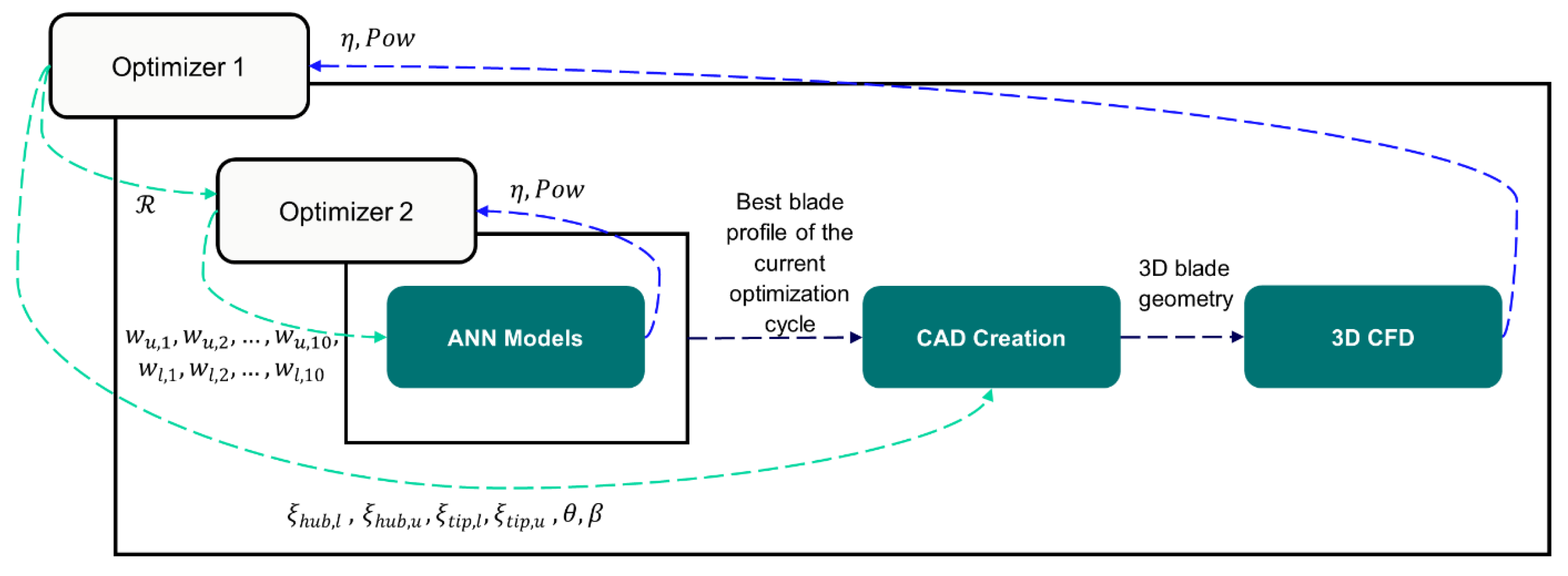
. The optimization procedure repeatedly executes the ANN and CFD models to evaluate different blade design variants, while extracting performance metrics to search for better designs. As the ANN model is much less computationally expensive compared to CFD, it is leveraged in an optimization loop by itself to yield optimized cross-sectional blade profiles, which are subsequently used to construct 3D shapes for CFD simulations. Using the ANN embedded optimization to guide the search for the best blade profiles allows for reducing the number of expensive CFD evaluations. As such, a nested optimization workflow is constructed, as illustrated in
Figure 6. The workflow is realized using commercial optimization software Simcenter HEEDS and its Sherpa optimization algorithm [
30] is used in both Optimizer 1 and Optimizer 2. The Sherpa algorithm constantly evaluates the characteristics of the problem by using a hybrid combination of search strategies at each stage of the optimization process to best traverse the design landscape. In addition, it also adapts the tuning parameters of the search strategies to the specific region of the search. The HEEDS’ Sherpa algorithm has been effectively applied to optimize gas turbine applications, as shown in studies [
5,
6,
7].
In the global optimization loop (Optimizer 1 as shown in
Figure 6), a multi-objective trade-off problem is solved targeting maximizing both efficiency and power. Two constraints are set: efficiency must be greater than 95% and power must also be greater than a baseline power value. These constraints are included in the optimization performance function, based on considerations of practical gas turbine design metrics and general performance characters of the E
3 engine. The global optimization solver, Optimizer 1, affects the blade shape change by directly optimizing the section scaling factors and blade angles in the CAD. In addition, Optimizer 1 also affects an inner optimization process, which is represented by Optimizer 2. Optimization 1 controls the selection of the CST weights used as input parameters for Optimizer 2, through manipulating a random seed,
, which sets the initial state for the global search strategies employed by the Sherpa algorithm. Although Optimizer 1 does not directly manipulate the CST weights, because
controls their selection, it acts as a 1D encoding of the entire 20-dimensional design space for Optimizer 1 to explore. Optimizer 1 repeatedly evaluates and optimizes different design variables during the global optimization cycles; in each evaluation cycle, Optimizer 2 optimizes the CST weights using the ANN models, with an objective to maximize the efficiency and a constraint on minimum power value. Overall, 250 blade cross-sectional profiles were evaluated in each execution of Optimizer 2. It directly explores the shape profiles through manipulating the weighting parameters used in the CST method. In each evaluation cycle of Optimizer 1, the best blade profile found by Optimizer 2 is applied in the more expensive and high-fidelity CFD simulation. The performance function in each optimization is defined as the sum of normalized objectives minus the sum of normalized constraints. In a generic form, the performance function is formulated as follows:
In the above formula, represents the objective quantity, such as and ; represents the amount of violation resulted from each constraint definition (); the normalization factors Norm are selected using the respective and values of the baseline design.
4. Conclusions
The present study has demonstrated an optimization workflow combining the use of neural networks and high-fidelity CFD. The neural network models were trained on over three-thousand design data points from a previous publication. The practical implication of the overall strategy is that in engineering design analysis, existing data sets, which are generally available from the previous simulation, experimental, or reduced-order studies, can be leveraged to build neural network models, which can then be used in combination with high-fidelity CFD simulations to guide optimization processes. This approach achieves a reduction in the required number of high-fidelity CFD runs, and hence reduces the computational cost while maintaining accuracy. The integration of computationally inexpensive ANN models, which were evaluated 40,750 times, allows for a relatively small number (163) of CFD evaluations in the present optimization process, resulting in a total run time of about 30 h (with 6 CFD evaluations running in parallel, each consuming 160 compute cores). It is estimated that if the nested optimization strategy based on ANN was not used, a total number of 733 CFD evaluations will be required due to the large number of design variables exposed in 3D CFD evaluations, resulting in roughly 135 h of the optimization run time if the same compute resource settings were used.
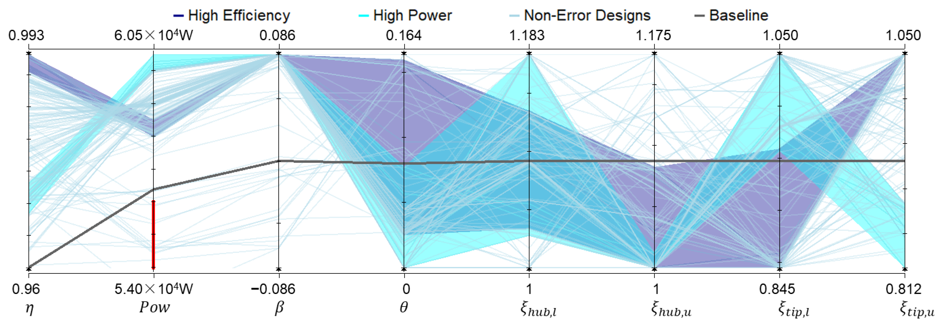
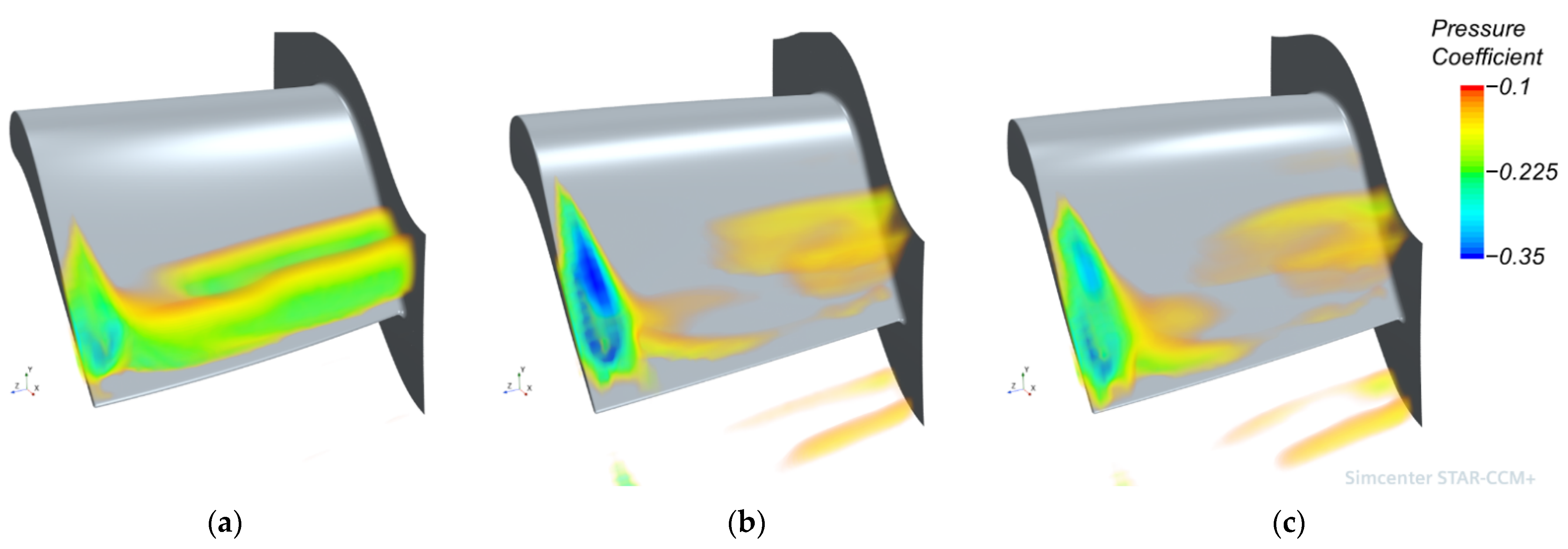
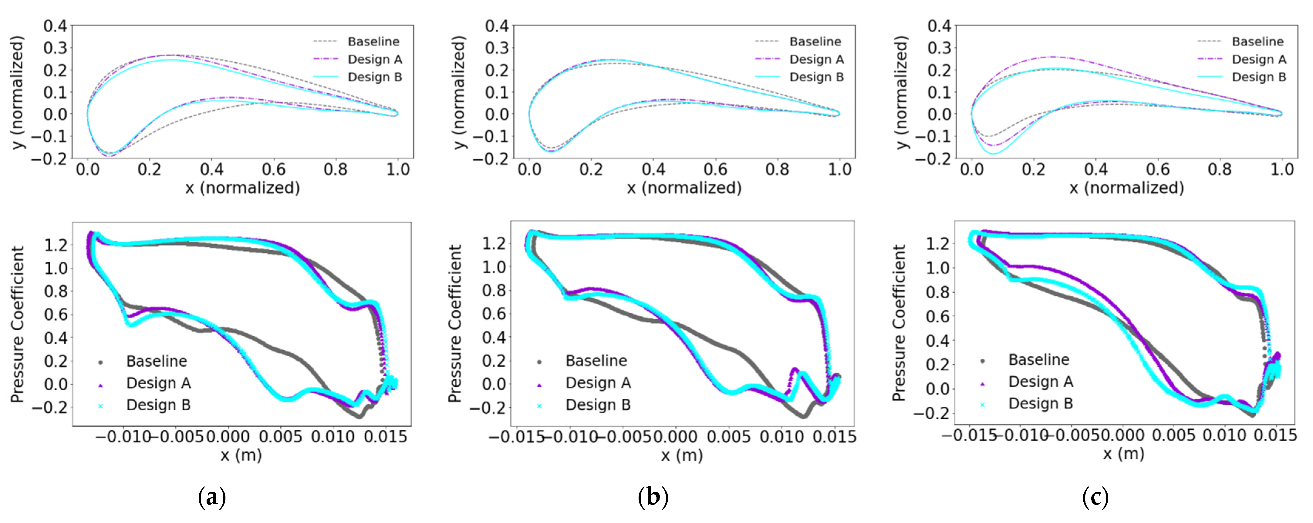
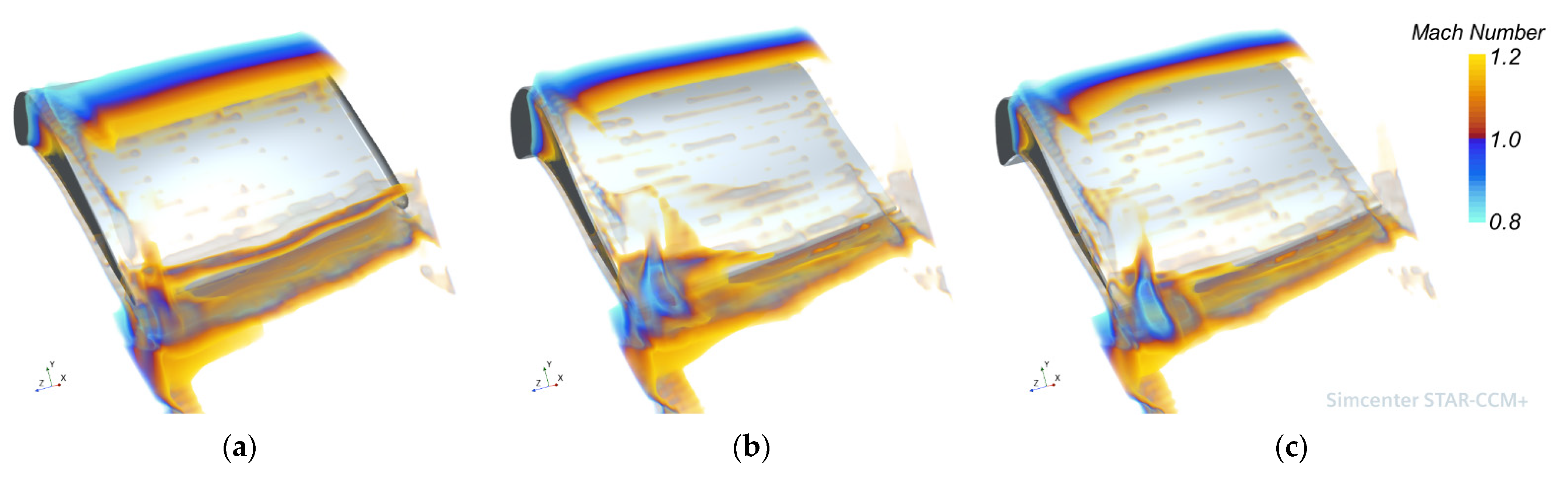
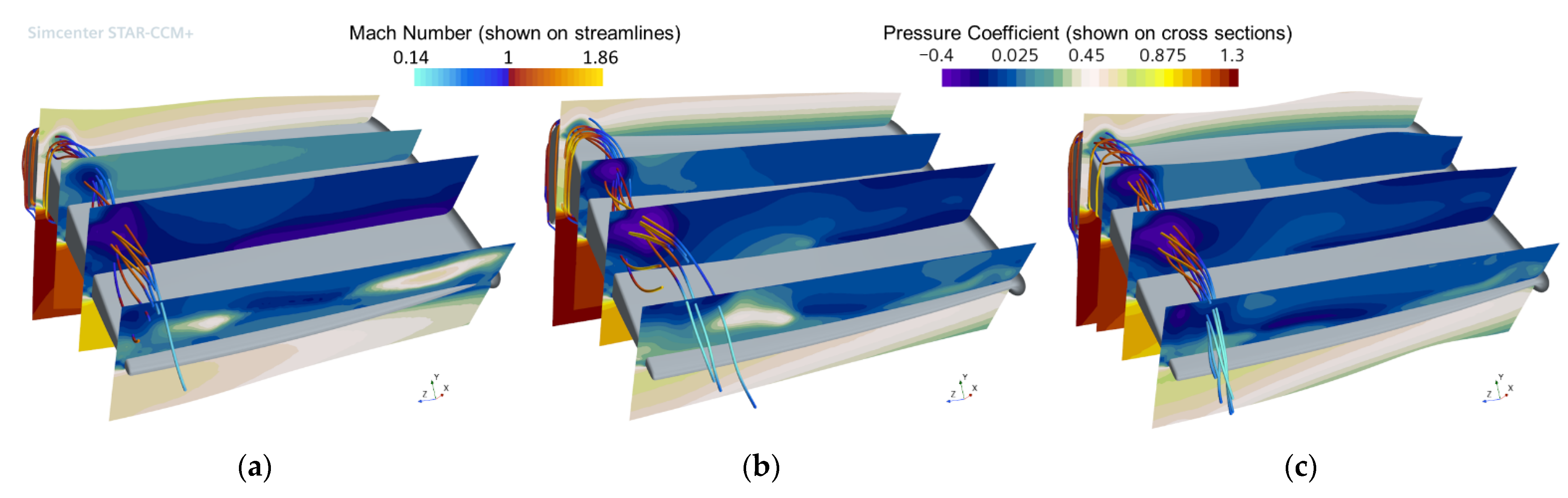
The efficacy of the methodology is demonstrated on a turbine blade aerodynamic problem. ANN models with 7 layers and 6 layers were built to represent two blade performance metrics, efficiency, and power, respectively. The hyperparameters of the ANN models were optimized, and the models were used as surrogate models along with high-fidelity CFD simulations in a nested optimization procedure to obtain optimized blade designs. Pareto front designs representing improved efficiency and power were found by the optimization procedure. A lean angle and a tip scaling factor were shown to be more favored by the optimization procedure than other parameters in the context of the chosen blade and analysis methodology used in the current study. Examining the fluid dynamics of the optimized designs vs. the baseline design reveals that the optimization (1) reduced the magnitude of the most negative pressure coefficients in the flow on the suction side near the trailing edge, and (2) altered the blade geometry that reduced the shock near the trailing edge. Both of these aspects have effects on improved efficiency and power in the optimized designs.
As a future extension of this study, the following may be considered. (1) Test the performance of other response surface methods and meta models against ANN and apply them in the nested optimization workflow. (2) The present study demonstrates a nested ANN-CFD optimization methodology, applied to an idealized turbine CFD problem as a proof-of-concept. In production-level gas turbine designs, more detailed constraints on the geometry or loading curve must be incorporated to ensure more realistic optimization outcomes. Different power output conditions of the engine may also be explored in optimization.


