Article

Calibration of Micromechanical Parameters for the Discrete Element Simulation of a Masonry Arch using Artificial Intelligence

1
Department of Structural Mechanics, Faculty of Civil Engineering, Budapest University of Technology and Economics, Műegyetem rakpart 3., H-1111 Budapest, Hungary
2
Department of Machine and Product Design, Faculty of Mechanical Engineering, Budapest University of Technology and Economics, Műegyetem rakpart 3., H-1111 Budapest, Hungary
3
Department of Artificial Intelligence, Faculty of Informatics, Eötvös Loránd University, Pázmány Péter Sétány 1/A, H-1117 Budapest, Hungary
*
Author to whom correspondence should be addressed.
Infrastructures 2023, 8(4), 64; https://doi.org/10.3390/infrastructures8040064
Submission received: 10 February 2023 / Revised: 11 March 2023 / Accepted: 20 March 2023 / Published: 24 March 2023

Abstract

:
This study focuses on an old but still unresolved problem of automatically calibrating the constitutive parameters of discrete element models. Instead of the troublesome and time-consuming manual trial-and-error method, which is typical today, the authors suggest using artificial intelligence techniques. A masonry arch is analysed, whose experimental static load–displacement behaviour is known from the literature. An attempt is made to match this behaviour with discrete element models, through finding appropriate quantitative values for the parameters. Two methods (Genetic Algorithm (GA) and Particle Swarm Optimisation (PSO)) are tested and, since PSO turns out to be more reliable, a further improved version, ‘Trust-Based Particle Swarm Optimisation’ (TBPSO), is proposed. The results show that (1) TBPSO quickly leads to suitable alternative parameter sets that make the discrete element model match the behaviour of the real experiments and (2) the optimal values of the parameters strongly depend on the loading velocity and the discretisation method used.

1. Introduction

1.1. DEM and Its Applications

The Discrete Element Method (DEM) was introduced by Cundall in 1971 [1] as an alternative to the Finite Element Method (FEM) for the mechanical analysis of systems consisting of separate solid bodies. The Discrete Element Method has been used for a wide variety of applications, including rock mechanics, granular assemblies, powder technology, industrial packaging, pharmaceuticals, mining, agriculture and Computational Fluid Dynamics (CFD) problems.
The Discrete Element Method considers the structure as a collection of separate blocks. Each block is able to move (and, in many codes, deform) independently of the others, so that large displacements of the elements follow, and the elements can make new contacts with each other while existing contacts can open up, fully or partially. Sliding can also occur between blocks. Contact forces are transmitted through contacts between neighbouring blocks, according to a wide variety of existing constitutive models. The contact creation, sliding and separation are automatically followed in DEM, which makes DEM particularly advantageous for modelling masonry structures. There are many different commercial and open-source DEM software packages; in the context of masonry mechanics, the interested reader is advised to consult the book by Sarhosis et al. [2] and Chapter 13 in Sarhosis et al. [3]. The Combined Finite Discrete Element Method by Munjiza can be considered as a combination of the FEM and DEM, see [4,5] and the references therein.

1.2. Material Parameters

The main difficulty with DEM simulations is that only very carefully selected input micromechanical material parameters result in reliable results that reflect reality. The material parameters have to be chosen in such a way that the simulation of real physical behaviour matches the measured results. To calibrate material parameters, researchers have employed different methods, largely based on manual tuning using trial and error. There is no standard way to calibrate these material parameters and very little research has been carried out on the standardisation of the methods used.
One way of choosing the correct material parameters is to directly measure them [6] at the particle level forming the analysed system (and their contacts). Some of these parameters may be easy to measure while others may be very complex. Even if all the parameters can be measured, the complexity of the measurement and the scatter of the results may be an obstacle in practice.
The other method is to perform an experiment, or a set of experiments, to determine the bulk parameters [6] of the material or structure. Numerical simulations are then performed with the same conditions as in the laboratory. The material parameters for numerical simulation are repeatedly modified and adjusted until the bulk behaviour obtained from the simulations matches that of the actual experiments.
The simplest method is to use trial and error to calibrate the parameters. This method can be efficient when a single parameter has to be calibrated but when the number of parameters increases the calibration process becomes complicated. The solution to such problems may not be unique and this may result in two or more different sets of parameters yielding the same bulk behaviour.
While matching the bulk behaviour of the real experiments with numerical simulations, it should be noted that the available open-source and commercial DEM codes differ in their contact treatment, element constitutive behaviour and time integration technique, etc. Therefore, the material parameters calibrated for one DEM code might not necessarily work for another.

1.3. Previous Works on Algorithmised Calibration

The majority of the work on the calibration of parameters has been carried out for granular assemblies, due to the use of these materials in pharmaceutical industries and in soil mechanics. Hardly any work has been carried out on the calibration of DEM models for masonry structures. There are empirical formulas for some parameters, but these have been developed over time for specific purposes and cannot be generalised.
The research carried out by Yoon [7], Rackl and Hanley [8], Turkia et al. [9], Zeng et al. [10], Bhalode and Ierapetritou [11] and Mohajeri et al. [12] used Design of Experiments (DoE) for the calibration of material parameters for granular materials. These are systematic methods that establish a relation between input factors (material parameters of DEM simulations) and responses (bulk behaviour or bulk material properties) using statistical techniques. The methods described by these authors used different DoE methods for the procedure. Mohajeri et al. [12] proposed a sensitivity analysis by using “one variable at a time” to find the sensitivity of the parameters to the bulk parameters. In this way, the number of variables to calibrate can be reduced. Rackl and Hanley [8] used Latin hypercube sampling, which is an even yet random distribution, to generate a set of parameters. Discrete Element Method simulation was then used to identify the bulk parameters. A statistical regression method, known as kriging [13], was used to predict the bulk parameters and the unknown set of parameters after obtaining the required data.
Benvenuti et al. [14] used the multiple layer perceptron neural network for the prediction of the angle of repose of a granular material based on DEM simulations. An initial set of parameters was used to train the neural network, with 85% training data and 15% validation data. Mean squared error was used as a loss metric for the training process.
Wesbrink et al. [15] used reinforcement learning (RL) to calibrate the parameters of granular materials. The method works on the principle of maximising reward by changing the state. The proposed method results in a faster convergence, depending on the learning factor, but since the method uses a gradient descent policy the solution obtained could be a local optimum instead of a global optimum.
Do et al. [16] and Mohajeri et al. [17] used different genetic algorithms [18] to calibrate the parameters of granular materials. Since genetic algorithms are stochastic and approximate, the accuracy of the solution cannot be quantified.
Sarhosis et al. [19] used two different methods to calibrate the parameters of the non-linear continuum–mechanical constitutive models of masonry. One of them is the iterative procedure known as Sequential Quadratic Programming, which is similar to the Newton–Raphson method. The convergence rate of such algorithms is faster but can be problematic in the case of local optimums. The other method used was a genetic algorithm, which has been discussed above.
As mentioned five graphs before, DoE methods can be used to calibrate the parameters. However, with an increasing number of variables to calibrate, the number of simulations to find the optimum set of parameters can become extensively large. In [12], a preparatory method used one variable at a time for DoE to rule out certain variables and improve the speed but the process of ruling out had to be performed manually. Deep learning methods [20] and applications have been studied more recently, but there is the problem of getting stuck in local optima and vanishing gradients. Therefore, we chose to use metaheuristic algorithms for calibration processes, as the application of these algorithms in real-life optimisation problems is very significant and well established. Another important advantage is that these methods are totally independent of the gradients of objective functions.

1.4. Modelling of Masonry Structures

The mechanical analysis of masonry structures is one of the most important fields of application of DEM. Masonry structures form a significant portion of our architectural heritage as well as of contemporary buildings and other engineering structures. In particular, masonry arches, domes and vaults are those structures where failure and damage are mainly due to the loss of stability caused by phenomena strongly related to the discrete internal composition of the structure. Due to their specific discontinuous, nonlinear nature, several alternative methods are applied in the engineering practice for their analysis, instead of or in addition to the usual (continuum-based) FEM. A thorough overview of these methods is given in D’Altri et al. [21]. Among these, Limit State Analysis (LSA) and the Discrete Element Method (DEM) are mostly used today in the literature.
The theoretical background of LSA for masonry structures was formalized by Heyman [22] assuming that masonry blocks are perfectly rigid, their contacts have no resistance to tension and there is no frictional sliding between them (more accurately, any forms of tangential relative translations have to be excluded [23]). Within LSA, basically two approaches (and their combination) can be used: lower-bound approaches, based on the “Safe Theorem” or “Static Theorem” [24], and upper-bound approaches, based on the “Unsafe Theorem” or “Kinematic Theorem” [25]. Innumerous numerical techniques can be found in the literature that use LSA, and the most sophisticated versions take into consideration cohesion and limited frictional resistance as well [26] or reinforcements [27], but there are situations when the application of LSA needs special care. The most important such issue is the “duality gap”, a phenomenon well known in plastic limit state analysis, which occurs in the case of non-associated flow rules, i.e., when the normality condition fails. In this instance, the static and kinematic theorems may lead to contradicting results. The structural behaviour becomes history-dependent, and without a history analysis the behaviour cannot reliably be assessed. The problem of the duality gap does not occur if the tangential relative translations between the blocks are completely excluded from the analysis, or if the friction angle and the dilation angle between the blocks are equal. In masonry structures, however, relative tangential translations are usually not a priori excluded by the construction method, and on the other hand the joints approximately obey the Coulomb friction law: their frictional sliding angle is usually around 35–50 degrees, while the dilation angle in the joints is only a few degrees or practically zero. Hence, a realistic contact failure law is non-associated and the phenomenon of duality gap has to be faced. Repeated attempts occur in the literature to overcome the problem of the duality gap [28,29,30]. To summarize, LSA is problematic for use in situations where the behaviour is non-associated because of the blocks being not perfectly fixed against tangential relative translations. Other problematic issues, such as partially opened joints, crosswise tension resistance depending on the magnitude of compression, etc., should also be mentioned. In these situations, DEM can be an advantageous alternative. A comparison of a FEM/DEM procedure, a nonlinear heterogeneous FEM technique and an LSA including friction is provided in [31].
The Discrete Element Method is usually applied for one of two purposes. The first of them is to simulate the behaviour of an existing structure. In this case, a DEM model is constructed using the geometrical data of the real structure, it is attempted to assign realistic material parameters and then the engineer is able to test the structural response to different mechanical effects and interventions. While the geometry of an existing structure can be fairly accurately determined (though there may be hidden parts of the structure where only approximations can be used), the material characteristics are very difficult to estimate reliably. In particular, those characteristics related to failure are the most problematic to determine. One solution is to calibrate a DEM model to another artificially created or less valuable structure on which loading procedures can be performed, including failure, and then the material parameters of the well-calibrated DEM model are modified with the help of engineering intuition according to the differences between the tested structure and the existing valuable one.
The second typical purpose for applying DEM is to support theoretical conclusions with virtual experimenting. The literature is rich in theoretical predictions such as the minimally necessary thickness for arches or vaults, the collapse modes of arches, the optimal shapes of domes, the necessary level of upfills on vaults, etc. These theoretical predictions are often supported by DEM-simulated virtual experiments. The basis of the simulations should be a reliable model of realistic structures: the material parameters in the models should be chosen in such a way that the behaviour of the models is validated on real experiments. Then, if the theoretical conclusions are confirmed by the virtual experiments, a careful sensitivity analysis can explore the range of their validity for other cases when the micromechanical material parameters are different from the calibrated ones.
In both cases, the basis of the analysis must be a DEM model whose material parameters are calibrated according to a real experiment. This calibration is, however, very time consuming if performed manually, according to the intuitive guesses of the modeller.

1.5. Aim of Study

The aim of this study is to present a calibration method that can be applied to DEM problems. This study applies the calibration process to a masonry arch. Circular masonry arches are the simplest structures that exhibit many of those stability issues and failure phenomena so characteristic to general single- and multi-span arches, domes and vaults. That is why the loading procedure of a circular masonry arch is chosen as a benchmark problem to test different calibration algorithms. Future applications of the calibration process to other masonry structures and granular assemblies are also possible. A distinct feature of DEM simulations is that they are computationally extremely expensive. Therefore, a calibration method has to be found that results in a usable outcome (i.e., a good set of material parameters) in the smallest possible number of runs of DEM simulations.
Section 2 of the present paper first introduces a laboratory experiment whose outcomes are applied as the reality to be matched with the well-calibrated DEM model. Then, the discrete element analysis by Pulatsu et al. [32] is presented, in which the parameters for their model were manually chosen. Some important remarks are made regarding the sensitivity of the behaviour of the loading velocity and the surface mesh density. These experiences are then relied on in the investigations in the later sections.
Section 3 focuses on those optimisation methods that are promising candidates for application to the calibration. Particle Swarm Optimisation (PSO) [33,34] and Genetic Algorithm (GA) [18] are the most widely used metaheuristic algorithms; hence, they are tested in their basic original form. Based on the results, a modified version of PSO (named Trust-Based Particle Swarm Optimisation (TBPSO)) is introduced. The objective function calculates the deviation between the load–displacement curves of the real experiments and their simulations. Its value is called ‘fitness’. Two versions are used for the objective function. The first one is based on the raw experimental data containing noise, i.e., the oscillations originating from the non-zero velocity and drops in force due to the stick-slip phenomenon. This version is simpler, but not advantageous to use because it often becomes stuck in local optima. The second one is based on processed experimental and simulation data that are smoothed using a neural network. This neural network is also introduced.
Section 4 compares the three calibration methods for both objective functions (using the original geometry of Pulatsu et al. [32] as well as other geometry). Our main finding is that TBPSO performs better for the current problem with the weight parameters used in the study; less iteration is needed to reach equally good solutions in both PSO and GA with a higher number of iterations. However, both TBPSO and the original PSO can be used for the purpose of the calibration of further DEM simulations. The use of GA is not recommended in its applied version; however, further studies can be undertaken to find an improved version of GA or to find the sets of numerical control parameters that work well with the calibration problems, leading to a faster convergence rate (less time to reach an optimum solution).
Finally, Section 5 summarises the most important conclusions.

2. Prototype Masonry Arch Quasi-Static Experiment and Analysis

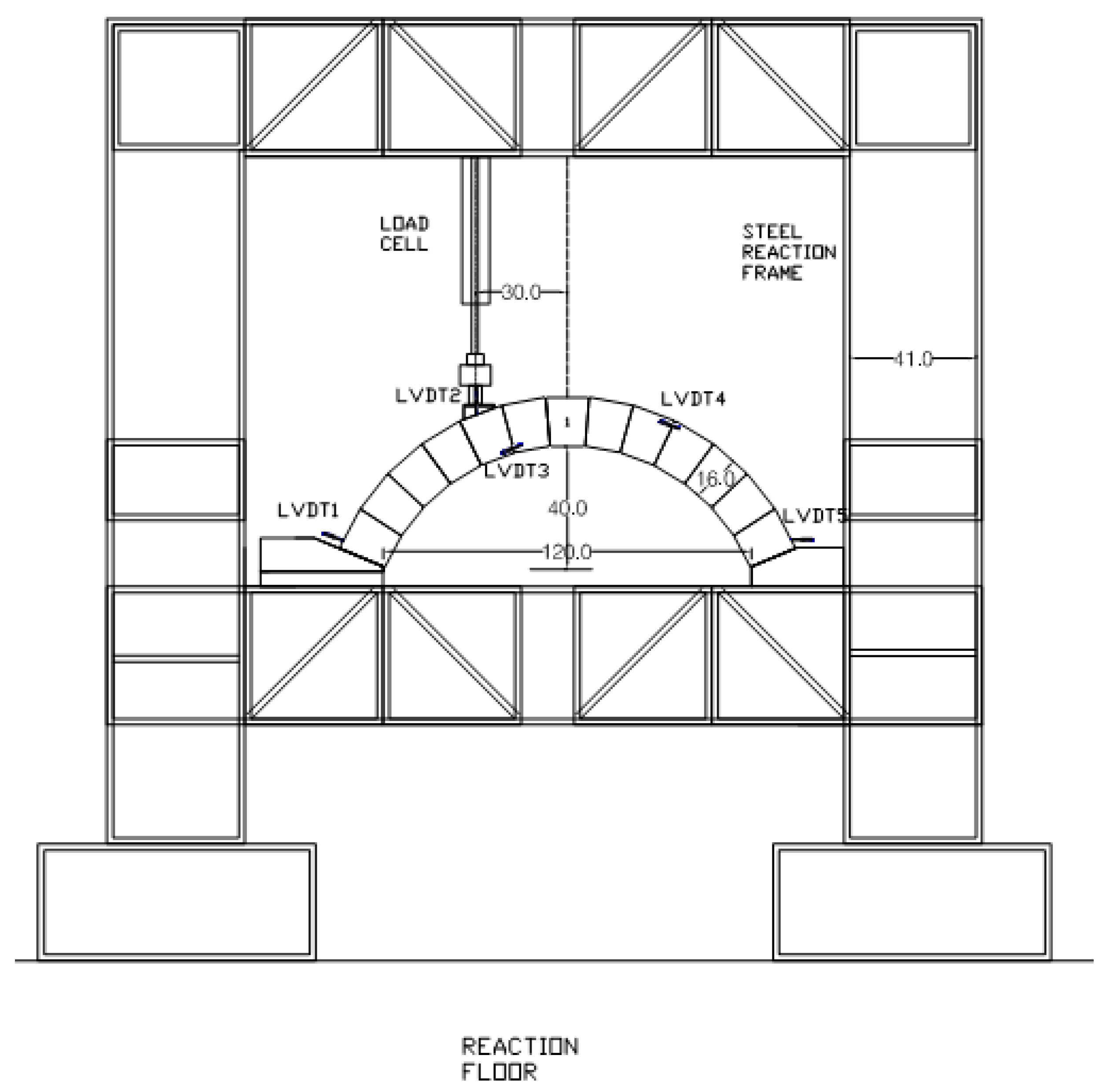
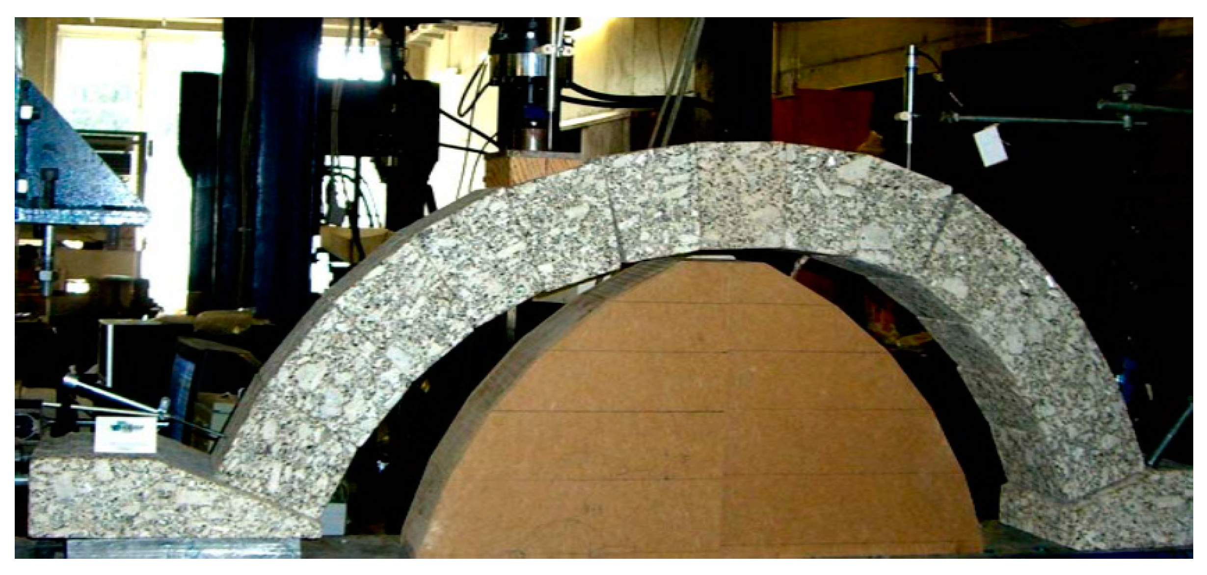
2.1. Experimental Setup of Masonry Arch

In this study, discrete element models were calibrated to match the experiment by Birhane [35], which was set up at the University of Minho, Portugal. Our analysis focused on the quasi-static range of behaviour, with the future aim of extending the calibrations to dynamic phenomena as well. The prototype stone masonry arch was originally designed to be used in impact response studies. However, the same arch geometry was also used in quasi-static experiments. The dimensions of the stone masonry arch were determined by the geometry of the drop-weight apparatus. The out-of-plane thickness of the stone masonry was WA = 200 mm. The clear span was LA = 1200 mm, and the clear height was HA = 400 mm. The arch comprised 12 voussoirs, one keystone and two abutments. The radial thickness of the arch was tA = 160 mm. The radial thickness of the arch ring and the number of stone masonry units were determined by an iterative limit analysis using RING software.
To reuse the same units for different experimental setups, the blocks were made of sound granite rock. The stones were prefabricated by the Artecanter-Indústria Criativa, Lda. stone working company. A rotary sawing machine was used to cut the units to the prescribed dimensions; therefore, the stone surfaces were jagged. The physical and material properties of the stones were given by Vasconcelos [36].
The arch was assembled on a reaction steel frame made of I-section steel beams. The height of the beams was 45 cm, and they were braced sufficiently. The strength and stiffness of the steel girders were greater than that of the masonry arch. Therefore, it was assumed that the frame would be able to provide sufficient lateral and vertical constraints to the arch.
The arch was constructed using formwork, which fitted the intrados of the arch, since it was a dry joint masonry arch. Assembly started from the left and right abutments, stacking up the units towards the keystone. The keystone was pressed in between the left and right rings using a hammer.
A wooden interface was glued to the fifth voussoir using an adhesive with a horizontal width of 110 mm, an out of plane thickness of 200 mm and a height of 50 mm on the left side. A steel bearing with a roller at the top was placed over the wooden interface to ensure that there was no rotational restraint between the arch and the actuator.
The actuator was placed at the quarter span of the arch. Five linear variable displacement transducers (LVDT) were fixed on the arch to measure displacement, as shown in Figure 1. Linear variable displacement transducers 1 and 5 were placed to measure the sliding at the abutment–arch interfaces. Linear variable displacement transducer 2 was used to measure the displacement at the loading point. Linear variable displacement transducers 3 and 4 were placed to measure the opening at rotational hinges on both quarter spans.

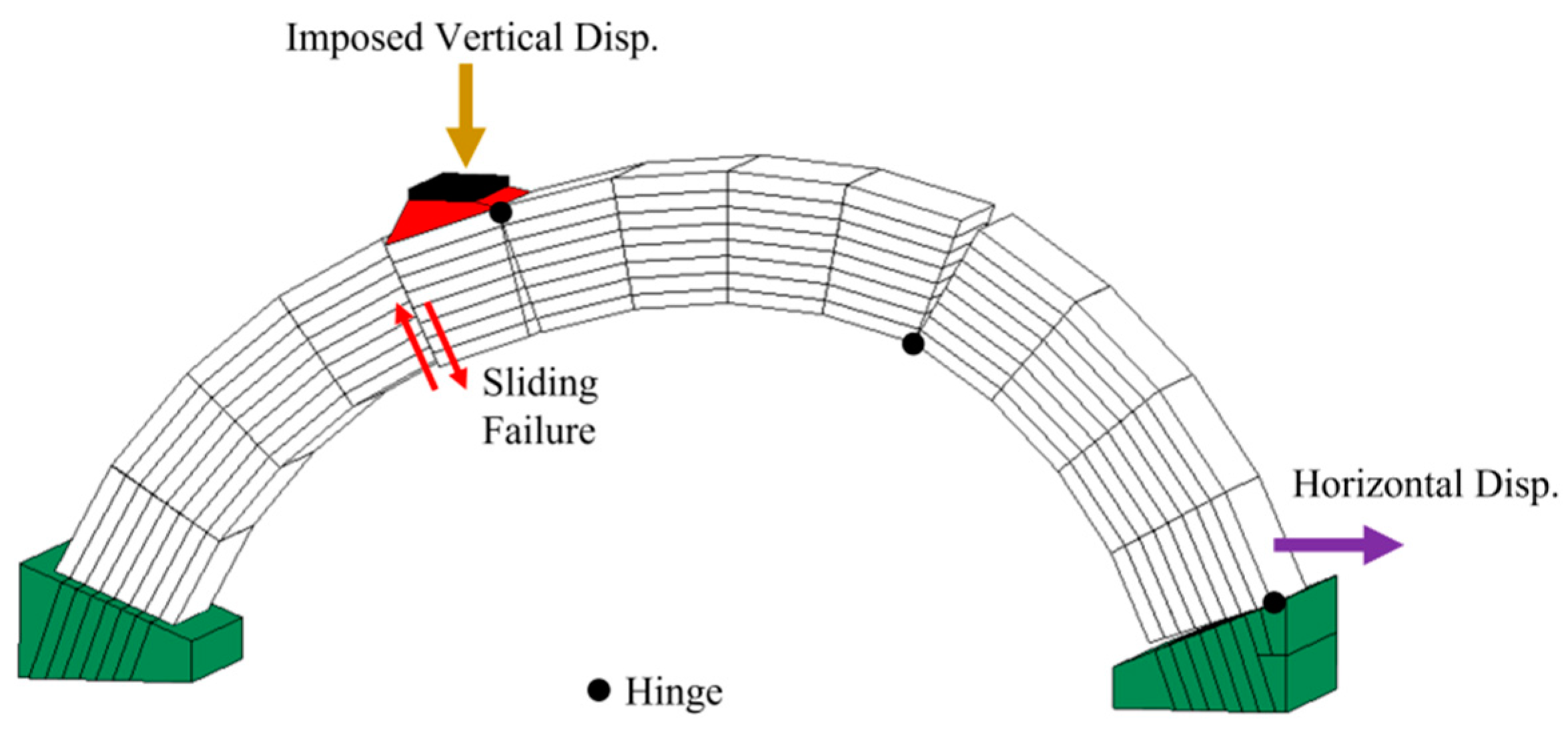
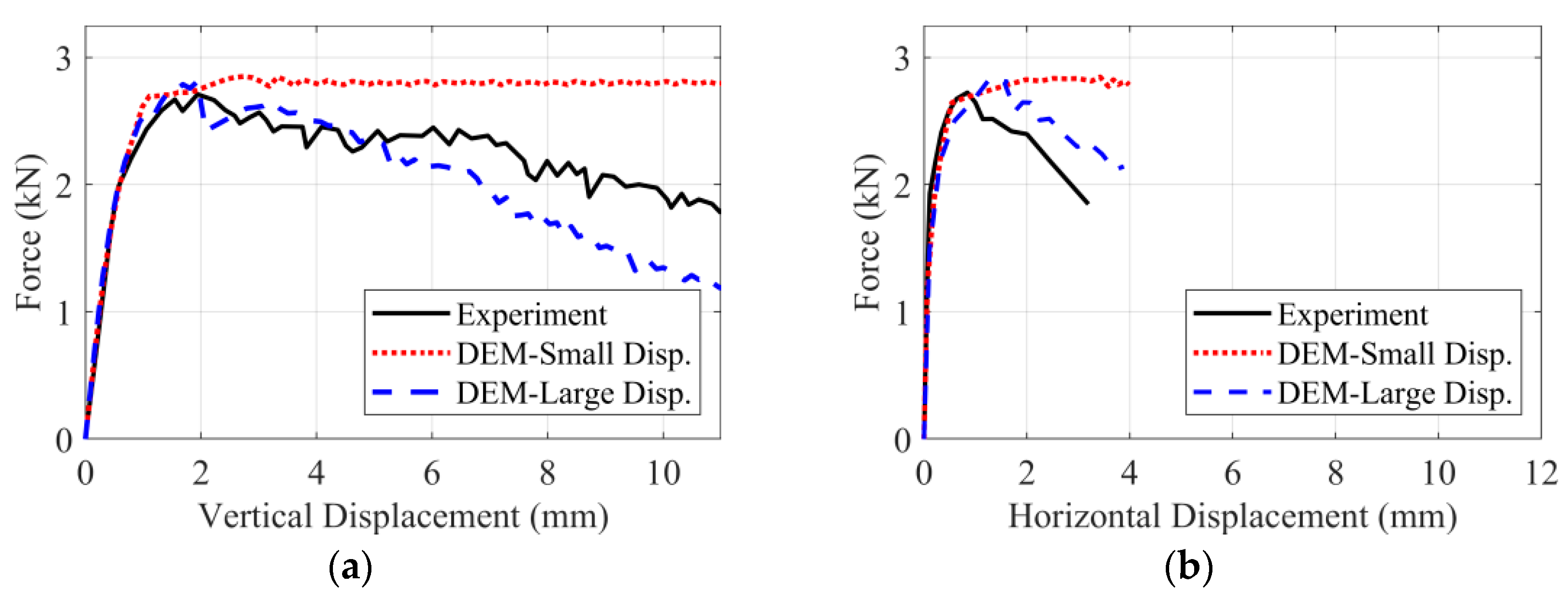
2.2. Quasi-Static Experiment and Results

In the quasi-static experiment, a displacement-controlled load was applied in the loading cell at a constant loading rate of 0.005 mm/s. The loading rate was determined to achieve stable progressive damage to the arch. The test was stopped after 2361 s, at the maximum vertical displacement of 12 mm, and the arch did not collapse. The peak load was measured as 2.71 kN. The peak strength of the arch was decreased by 35%. Three rotational hinges and one sliding hinge were observed, as shown in Figure 2: two rotational hinges at the left and right quarter span, one rotational hinge at the right abutment–arch interface and one sliding hinge at the left quarter span.

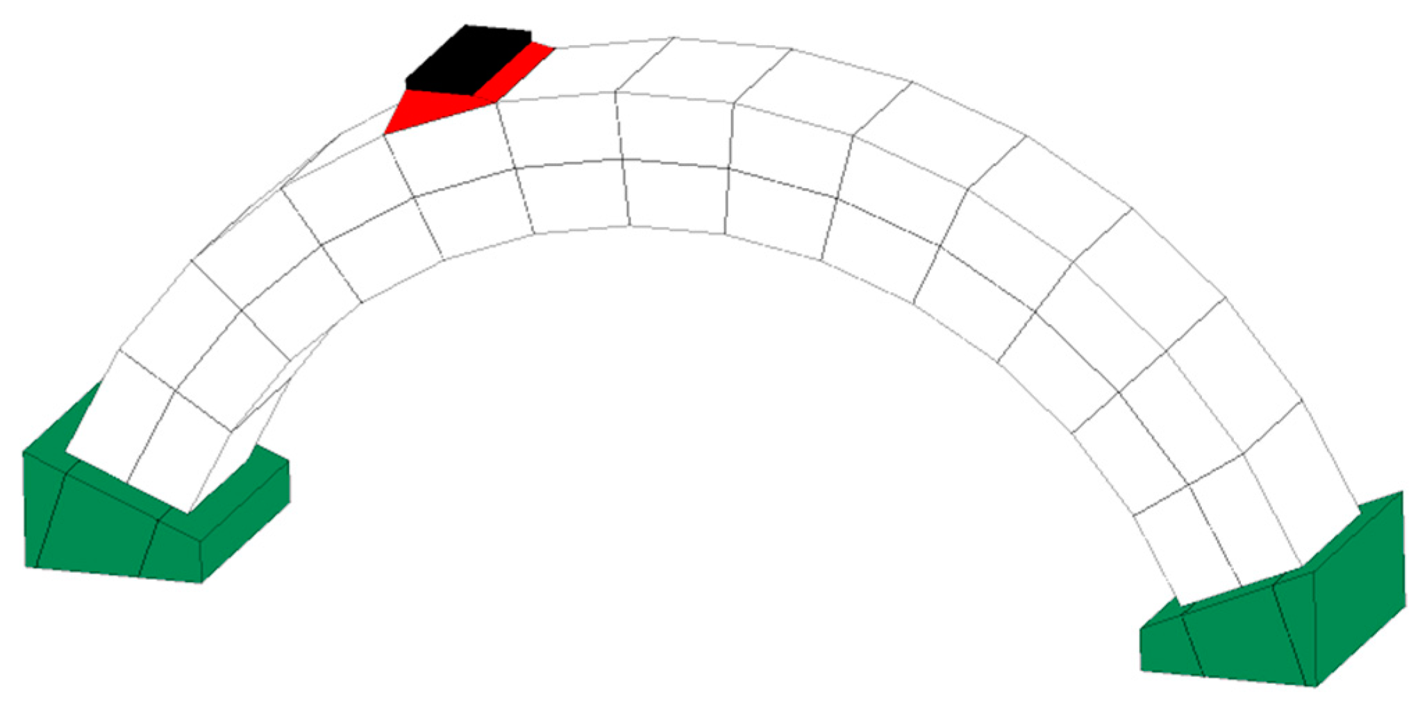
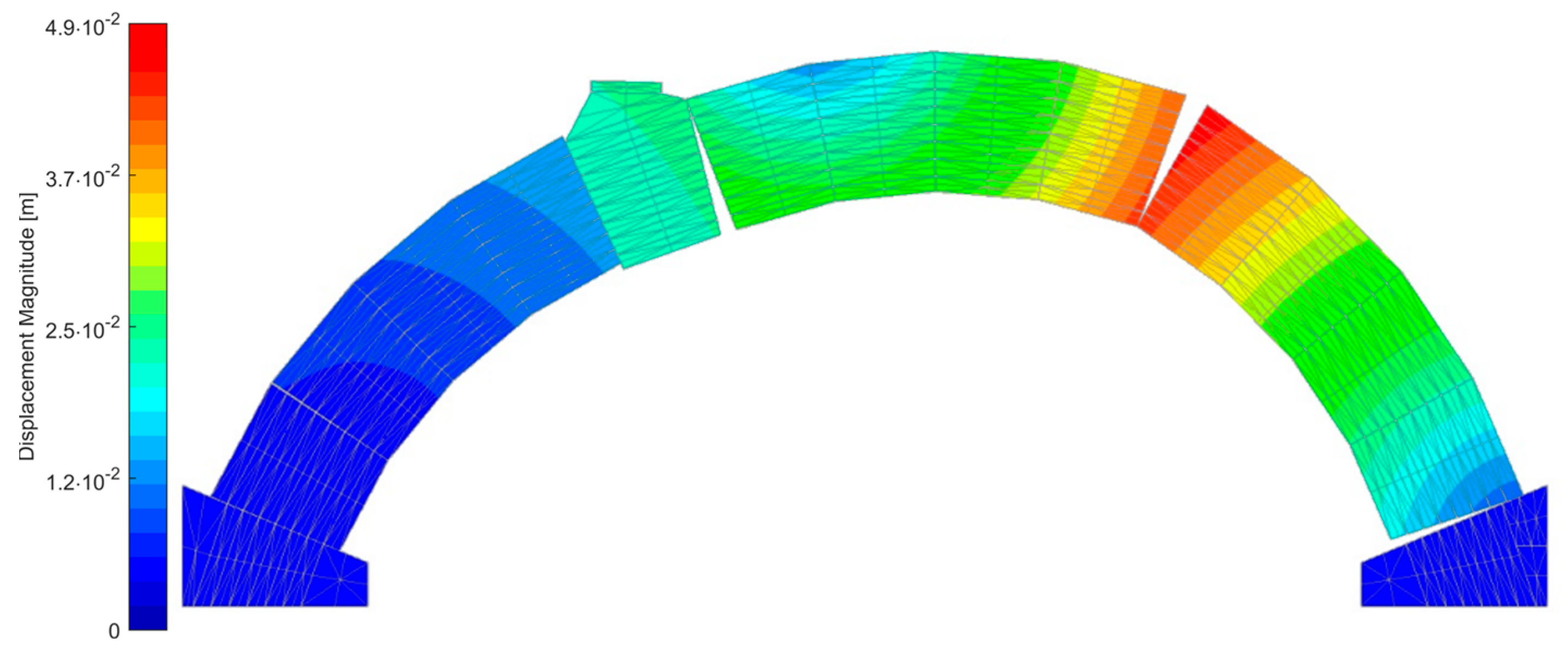
2.3. Discrete Element Modelling of the Quasi-Static Analysis

The physical experimental results observed in [35] were simulated by Pulatsu et al. [32] using 3DEC, a commercial 3D discrete element code developed by Itasca Consulting Group, Inc., Minneapolis, MN, USA.
The discrete elements in 3DEC are of an arbitrary convex polyhedral shape and may either be perfectly rigid or deformable, using a tetrahedral subdivision of their volume. In this study, perfectly rigid elements were applied in a similar way to [32]. In this case, each discrete element had a reference point whose displacements (translations and rotations) during a small finite Δt time interval were calculated using Newton’s laws of motion, taking into consideration the mass and inertia of the element. External forces, such as gravity and contact forces from their neighbours, can act on the elements.
The mechanical model of the contact behaviour fundamentally determines the behaviour of the whole simulated system. The contacts are treated in 3DEC in the following way. The surface of every rigid element is ‘triangulated’, i.e., subdivided into triangles whose nodes are those points where the contact forces are received from the neighbouring elements. This happens to a node when it interpenetrates to the interior of a neighbouring discrete element. Contact deformation is understood to be the relative translation of the node, with respect to its image point on the contact plane, and the same applies to the other contact element as well (see the details in [2,3]). From this deformation, the transmitted force is calculated with the constitutive model of the contact. The contact/joint model is a Mohr–Coulomb model with non-cohesive, frictional contacts (similar to dry contacts in a masonry structure). The following three contact/joint parameters characterise the behaviour of the structure. The normal stiffness expresses how difficult it is to press a node through a neighbouring element face (it is the ratio of compressive force to the depth of interpenetration). The tangential stiffness expresses the resistance against tangential relative translation (it gives the ratio between the increment of tangential relative translation and the increment of transmitted tangential force). Finally, the coefficient of classical Coulomb friction sets the limit to the magnitude of the ratio of tangential force versus compressive force. This study investigates how to efficiently calibrate these three parameters in an automated manner.
An explicit time integration scheme based on central differences is used in 3DEC for simulating the motions over time: the motions caused by a given loading history are achieved by the step-by-step calculation of the displacement increments of the reference points.
Pulatsu et al. [37] and Godio et al. [38] performed sensitivity analysis of different parameters for DEM simulations. Both analysed how the density of surface triangularisation affects the overall stiffness and load-bearing capacity of collections of blocks. The studies showed that for a greater number of contact points with the same contact stiffness a lower value of collapse load is received. If the default two-point discretisation (triangulating a face into 4/8 equal-sized elements using radial or radial-8) of 3DEC is used, then the value of the collapse load is higher. Therefore, in this study, the number of contacts along the joint edge was set to 15.
The normal and shear joint stiffness applied in [32] were calculated based on [39,40]. The joint friction angle ϕ was estimated through reverse engineering. The values used for the micromechanical parameters were kn = 4 GPa/m and ks = 1.6 GPa/m. The initial friction angle was taken as ϕ0 = 30.5°. The ratio of initial friction angle (ϕ0) to residual friction angle (ϕres) was taken as 1 based on [41] to obtain a sliding failure mode (prediction of how the arch will collapse) as with the experimental results. Therefore, the same value was used for the residual friction angle (ϕres).
The quasi-static analysis of a dry-joint masonry arch was performed by applying a vertical displacement rate to the loading plate. The vertical displacement was applied as a fixed velocity to the block. The blocks in the model were rigid and cohesionless, with zero tensile strength. The blocks only had frictional resistance. The support blocks and abutments were fixed in all degrees of freedom and the reaction force was recorded and stored during the analysis. The obtained failure mode (Figure 3) matches the experimental observations (Figure 2).
For the duration of the analysis, displacement was measured at two points:
  • The vertical displacement of the middle of the loading plate shown in Figure 3.
  • The horizontal displacement of the middle of the block at the abutment shown in Figure 3.
The analysis was carried out using the assumptions of both small and large displacements. While the small displacement analysis could not reflect the softening range, the results from the large displacement simulation showed good agreement with the experimental results (Figure 4). Specifically, the large displacement results showed a better fit to the post-peak behaviour, although there was a slight difference between the peak force, but it was almost negligible. Therefore, all the simulations performed in this study were carried out modelling large displacements. Local damping with a value of 0.8 was used in the numerical simulations performed.
A sensitivity analysis carried out in [32] showed the effect of the parameters on the results of the quasi-static loading. They found that the friction angle did not affect the peak strength unless its value was less than 30°. However, it did affect the post-peak behaviour. At the fixed values of kn and ks, described earlier, a complete sliding failure was observed for an interparticle friction angle of 27° and a complete plastic hinge formation was observed for a friction angle of 35°. The experiment showed transitory behaviour: both sliding failure and plastic hinge could be observed. This behaviour was best reproduced in the simulations at a value of 30.5°. The effect of contact stiffnesses on the peak force could not be seen for a fixed friction angle of 30.5° but the displacements obtained for the peak load increased with the decrease in contact stiffness. The post-peak behaviour was influenced by the contact stiffness due to the nonlinear behaviour of dry joint masonry. Therefore, the contact stiffness should be estimated carefully.
In the experiment, the loading velocity was 0.005 mm/s. The computational cost of applying the same loading velocity in the simulations as in the experiment would be extremely high (approximately 1 h for 1 mm/s loading velocity); therefore, using the same velocity for calibration would be inefficient. Sensitivity analysis needs to be carried out to find a trade-off between the accuracy of the analysis and the computational cost (see Section 2.4.2). The main outcome was that, for loading velocities less than or equal to 10 mm/s, the results agreed with those in the experiment, while loading velocities greater than 10 mm/s resulted in unrealistic oscillations or noise in the results. The results in [32] can be replicated with a loading velocity of 5 mm/s but (possibly due to a typing error) the loading velocity mentioned in that paper was 50 mm/s. The values 5 mm/s and 50 mm/s are used interchangeably within their article.
To summarise, the main data of Pulatsu’s 3DEC model were:
  • Element size along the arch thickness (eight blocks): 10 mm;
  • Block material: rigid; eight blocks along the arch thickness (radial direction);
  • Loading velocity: 5 mm/s;
  • Contact stiffness values: kn = 4 GPa/m; ks = 1.6 Gpa/m;
  • Contact friction angle (initial as well as residual): 30.5°.

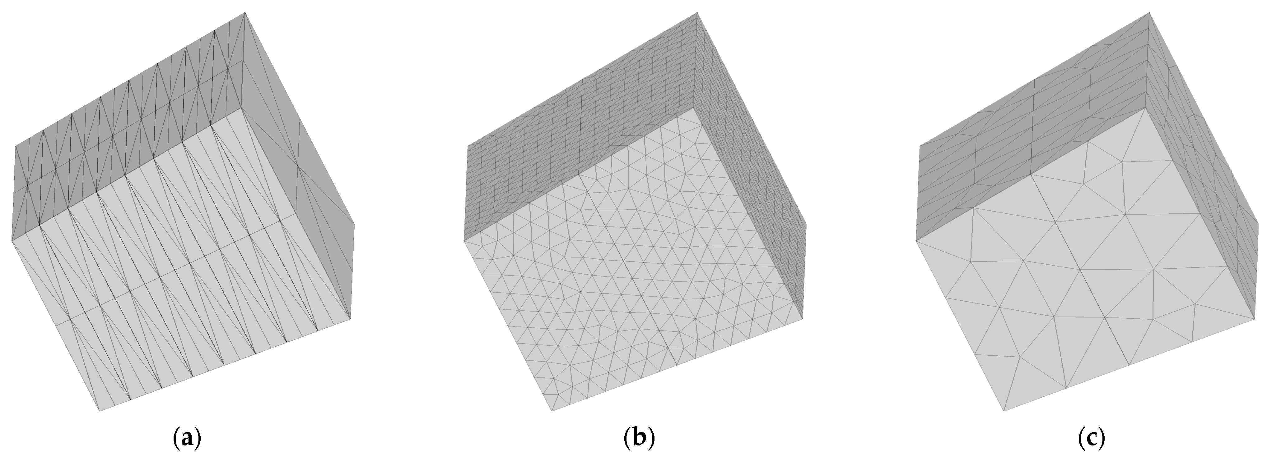
2.4. Modified Surface Discretisation

2.4.1. Introduction

3DEC uses explicit time integration, which means that, even though rather strong artificial damping is used in the simulations, the calculated response oscillates around the exact solution of the problem. This results in unrealistic oscillations of the simulated load–displacement curves around what would be the structural response if infinitely small timesteps could be applied. However, the magnitude of the oscillations can be decreased by reducing timestep length, reducing the velocities in the model and refining the subdivision density of the geometry. In the model made by Pulatsu et al. [32], each stone was made of eight sub-blocks that were clumped (made to be a group of discrete elements adhered together with rigid connections to behave as a single unit) (see Figure 3) to increase the number of contact points and have a sufficiently high resolution of contact mechanics. This is referred to as ‘Pulatsu’s geometry’ hereinafter. 3DEC’s sub-contact method, which sub-divides the faces of the blocks into smaller triangles, offers infinite solutions to segment a geometry. In the case of Pulatsu’s geometry, each face was divided into eight triangles by connecting its centroid with the corners and edge midpoints. The subdivision pattern can have an influence on the mechanical behaviour of the model; hence, a different segmentation was tried as well. In this second type of geometry, each stone was made of only two rigid blocks (see Figure 5) and the triangle mesh was generated algorithmically. Geometries made in this way are called ‘surface meshed geometries’ hereinafter. Figure 6 shows the results of different discretisation techniques on a single stone block: Pulatsu’s and surface meshed geometries with mesh sizes of 12 mm and 35 mm. The necessary mesh density of the modified discrete element model needed to be found in such a way that the results obtained from Pulatsu’s geometry, and those obtained from the surface meshed geometry, become sufficiently close. (The surface meshed geometries were also used to investigate the effect of the surface mesh density on the calibrated parameters.)

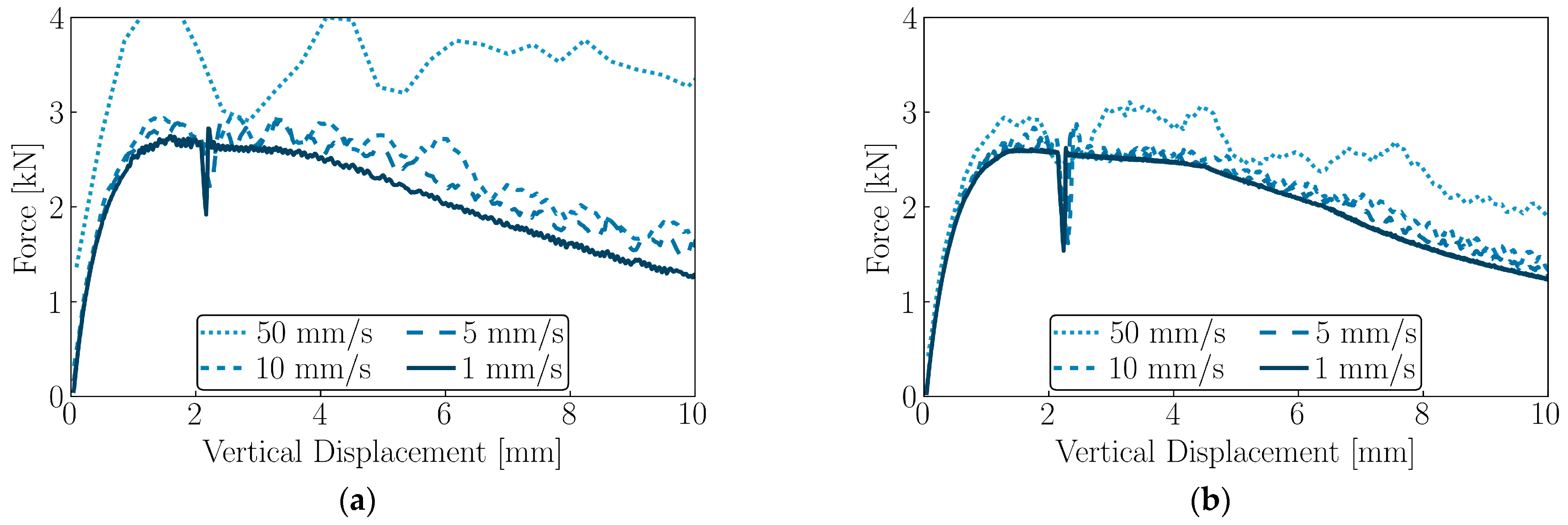
2.4.2. Effect of Loading Velocity

As discussed earlier, the laboratory experiment was carried out by applying very low loading velocity (0.005 mm/s) but, because of the extreme computational costs, in a DEM simulation it was not feasible to use the same loading velocity. Therefore, a compromise was required between the loading velocity and accuracy of the solution. Pulatsu et al. [32] performed a sensitivity analysis for the model and used a loading velocity of 5 mm/s for the results presented in their paper. In this study, a similar sensitivity analysis was undertaken for loading velocities of 1, 5, 10 and 50 mm/s for different types of meshes, as shown in Figure 7. The force–displacement data obtained from simulations with lower loading velocities showed less oscillation. The larger oscillations increased the maximum force obtained.
The loading velocity also affected the stiffness of the structure: lower loading velocity resulted in lower peak force and softer post-peak behaviour. For a 1.6 mm displacement of the loading plateau, the loading force was approximately 16% smaller for 1 mm/s than for 50 mm/s in the case of Pulatsu’s geometry, and the difference became about 35% for the surface meshed geometry. This result suggests that the choice of contact/joint parameters is strongly affected by the loading velocity applied in the simulations. Therefore, calibration has to be carried out for the chosen specific loading velocity. In Figure 7, a good agreement can be seen between the 1 mm/s, 5mm/s and 10 mm/s simulations considering their force–displacement diagram. Reducing the loading velocity results in lower fluctuations, but it also significantly increases computational time. The simulations had to be repeated numerous times in this study; therefore, the calibration was carried out at the highest possible loading velocity, which still provided realistic results; hence, 10 mm/s loading velocity was chosen. The reason for and effect of the sudden drop in force after 2 mm of displacement are discussed in Section 3.4.2.

2.4.3. Effect of Mesh Density

Sensitivity analysis was carried out for each stone made of two blocks. Surface meshes with edge sizes of 10, 12, 15, 20, 25, 30 and 35 mm were created. A good agreement can be seen between the 10 mm, 12 mm and Pulatsu’s element geometry (Figure 8). For 15 mm, the pre-peak response is similar to that of Pulatsu’s element geometry, but the post-peak response is different. Even though the post-peak response is different, the failure mode is similar. For larger mesh sizes, the failure mode is different from that of Pulatsu’s geometry with a loading velocity of 10 mm/s. By reducing the surface mesh size, the accuracy of the solution increases. However, the denser surface mesh increases simulation time as well. A compromise between the accuracy and time required to reach a calibrated set of parameters had to be made without compromising the effectiveness of the solution. Therefore, the 12 mm mesh size was used in the calibration tests in the study.

3. Calibration Methods for the Model Parameters

3.1. Genetic Algorithm

The genetic algorithm (GA) [18] is an evolutionary algorithm inspired by natural selection, which is the process by which a species’ population evolves to adapt to change. The fittest individuals (i.e., those having the lowest values of objective function) survive and produce similar offspring, while weaker individuals start to become extinct over time.
In the genetic algorithm, the ‘population’ refers to a set of solutions participating in the process of optimisation, while the candidate solution to the problem is known as a ‘chromosome’. Each chromosome can contain N genes, which contain the variables to be optimised.
The genetic algorithm consists of a population of chromosomes with genes. The genes store the variables that need to be optimised. The variables in genes can be encoded in different ways, such as binary or value, although binary encoding is more commonly used for its quick crossover and mutation operations. We used real-value encoding, in which the genes are represented by a string of real numbers instead of a string of 1s or 0s, as is the case for binary encoding.
The first step in the genetic algorithm is to replace the existing population by a new population through the selection of suitable parents. The choice of parents is extremely important for the crossover since the new solutions will be from these parents. A variety of methods exist for the selection process. We used fitness proportionate selection, in which each solution is given a probability range based on the value of objective function. As a result, a solution with a lower value of objective function will have a better chance of being selected.
Crossover mimics the reproduction of the natural selection process. The genetic information of two individuals (called ‘parents’) is exchanged to produce two new individuals (called ‘offspring’). There are different methods to perform crossover. We used uniform crossover, in which each gene for an offspring is selected from both parents with a 0.5 probability. If a gene is selected from parent 1, then the gene with the same index is selected from parent 2 for the other offspring.
Mutation allows the introduction of new traits in the genetic information of the offspring. This operator helps to maintain diversity and to make sure that the population does not converge to local optima. We applied random mutation, in which the value of a gene is replaced by a randomly generated value in the search space. In this study, a 10% mutation probability was used.
After the crossover and mutation is completed, the final step is replacing the old population with a new population. The new population is then evaluated by objective function and the process continues until the number of maximum iterations is reached.
In the genetic algorithm, the set of candidate solutions is a population. A population consists of n chromosomes and a chromosome consists of N genes. In this case, N is the number of parameters that need to be calibrated, which are k n , k s and ϕ . The number of chromosomes, which are the set of these parameters, can be chosen freely. For this study, a population of 10 chromosomes were chosen for the genetic algorithm.

3.2. Particle Swarm Optimisation

Particle Swarm Optimisation (PSO) was proposed and developed by Eberhart and Kennedy in 1995. The method was introduced in two papers [33,34]. Particle Swarm Optimisation applies the concept of social interaction to problem solving. It has a profound connection with social relations, concepts and behaviours that emerged from computational study and the simulation of a simplified model of the movement of a swarm of bees or a flock of birds seeking food.
Particle Swarm Optimisation is different from GA, since PSO is a trajectory-based algorithm, i.e., the values are updated by movement in a search space, while the values are updated by the interaction of chromosomes with each other in GA.
Particle Swarm Optimisation is an iterative technique for optimisation, starting with several ‘particles’, whose ‘position vectors’ are the sets of possible values of the parameters to be calibrated. (The coordinates of a particle are the actual values of the parameters.) This collection of particles is known as a swarm of particles. The particles change their ‘positions’ as the values of those parameters to be calibrated gradually change. The value of objective function is calculated for every particle: the actual coordinates (i.e., parameter values) determine how close the force–displacement diagram is to the real experiment (the way in which the value of objective function is determined is described in Section 3.4). In a swarm, each particle knows its best individual position, value of objective function and best global position for the swarm.
For each iteration, the velocity and position of each particle in the swarm are represented by N -dimensional vectors, which are influenced by individual and social knowledge, and this leads to a repeated flight of particles in a solution space to a problem in search of an optimum solution. The velocity of each particle i in a swarm at every iteration of k  is updated according to the following equation [42]:
V k + 1 i = V k i + ϕ 1 R 1 k i p k i x k i + ϕ 2 R 2 k i g k x k i ,
where V k i , x k i are the velocity and position vectors of particle i at iteration step k. R 1 k i and R 2 k i are uniformly distributed N random scalars in the interval of 0–1, each corresponding to a dimension of the particle’s position. p k i is the individual best position of particle i at iteration k and g k is the global best position of the swarm at iteration k. ϕ1 and ϕ2 are called ‘cognitive’ and ‘social’ weights and they act as the weights in the velocity update equation. These values have an influence on how much the individual and global best position affects the velocity and position of the particle. A greater value of cognitive weight encourages exploratory behaviour, i.e., the particle will explore more of the search space, while the social weight encourages exploitative behaviour, meaning that the particles will move towards the best solution already present. Both values influence the optimal solution. If a higher value of the cognitive component is used, the solution may not converge. If a higher value of the social component is used, the solution may converge to a local optimum. In the original algorithm, the values of both the cognitive and social components were taken to be 2. The position of the particle can be updated after calculating the updated velocity [42]:
x k + 1 i = x k i + V k + 1 i .
The initial values of the particle ( x 0 i ) and velocity ( V 0 i ) can be generated randomly or by following any arbitrary rule. In the beginning, the individual best position can be taken as the particle’s own initial position p 0 i = x 0 i .
The global best position of a swarm with n particles is defined as the individual best position of a particle for which the value of objective function is the minimum of individual best positions f p k i of all particles”.
y k { p k 1 , p k 2 , , p k n } | f y ^ k = m i n { f p k 1 , f p k 2 , , f p k n } ,
where yk is the global best position in the entire swarm in an N-dimensional search space.
Particle Swarm Optimisation has gained attention over time, resulting in more and more research being undertaken. The research in [43] has revealed some problems with the original version of PSO, such as entrapment in local optima, performance problems and velocity explosion [34]. Velocity explosion occurs when the value of velocity obtained after each iteration starts to grow towards infinity or extremely large values.
Shi and Eberhart [44] suggested the use of inertia weight ω of a particle. This parameter controls the effect of the particle’s previous velocity on the current velocity. The range of values suggested for ω ∈ [0.9, 1.2].
V k + 1 i = ω V k i + ϕ 1 R 1 k i p k i x k i + ϕ 2 R 2 k i g k x k i .
A relationship between the cognitive component, social component and inertia weight is given by [45]:
ω > 1 2 ϕ 1 + ϕ 2 1 .
The modification of ω can be carried out by using a linear function [46]:
ω k = ω m a x ω m a x ω m i n k m a x k ,
or by using a nonlinear function [47].
ω k = k m a x k m i n k m a x n ω m i n ω m a x + ω m a x ,
where k is the iteration number and k m a x and k m i n are the upper and lower limits of the iterations. In this study, a linear variation for updating ω between 0.8 and 0.4 was used. The value of both the cognitive and social component was taken as being 2, as per the original algorithm. Another suggested modification is the use of a constriction factor [48], which could facilitate faster convergence. The constriction factor K is given by:
K = 2 2 ϕ ϕ 2 4 ϕ
where ϕ = ϕ1 + ϕ2 and ϕ ≥ 4. Equation (4) can be given as:
V k + 1 i = K V k i + ϕ 1 R 1 k i p k i x k i + ϕ 2 R 2 k i g k x k i .
Kar et al. [49] combined the inertia weight and constriction factor. This combination showed improvement in the effectiveness and efficacy of optimisation. The modified form of Equation (1) can be given as:
V k + 1 i = K ω V k i + ϕ 1 R 1 k i p k i x k i + ϕ 2 R 2 k i g k x k i .

3.3. The Novel Method: TBPSO

A distinct feature of the calibration of DEM models is that the evaluation of objective function is computationally very expensive. Hence, an improved version of Particle Swarm Optimisation was introduced to reduce the number of generations/iterations required to reach the optimum solution. The basic principle is that a competent particle (lower value of objective function) will not trust a less competent particle (higher value of objective function) at all. Similarly, if a particle’s competence improves then the trust of the less competent particles in that particle will increase and if a particle’s competence does not improve the trust of the less competent particles in that particle will decrease. The new method was named TBPSO (Trust-Based Particle Optimisation). Note that a different PSO approach already exists with a similar name [50], but it is abbreviated as TMPSO.
In this case, the distance of a particle i to another particle j, d k i j is calculated at step k. Similarly, the distance to all the other particles j = [1…n] is also calculated. Based on the calculated distances, the relative distance d r e l , k i j of a particle i to a particle j is calculated as:
d r e l , k i j = d k i j j = 1 n d k i j .
Then, the trust C k i j of a single particle in other particles is calculated based on the competence of other particles. The competence of a particle can be defined based on its personal best objective function value. The goal is to minimize the value of objective function; therefore, a lower value of objective function means a more competent particle and vice versa. If a particle i’s best objective function value is less than that of particle j, then the trust of particle i in particle j becomes zero. Now, if particle i’s best objective function value is greater than that of particle j, and particle j’s current value of objective function is either equal to its best objective function value or less than the best objective function value of particle j, then the trust of particle i in particle j increases by 1. Similarly, if particle i’s best objective function value is greater than that of particle j, and particle j’s current objective function value is greater than the best objective function value of particle j, then the trust of particle i in particle j decreases by 1.
In summary, a hierarchy is defined for the particles. The most competent particle in the swarm will not trust other particles. Similarly, the least competent particle will trust all other particles. The mathematical representation of the trust calculation is as follows:
0 i f   f p k i f p k j j 1,2 , 3 , , n , C k i j = C k 1 i j + 1 i f   f p k i > f p k j f x k j f p k j j 1,2 , 3 , , n , C k 1 i j 1 i f   f p k i > f p k j f x k j > f p k j j 1,2 , 3 , , n .
The vector difference in position Δ x k i j of each particle to another particle is calculated as:
Δ x k i j = x k i x k j   j 1,2 , 3 , , n .
After calculating the relative distances, trust and difference in vector positions, the velocity can be calculated. The relative distance and trust act as weights for calculating the trust-based velocity component. The component of velocity is calculated based on trust, using the following equation:
T k i = j = 1 n d r e l , k i j C k i j Δ x k i j .
The velocity update equation (Equation (12)) becomes:
V k + 1 i = K ω V k i + ϕ 1 R 1 k i p k i x k i + ϕ 2 R 2 k i g k x k i + ϕ 3 R 3 k i T k i .
In the current case, the parameters ϕ1, ϕ2 and ϕ3 are set to values 1, 1 and 2, respectively. R 3 k i , R 1 k i and R 2 k i , are uniformly distributed N scalars, each corresponding to a dimension of the particle’s position. The weight is updated linearly, in the same way as in PSO.

3.4. Objective Functions

In optimisation problems, the choice of objective function has a significant importance in the accuracy of the optimised values, along with the time taken to converge to a specific value. In problems involving mathematical linear or nonlinear functions and constraints, the evaluated value of an objective function has a direct relation with the variables to be optimised but, in more practical problems (such as the problem of calibrating micromechanical material parameters for DEM simulation), the choice of objective function is greatly limited by the experimental results.
It is also important to note that the change in certain variables might not affect the simulation results at all; therefore, the ‘most impactful’ experimental results need to be present for the calibration with simulation results. In the problem of the calibration of joint parameters for a masonry arch, it cannot be said with surety that a certain experimental result would be sufficient to optimise the material parameters.
The sensitivity analysis carried out in [32] showed that the most important factor in determining the failure mode of the arch is the initial friction angle of the contacts (ϕ0). This also has an impact on peak strength, given that its value is less than 30°. The other most important parameter is the normal contact stiffness kn, which can have a considerable effect on post-peak behaviour. Shear stiffness ks is dependent on normal stiffness, according to [39,40]. The ratio kn/ks is usually set between 2.4 and 2.5 .
The previous calibration attempts, discussed in Section 1, calibrated the parameters to a set of bulk parameters. However, in this case a similar approach cannot be used to calibrate the micromechanical parameters to achieve a “single bulk parameter or multiple bulk parameters”. Instead, the available results are force–displacement diagrams. The displacement data available at two points were shown earlier, in Figure 3. The simulations for calibration were only performed until the maximum vertical displacement of 12 mm and there was no collapse of the arch.
To make use of the available data and the material parameters that need to be calibrated, two different objective functions were used. The loss calculation procedure was the same for both objective functions, but the data obtained from the experiments and the simulations were processed differently. The data used for objective function 1 were raw (i.e., the data are not modified before evaluating the objective function) while, for objective function 2, with the application of the deep neural network (see Section 3.4.2), an approximation of data obtained from both the experiment and simulation was used. By reducing the noise or oscillations in the data, it is the authors’ opinion that the efficiency of the optimisation process can be improved.

3.4.1. Objective Function 1

Objective function 1 uses a sum root squared error between the experimental and simulated force–vertical displacement and force–horizontal displacement diagrams to calculate the fitness value. The additional displacements after the structure was equilibrated for self-weight were taken into account. Therefore, the lower and upper bounds of both vertical and horizontal displacement are set as
w l b = m a x m i n w e x p , m i n w s i m ,
w u b = m i n m a x w e x p , m a x w s i m .
where wexp and wsim are the displacement data from the experimental and simulation data, respectively. wlb and wub are the lower and upper limit set for the displacement, respectively.
Two hundred uniformly distributed points are then generated between the upper and lower bounds of both the vertical and horizontal displacement. Using linear interpolation, the value of force corresponding to each displacement value, for both horizontal and vertical displacements, is calculated. Now, the square root of the sum of the square difference between experimental and simulation data points is calculated for both vertical and horizontal displacements.
f v e r = i F e x p , v e r , i F s i m , v e r , i 2 ,
f h o r = i F e x p , h o r , i F s i m , h o r , i 2 .
where Fexp,ver,i and Fsim,ver,i are interpolated force values for the vertical displacement of the experimental and simulation data. Fexp,hor,i and Fver,hor,i are interpolated force values for the horizontal displacement of the experimental and simulation data. Instead of a multi-objective function optimisation using fver and fhor, a single objective function giving the same weightage to both fver and fhor is used:
f = min f v e r + f h o r .

3.4.2. Objective Function 2

Objective function 1 uses raw experimental and simulation data that contain noise (unrealistic oscillations) to calculate the fitness value. This can cause problems in the calibration process, resulting in being stacked at local optimum values. To avoid this, an artificial neural network model is used in objective function 2 to smooth the graphs of both the experiment and simulation. Figure 9 shows the force–displacement graph of one of the simulations and the effect of different smoothening techniques. It can be seen that the original data along with having oscillations have a drop in force due to the stick-slip phenomenon. Even though the main trend of the curve matches the experimental result well, the fitness value is lower than expected due to the presence of the oscillations and drop.
The oscillations of the force in the force–displacement graphs are directly caused by the numerical errors of the explicit time integration scheme. The numerical result always oscillates around the perfect solution. The precision of the numerical solution can be increased by decreasing the timestep length or the occurring velocities in the model, as seen in Section 2.4.2, where a decrease in loading plate velocity caused a reduction in the oscillation amplitudes. However, such a low loading plate velocity could not be applied, due to the significant increase in simulation time. The sudden drop is caused by a stick-slip phenomenon, which is also a result of the numerical integration. The normal force between the blocks oscillates, which causes the temporary decrease in maximum allowable friction force between the blocks, leading to a sudden slip. The slipping stops when the normal force increases again.
Because oscillations in numerical results are not connected to real physics, they should be disregarded during the analysis of the results, which means that they should not affect the fitness values. The moving average can be helpful in reducing the amplitude of oscillations but cannot eliminate the drop perfectly. To overcome this issue, a neural network is used that can entirely remove the effect of oscillations and drops from the fitness value.
A neural network is based on the biological neural network and tries to mimic its behaviour. Neurons are a group of components or nodes that make up a neural network. These neurons are linked together by a connection known as a synapse. A neuron can communicate a signal or information to another neuron nearby via a synapse. The signal can be received, processed and then passed on to the next neuron by the receiving neuron. The process continues until an output signal is created.
The input xi received by a neuron is multiplied by a corresponding weight wi. The sum of all the products of the weights, with inputs and bias β, is then calculated and passed through an activation/transfer function, which is mostly nonlinear, to produce the output of a neuron. An individual neuron without an activation function is similar to a linear regression problem. Figure 10 shows the illustration of an individual neuron.
A neural network consists of layer(s) of neurons and a layer can consist of a single or multiple neurons. The layers are then connected to each other to make a neural network. Each neural network has an input layer, a hidden layer and an output layer. If the number of hidden layers is greater than 1, then the neural network is referred to as a deep neural network. Figure 11 shows an illustration of a deep neural network.
A neural network learns by modifying the weights and biases after each iteration of the neurons. The weights and biases of neurons are updated based on the loss value, which is the difference between the output produced by the model and expected output. Modification is achieved by using backpropagation, which is a two-step process. The first step is a forward pass in which the output is evaluated for a given input. To update the weights, a backward pass is made, in which the partial derivatives of model parameters (weights and biases) are calculated with respect to loss [51]. The weights and biases are updated to minimise the loss. The process continues until the maximum number of iterations are reached or the loss value falls below a threshold.
A Dense Neural Network was created with five hidden dense layers (each hidden layer containing 20 neurons with a hyperbolic tangent activation function) and the mean absolute error loss function. Loss is minimised using the Adam optimisation algorithm [52]. The force–displacement graphs were discretised into 200 points. Generalisation was not required and all data were used as training data. The same data were used for training for which the final output was needed. There was no need to test the DNN. Each simulation produced two force displacement graphs (one for the vertical and one for the horizontal displacement); hence, two DNNs were trained, one for each graph. Overfitting can cause the DNN to learn the noise instead of learning only the overall trend of the curve. Therefore, it was made sure not to overtrain the DNN. Figure 9 shows that the DNN was able to learn that trend.

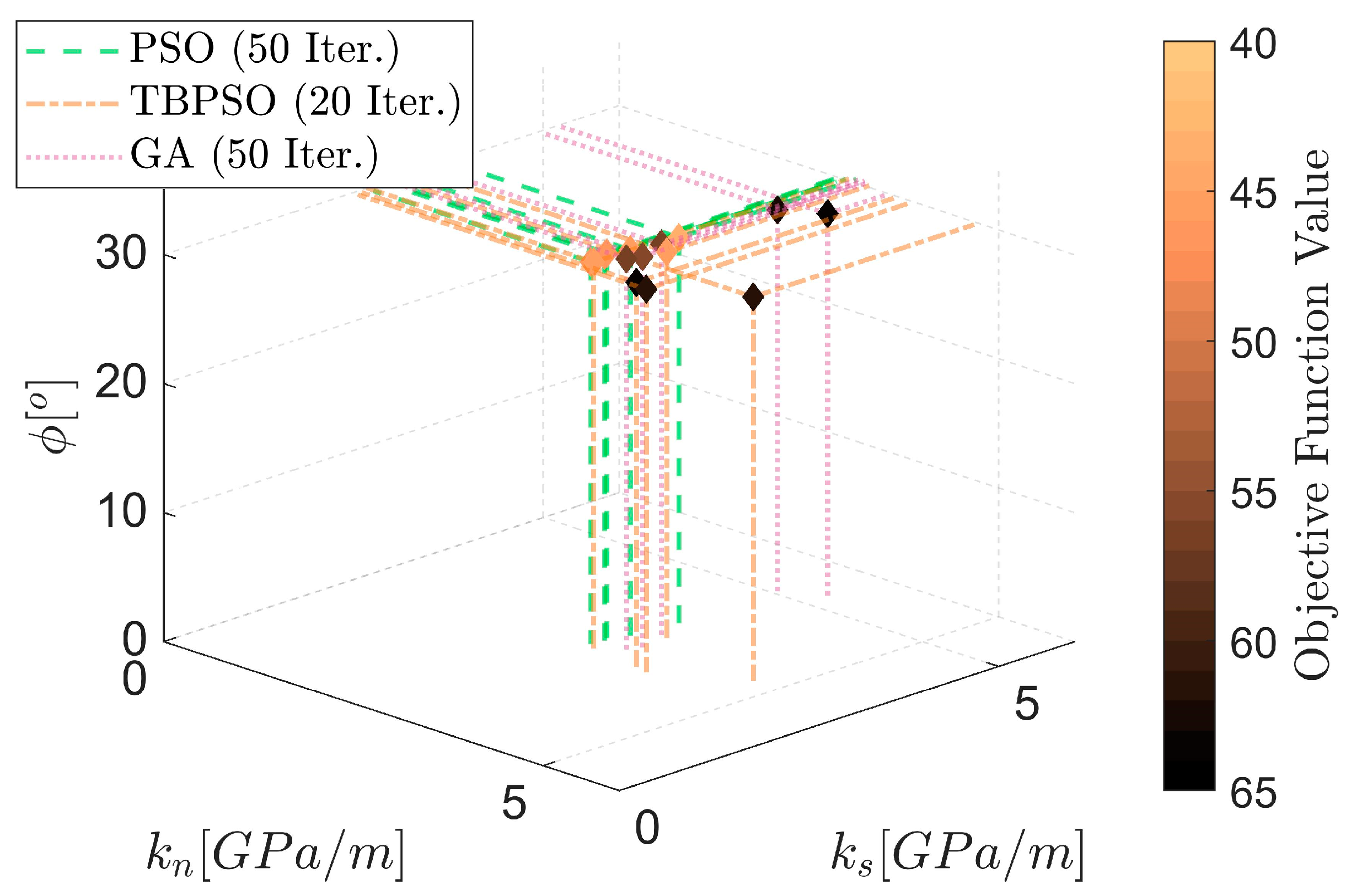
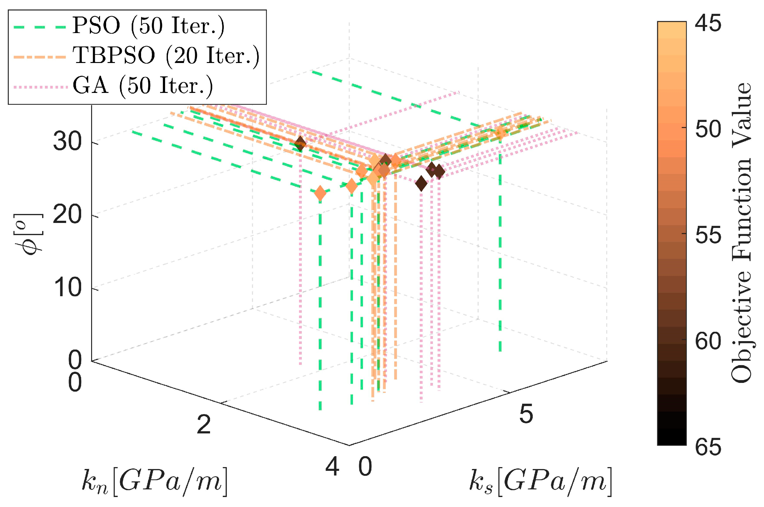
3.4.3. Representation of Objective Function

To give a visual impression of how the micromechanical parameters affect the fit between simulated and real behaviour, a 2D grid with linear spacing is created for normal stiffness and friction angle. The ratio of normal to shear stiffness is taken to be constant, at 2.5. Objective function 1 is evaluated for these parameters and a contour plot is created to show the response of objective function to the change in these parameters. Figure 12 shows that the minimum value of objective function for normal stiffness is between 2 × 10⁹ and 1010, while the friction angle is close to 30°.

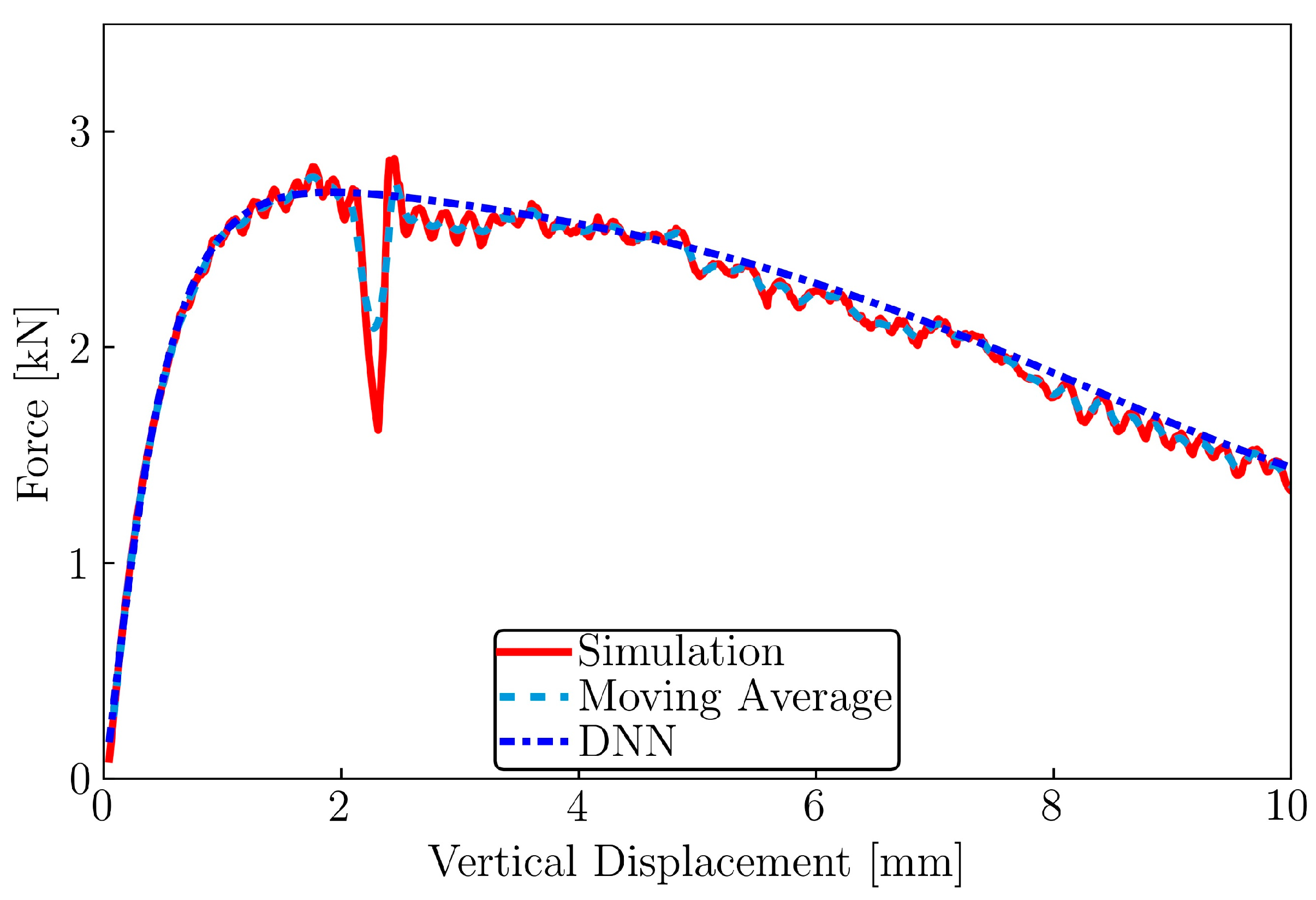
3.5. Software Background and Workflow

The DEM simulations were run in 3DEC and the rest of the calculations were performed using Python. The geneticalgorithm library was used for the GA computations and the neural network was built using TensorFlow. The PSO and TBPSO methods were programmed relying only on the NumPy library. Figure 13 shows the workflow of the calibration process. The calibration started with the random generation of material parameters in Python and the data were then fed to 3DEC. When the simulation was performed, the simulation results were written into a text file. The Python script read this data file and evaluated the objective function. Based on the evaluation of objective function, the values of material parameters were updated and the process was continued until the stopping criteria were reached.

4. Numerical Analysis, Results and Discussion

Pulatsu’s geometry and surface meshed geometry (with 12 mm mesh size) were both calibrated with a 10 mm/s loading velocity. The main aims during the calibration process were to reach an accurate solution and to achieve those results in the minimum number of DEM simulations possible. A simple termination criterion was used for all of the calibrations; the number of iterations/generations had been specified before the beginning of the calibration process.
In order to compare the results objectively, the algorithms were set up in such a way that each iteration would evaluate the objective function exactly ten times, i.e., ten DEM simulations. Therefore, the swarm size for PSO and TBPSO was ten and the number of individuals for GA was also ten. No constraint equations were used in the problem.
The values for normal stiffness, shear stiffness and friction were initially generated from a random uniform distribution. The minimum and maximum values were based on the previous literature and the response of objective function 1 (see Figure 12). The minimum value for kn and ks was set as 108 Pa/m and the maximum value was set as 1010 Pa/m. The minimum and maximum values for friction were set as 25° and 45°, respectively, although, based on the preliminary runs, the maximum and minimum range could have been narrowed down or extended further, but the aim in this study was to achieve the calibrated set of parameters in a given range without having to manually search for the parameters conforming to the experimental behaviour.
To summarise the most important algorithm parameters, a linearly updating weight parameter for both PSO and TBPSO (from 0.8 to 0.4) was used. The values of the cognitive and the social components for PSO were chosen to be 2. For TBPSO, the values used for the cognitive, social and trust components were 1, 1 and 2, respectively. For GA, a uniform crossover with 50% probability and a random mutation with 10% probability were used.
The number of iterations for the basic versions of PSO and GA were first set by running 100 iterations several times. Particle Swarm Optimisation reached an optimum solution after 25–30 iterations (in a few cases), with most of the optimum solutions being reached in 40–50 iterations. For GA, the optimum solution was reached by 40–50 iterations while, in a few cases, it got stuck in local optima and remained in that position for 100 iterations. Since no improvements were seen after 50 iterations, it was decided that PSO and GA would be run for 50 iterations.
Trust-Based Particle Swarm Optimisation was observed to be significantly faster: it reached the optimum solutions obtained in 50–100 iterations by PSO and GA, in 15–20 iterations in most cases.
The number of iterations for PSO, TBPSO and GA were based on the preliminary runs and these settings seemed optimal for both objective functions. Each calibration for a single objective function was carried out at least 10 times due to the stochastic nature of the algorithms. The results for both Pulatsu’s geometry and surface meshed geometry are presented below.
During the calibration process, the approximate runtime of one instance of Pulatsu’s geometry while running 6 threads (6 core/12 thread Intel Core i7-8750-H processor with base frequency of 2.2 GHz, turbo frequency 4.10 Ghz and 16 GB RAM) was between 4 and 6 min. For the surface meshed geometry with mesh size of 12 mm, the average run time on the same configuration was 5 to 8 min. The time demand of the whole calibration can be calculated by determining population/swarm size, the number of necessary iterations and the number simulations that can be run simultaneously.

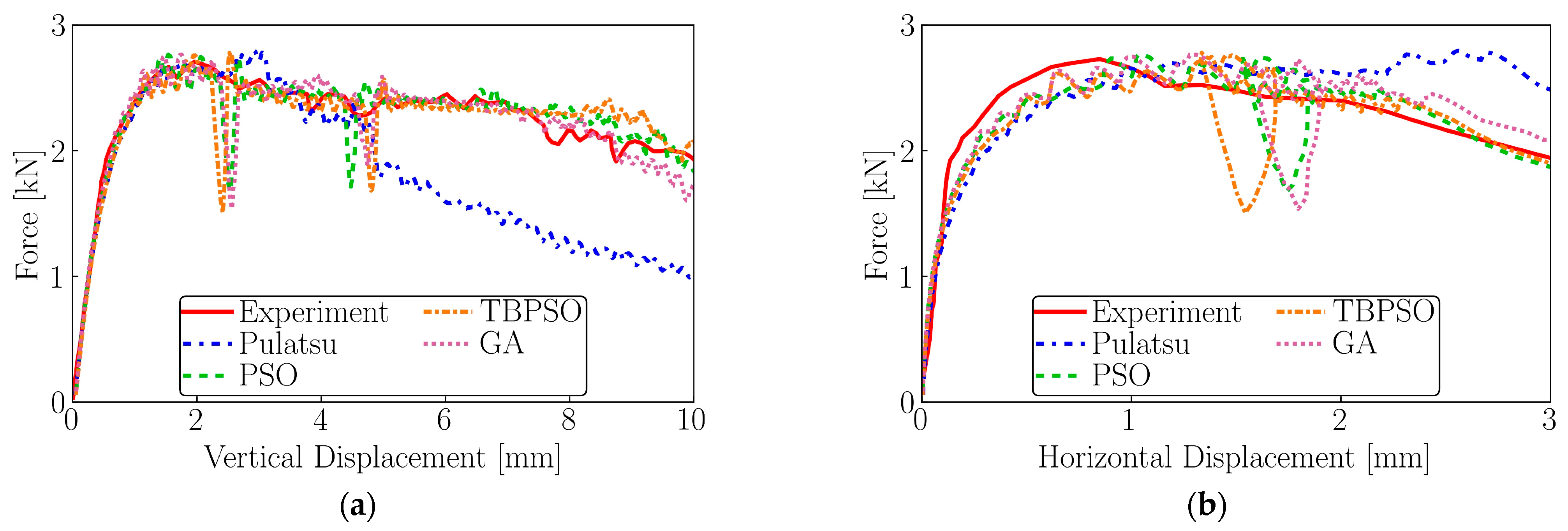
4.1. Pulatsu’s Geometry

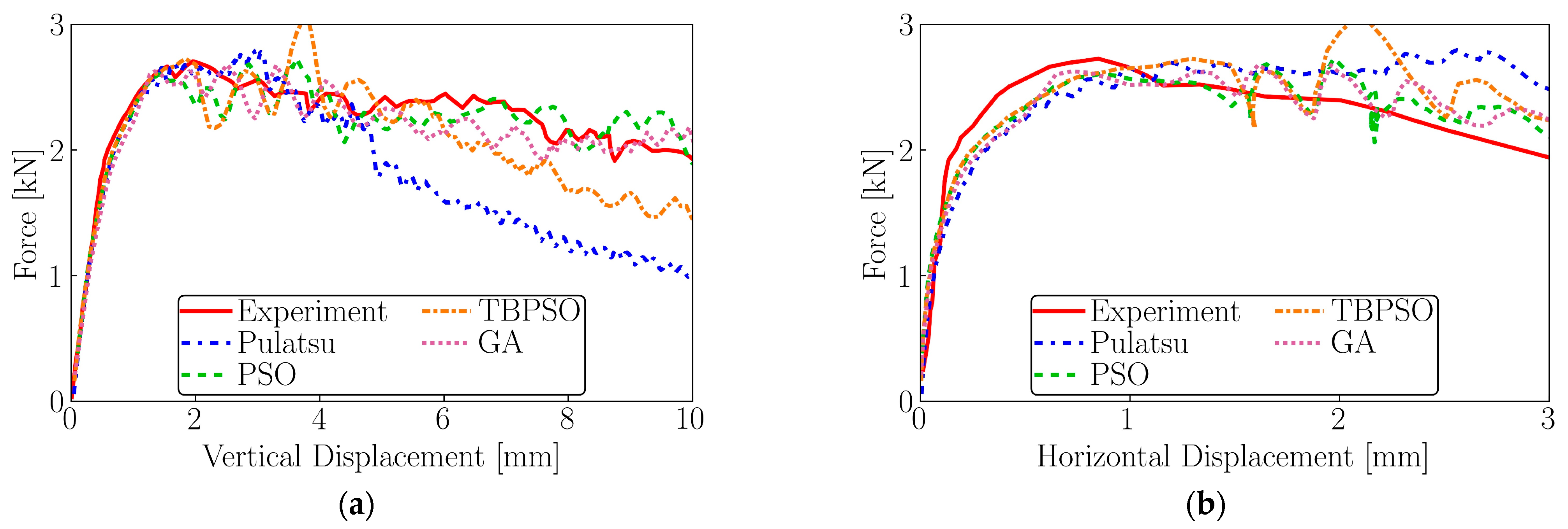
4.1.1. Objective Function 1

Objective function 1 was calculated from raw experimental and simulation data (see Section 3.4.1). Table 1 shows the solution set obtained by PSO and GA after 50 iterations and the solution set obtained after 20 iterations by PSO and TBPSO. Figure 14 presents the five best solution sets obtained from PSO, TBPSO and GA for objective function 1 on Pulatsu’s geometry. It can be seen that most of the values obtained for kn are between 3 and 4 GPa/m except for one case, where it is slightly larger than 4 GPa/m. The value of ks is about the same, except for two cases in which the value is greater than 4 GPa/m. The solutions obtained for ϕ in each set are either close to 30° or above 30°. The best solution was found using 30° by PSO with 50 iterations. There are multiple possible, equally good parameter sets for a single DEM model. Usually, the kn/ks ratio is fixed during manual calibration because the influence of ks is often limited. It was not the case in the automatic calibration; the algorithm could pick any value between the boundaries; therefore, large differences occurred in the kn/ks values between the different parameter sets. It should be noted that GA parameters showed a large scatter in comparison to the other methods.
Figure 15 shows the force versus horizontal and vertical displacement diagrams for the best calibrated set of parameters obtained from objective function 1 for Pulatsu’s geometry. The diagrams show a good agreement with the experiments and also with those obtained from Pulatsu’s parameters, except for the post-peak response in the vertical displacement diagram. The failure mode (three hinges + one sliding surface) with displacement magnitude is shown in Figure 16 and, obtained from these parameters, is similar in Pulatsu’s model and the experiments.

4.1.2. Objective Function 2

Objective function 2 was calculated from smoothed experiment and simulation data (see Section 3.4.2 and Figure 9). Table 2 shows the best solution sets obtained after 50 and 20 iterations. Figure 17 presents the five best solution sets obtained from PSO, TBPSO and GA. The values obtained for kn and ks are similar to the ones obtained from objective function 1. However, in the case of the solutions obtained for ϕ, all the values obtained are equal to or slightly above 30°.
Figure 18 shows the load versus horizontal and vertical load displacement diagrams for the calibrated set of parameters obtained from objective function 2 for Pulatsu’s geometry. An important aspect of using objective function 2 (see Figure 9) is that the friction angle values obtained by this function are consistent. The calibrated parameters gave an improved fit in comparison to those parameters originally applied in [32]. Figure 19 shows the failure mode (three hinges + one sliding surface) is similar to the mode obtained in experiment [35] along with displacement magnitude.

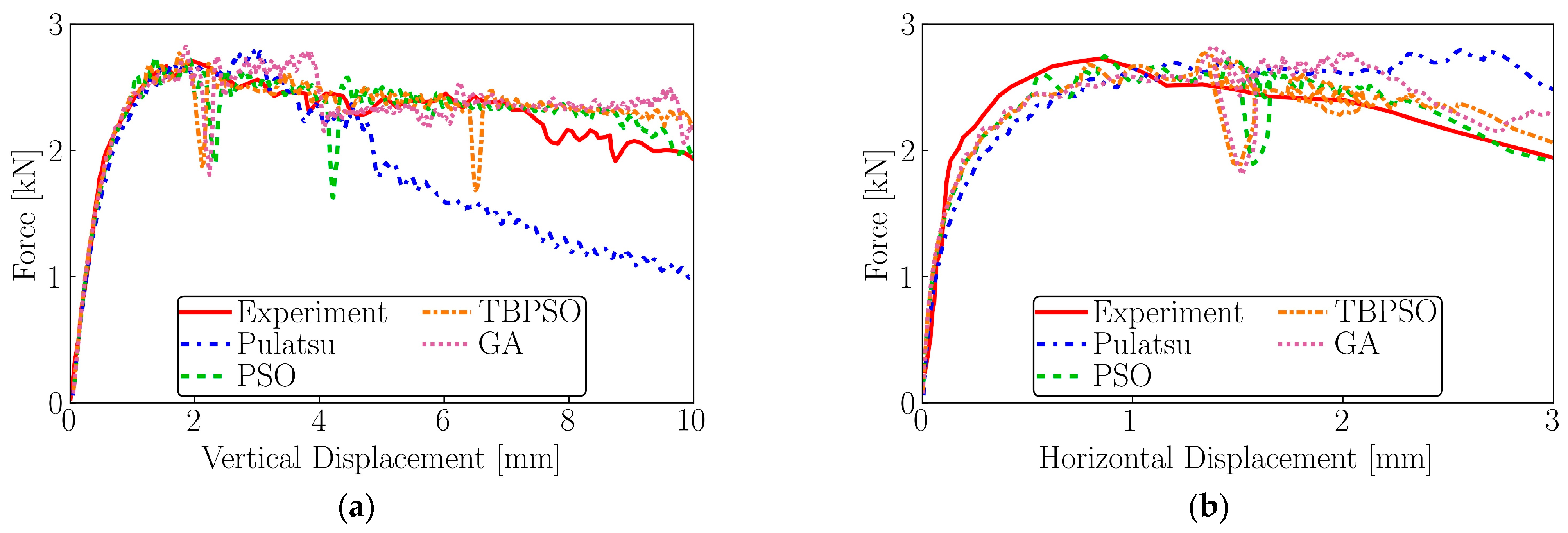
4.2. Surface Densely Meshed Model

A new model with dense surface meshing was also introduced in this study for comparison with Pulatsu’s geometry and to investigate the effect of the subdivision method.

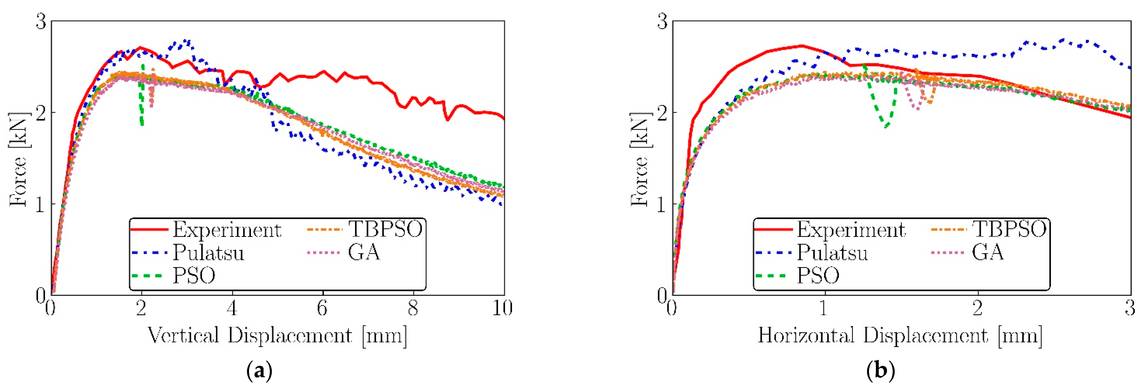
4.2.1. Objective Function 1

Table 3 presents the solution set obtained from PSO and GA after 50 iterations and the solution sets obtained from PSO and TBPSO after 20 iterations. Figure 20 presents the five best solution sets obtained from the PSO, TBPSO and GA for objective function 1 and a densely meshed model. The values obtained for kn are similar to the values used in [32]. The value of k s is, however, rather scattered between 2 and 4 GPa/m, which suggests that the mechanical behaviour is not very sensitive to the value of ks. The value of ϕ is mostly calibrated above 30° but, in some cases, it is calibrated to values less than 30°. It should be noted that all of the methods lead to results with a large scatter, presumably due to the oscillating nature of the force–displacement behaviour.
In the force displacement diagrams shown in Figure 21, the dark lines denoted as ‘Pulatsu’ show the simulation results given by the original Pulatsu model (geometry as well as material parameters) without automated calibration. It can be seen that the results gained with the surface densely meshed model and automated calibration closely match the results from Pulatsu’s geometry and parameter set. The difference between the Pulatsu model and surface densely meshed model is the higher noise levels in the simulation data obtained from the densely meshed model. The post-peak behaviour shown in the experiment is better captured by the models using automatic calibration than by the original material parameter set in [32]. The failure mode obtained (three hinges + one sliding surface) from the best set of parameters is shown in Figure 22 and agrees with what was seen in the experiment [35].

4.2.2. Objective Function 2

The calibrated materials obtained from objective function 2 are very similar to the values obtained previously, as can be seen in Table 4. Most of the values of kn, ks obtained are close to 3 GPa/m and most of the values of ϕ are also above 30°. The calibrated parameters obtained are shown in Figure 23.
The force displacement diagrams shown in Figure 24 are similar to the previously obtained diagrams, showing a greater level of noise and a downward trend, which is in agreement with the experimental results and better captured by the models using automatically calibrated material parameters than by the original parameter set in [32]. The scatter of the alternative calibrated parameter sets (Figure 24) is smaller for objective function 2 than for objective function 1 (Figure 20), particularly the TBPSO results, which became less scattered. Figure 25 presents a similar failure mode (three hinges + one sliding surface) as observed in experiment [35].
The automated calibration procedure performed better in matching the load displacement curves obtained by the experiments and the parameter sets obtained from the calibration procedures shown in Figure 15, Figure 18, Figure 21 and Figure 24 (compared to the load displacement curves obtained from the parameter set used in [32]). The failure modes (three hinges + one sliding surface) shown in Figure 16, Figure 19, Figure 22 and Figure 25 are also in line with the experiment and with the outcome from the parameter set applied in [32].

4.2.3. Reduced Loading Plate Velocity

The velocity of the loading plate was 5·10−3 mm/s in the experiment and 10 mm/s in the simulations, which is a significant difference. The calibration procedure could not be performed with a smaller velocity in reasonable time and it was discussed in Section 2.4.2 that realistic behaviour could be computed with 10 mm/s as well. However, verification simulations could be run with smaller speeds. Figure 26 shows the results of simulations with a loading velocity of 0.5 mm/s using the surface meshed geometry and calibrated parameters with objective function 2. A decrease in the amplitude of numeric oscillations is clearly visible. The post-peak force also decreased in the case of the algorithmically calibrated parameters and became similar to Pulatsu’s original parameters. The decrease in force agrees with the observation made in Section 2.4.2 that lower loading velocity results in lower peak force and softer post-peak behaviour.

5. Conclusions

With the preparatory investigations carried out at the beginning of this study, it was found that the load–displacement behaviour of the DEM models of masonry arches is very sensitive to the velocity of (displacement-controlled) loading. Before starting the calibration, a necessary step would be to carefully select both mesh density and loading velocity for use in the simulations. These values are usually a compromise between accuracy and computational time. By the careful selection of these two values, a considerable amount of time can be saved during the calibration process while preserving accuracy.
In the main part of this study, three different algorithms were employed for the purpose of the calibration of a masonry arch. The reason for the choice of PSO and GA was that these are well established methods and work efficiently on a variety of real-world problems. The choice of algorithm can affect the efficiency and accuracy of the calibration process. However, it should also be kept in mind that no optimization algorithm is best for every problem [53]. The main aim is not only to automate the calibration process but also to find a speedy method where the number of iterations (i.e., the number of necessary simulations of the loading process) is low. Seeing best solution sets obtained from the PSO and GA after 50 iterations in Section 4.1 and Section 4.2 (see Table 1, Table 2, Table 3 and Table 4), it can be said that, although PSO and GA were both run for 50 iterations, the PSO leads to significantly better results (lower values of objective function). From the solution sets obtained after 20 iterations by PSO and TBPSO (see Table 1, Table 2, Table 3 and Table 4), it can be seen that the TBPSO reaches a better match of simulation and experimental results than PSO. In some cases, contrarily to TBPSO, PSO did not converge after 20 iterations, leading to higher values of objective function. Based on this, it can be concluded that TBPSO performs better than PSO in the current problem. It can also be concluded that PSO performs better than GA.
We recommend using PSO, TBPSO and perhaps other improved forms of PSO instead of GA, due to faster convergence to a better solution. However, the calibration process is highly dependent on the parameters controlling the optimisation process. These parameters (which control the behaviour of optimisation algorithms, such as weight parameters in PSO, mutation probabilities in GA, etc.) can be changed and, in turn, affect the optimisation process. The tuning of such parameters is very important. Therefore, it should be noted that changing the parameters used in this study might improve the performance of GA, perhaps even making it comparable with PSO and TBPSO. Further investigations are required in future.
The calibration process could also be improved by the presence of additional load displacement diagrams. The reason for this is that, by tracking the motion of more points of the structure, the behaviour of the whole structure would be better captured and, hence, a better set of calibrated parameters produced. Any point of the structure can be tracked in the simulation software but in real experiments the number of sensors is usually limited. Therefore, the placement of sensors during laboratory testing has to be performed strategically, so as to capture complete structural behaviour. In the current case, the load displacement data are only available for two points and both of those points are utilised in calibration, while the failure mode is used for validating the results.
It is hard to obtain detailed experimental data about the mechanical behaviour of masonry structures. Because historical buildings cannot be tested, assumptions are often made regarding their mechanical parameters. For the same reason, experiments are often conducted with structures that represent a typical class of masonry structure or a typical failure mode. Even when in possession of experimental data, it is still a challenge to calibrate the numerical models. The introduced method offers a tool to automatise and accelerate this calibration process and to increase the chance of finding the optimal parameter values.

Author Contributions

Conceptualization, K.B. and J.B.; Methodology, G.K., J.B. and K.B.; Software, G.K. and Á.O.; Formal Analysis, G.K.; Investigation, G.K. and Á.O.; Resources, Á.O. and K.B.; Writing—Original Draft Preparation, G.K. and K.B.; Writing—Review and Editing, Á.O.; Visualization, G.K.; Supervision, K.B. and J.B.; Funding Acquisition, K.B. and Á.O. All authors have read and agreed to the published version of the manuscript.

Funding

Support by the Hungarian National Science Fund under the OTKA K-138642 grant is gratefully acknowledged. The research reported in this paper is part of project no. BME-NVA-02, implemented with the support provided by the Ministry of Innovation and Technology of Hungary from the National Research, Development and Innovation Fund, financed under the TKP2021 funding scheme.

Institutional Review Board Statement

Not applicable.

Informed Consent Statement

Not applicable.

Data Availability Statement

The data presented in this study are available upon request from the corresponding author.

Acknowledgments

The authors express their gratitude to Itasca Consulting Group Inc. for providing the full version of 3DEC software under the frame of the Itasca Educational Partnership (IEP) Research Program. We would like to thank the support of Fabian Dedecker, Matthew Purvance and Sacha Emam regarding the use and technical background of 3DEC software. Special thanks to Bora Pulatsu for kindly providing the 3DEC command files of his original simulations.

Conflicts of Interest

The authors declare no conflict of interest.

References

  1. Cundall, P.A. A computer model for simulating progressive, large scale movement in blocky rock systems. In Proceedings of the International Symposium on Rock Mechanics, Nancy, France, 4–6 October 1971; Volume 2. [Google Scholar]
  2. Sarhosis, V.; Bagi, K.; Lemos, J.V.; Milani, G. Computational Modeling of Masonry Structures Using the Discrete Element Method; IGI Global: Hershey, PA, USA, 2016. [Google Scholar] [CrossRef]
  3. Sarhosis, V.; Lemos, J.V.; Bagi, K. Discrete element modeling. In Numerical Modeling of Masonry and Historical Structures; Elsevier: Amsterdam, The Netherlands, 2019; pp. 469–501. [Google Scholar] [CrossRef]
  4. Munjiza, A. The Combined Finite-Discrete Element Method, 1st ed.; Wiley: Oxford, UK, 2004. [Google Scholar] [CrossRef]
  5. Munjiza, A.; Galić, M.; Smoljanović, H.; Marović, P.; Mihanović, A.; Živaljić, N.; Williams, J.; Avital, E. Aspects of the hybrid finite discrete element simulation technology in science and engineering. Int. J. Eng. Model. 2020, 32, 45–55. [Google Scholar] [CrossRef]
  6. Coetzee, C.J. Review: Calibration of the discrete element method. Powder Technol. 2017, 310, 104–142. [Google Scholar] [CrossRef]
  7. Yoon, J. Application of experimental design and optimization to PFC model calibration in uniaxial compression simulation. Int. J. Rock Mech. Min. Sci. 2007, 44, 871–889. [Google Scholar] [CrossRef]
  8. Rackl, M.; Hanley, K.J. A methodical calibration procedure for discrete element models. Powder Technol. 2017, 307, 73–83. [Google Scholar] [CrossRef] [Green Version]
  9. Ben Turkia, S.; Wilke, D.N.; Pizette, P.; Govender, N.; Abriak, N.-E. Benefits of virtual calibration for discrete element parameter estimation from bulk experiments. Granul. Matter 2019, 21, 110. [Google Scholar] [CrossRef]
  10. Zeng, H.; Xu, W.; Zang, M.; Yang, P.; Guo, X. Calibration and validation of DEM-FEM model parameters using upscaled particles based on physical experiments and simulations. Adv. Powder Technol. 2020, 31, 3947–3959. [Google Scholar] [CrossRef]
  11. Bhalode, P.; Ierapetritou, M. Discrete element modeling for continuous powder feeding operation: Calibration and system analysis. Int. J. Pharm. 2020, 585, 119427. [Google Scholar] [CrossRef]
  12. Mohajeri, M.J.; van Rhee, C.; Schott, D.L. Replicating cohesive and stress-history-dependent behavior of bulk solids: Feasibility and definiteness in DEM calibration procedure. Adv. Powder Technol. 2021, 32, 1532–1548. [Google Scholar] [CrossRef]
  13. Cressie, N.A.C. Spatial Prediction and Kriging. In Statistics for Spatial Data; John Wiley & Sons, Inc.: Hoboken, NJ, USA, 2015; pp. 105–209. [Google Scholar] [CrossRef]
  14. Benvenuti, L.; Kloss, C.; Pirker, S. Identification of DEM simulation parameters by Artificial Neural Networks and bulk experiments. Powder Technol. 2016, 291, 456–465. [Google Scholar] [CrossRef]
  15. Westbrink, F.; Elbel, A.; Schwung, A.; Ding, S.X. Optimization of DEM parameters using multi-objective reinforcement learning. Powder Technol. 2020, 379, 602–616. [Google Scholar] [CrossRef]
  16. Do, H.Q.; Aragón, A.M.; Schott, D.L. A calibration framework for discrete element model parameters using genetic algorithms. Adv. Powder Technol. 2018, 29, 1393–1403. [Google Scholar] [CrossRef]
  17. Mohajeri, M.J.; Do, H.Q.; Schott, D.L. DEM calibration of cohesive material in the ring shear test by applying a genetic algorithm framework. Adv. Powder Technol. 2020, 31, 1838–1850. [Google Scholar] [CrossRef]
  18. Holland, J.H. Adaptation in Natural and Artificial Systems: An Introductory Analysis with Applications to Biology, Control, and Artificial Intelligence; 1st MIT Press, Ed.; MIT Press: Cambridge, MA, USA, 1992. [Google Scholar]
  19. Sarhosis, V. Optimisation procedure for material parameter identification for masonry constitutive models. Int. J. Mason. Res. Innov. 2016, 1, 48–58. [Google Scholar] [CrossRef]
  20. Goodfellow, I.; Bengio, Y.; Courville, A. Deep Learning; The MIT Press: Cambridge, MA, USA, 2016. [Google Scholar]
  21. D’Altri, A.M.; Sarhosis, V.; Milani, G.; Rots, J.; Cattari, S.; Lagomarsino, S.; Sacco, E.; Tralli, A.; Castellazzi, G.; de Miranda, S. Modeling Strategies for the Computational Analysis of Unreinforced Masonry Structures: Review and Classification. Arch. Comput. Methods Eng. 2020, 27, 1153–1185. [Google Scholar] [CrossRef]
  22. Heyman, J. The stone skeleton. Int. J. Solids Struct. 1966, 2, 249–279. [Google Scholar] [CrossRef]
  23. Bagi, K. When Heyman’s Safe Theorem of rigid block systems fails: Non-Heymanian collapse modes of masonry structures. Int. J. Solids Struct. 2014, 51, 2696–2705. [Google Scholar] [CrossRef] [Green Version]
  24. Block, P.; Ochsendorf, J. Thrust Network Analysis: A New Methodology for 3D Equilibrium. J. Int. Assoc. Shell Spat. Struct. 2007, 48, 167–173. [Google Scholar]
  25. Chiozzi, A.; Milani, G.; Tralli, A. A Genetic Algorithm NURBS-based new approach for fast kinematic limit analysis of masonry vaults. Comput. Struct. 2017, 182, 187–204. [Google Scholar] [CrossRef]
  26. Nela, B.; Rios, A.J.; Pingaro, M.; Reccia, E.; Trovalusci, P. Masonry Arches Simulations Using Cohesion Parameter as Code Enrichment for Limit Analysis Approach. Int. J. Mason. Res. Innov. 2022, in press. [Google Scholar] [CrossRef]
  27. Nela, B.; Rios, A.J.; Pingaro, M.; Reccia, E.; Trovalusci, P. Limit analysis of locally reinforced masonry arches. Eng. Struct. 2022, 271, 114921. [Google Scholar] [CrossRef]
  28. Sinopoli, A.; Rapallini, M.; Smars, P. Plasticity, Coulomb Friction and Sliding in the Limit Analysis of Masonry Arches. In Proceedings of the 4th International Conference on Arch Bridges (ARCH’04), Barcelona, Spain, 17–19 November 2004. [Google Scholar]
  29. Gilbert, M.; Casapulla, C.; Ahmed, H.M. Limit analysis of masonry block structures with non-associative frictional joints using linear programming. Comput. Struct. 2006, 84, 873–887. [Google Scholar] [CrossRef]
  30. Casapulla, C.; Argiento, L.U. In-plane frictional resistances in dry block masonry walls and rocking-sliding failure modes revisited and experimentally validated. Compos. Part B Eng. 2018, 132, 197–213. [Google Scholar] [CrossRef]
  31. Pepe, M.; Pingaro, M.; Trovalusci, P.; Reccia, E.; Leonetti, L. Micromodels for the in-plane failure analysis of masonry walls: Limit Analysis, FEM and FEM/DEM approaches. Frat. E Integrità Strutt. 2019, 14, 504–516. [Google Scholar] [CrossRef] [Green Version]
  32. Pulatsu, B.; Gonen, S.; Zonno, G. Static and Impact Response of a Single-Span Stone Masonry Arch. Infrastructures 2021, 6, 178. [Google Scholar] [CrossRef]
  33. Eberhart, R.C.; Kennedy, J. A new optimizer using particle swarm theory. In Proceedings of the MHS’95 Sixth International Symposium on Micro Machine and Human Science, Nagoya, Japan, 4–6 October 1995. [Google Scholar] [CrossRef]
  34. Kennedy, J.; Eberhart, R.C. Particle swarm optimization. Swarm Intell. 1995, 1, 33–57. [Google Scholar] [CrossRef]
  35. Birhane, T.H. Blast Analysis of Railway Masonry Bridges. M.Sc. Thesis, University of Minho, Braga, Portugal, 2009. [Google Scholar]
  36. Vasconcelos, G. Experimental Investigations on the Mechanics of Stone Masonry: Characterization of Granites and Behavior of Ancient Masonry Shear Walls. Ph.D. Thesis, University of Minho, Braga, Portugal, 2005. [Google Scholar]
  37. Pulatsu, B.; Bretas, E.M.; Lourenco, P.B. Discrete element modeling of masonry structures: Validation and application. Earthq. Struct. 2016, 11, 563–582. [Google Scholar] [CrossRef]
  38. Godio, M.; Stefanou, I.; Sab, K. Effects of the dilatancy of joints and of the size of the building blocks on the mechanical behavior of masonry structures. Meccanica 2018, 53, 1629–1643. [Google Scholar] [CrossRef]
  39. Lourenço, P.B.; Oliveira, D.V.; Roca, P.; Orduña, A. Dry Joint Stone Masonry Walls Subjected to In-Plane Combined Loading. J. Struct. Eng. 2005, 131, 1665–1673. [Google Scholar] [CrossRef] [Green Version]
  40. Pulatsu, B.; Gonen, S.; Erdogmus, E.; Lourenço, P.B.; Lemos, J.V.; Prakash, R. In-plane structural performance of dry-joint stone masonry Walls: A spatial and non-spatial stochastic discontinuum analysis. Eng. Struct. 2021, 242, 112620. [Google Scholar] [CrossRef]
  41. Lourenço, P.B.; Ramos, L.F. Characterization of Cyclic Behavior of Dry Masonry Joints. J. Struct. Eng. 2004, 130, 779–786. [Google Scholar] [CrossRef]
  42. Reza, B.M.; Zbigniew, M. Particle Swarm Optimization for Single Objective Continuous Space Problems: A Review. Evol Comput. 2017, 25, 1–54. [Google Scholar] [CrossRef]
  43. Clerc, M.; Kennedy, J. The particle swarm—Explosion, stability, and convergence in a multidimensional complex space. IEEE Trans. Evol. Comput. 2002, 6, 58–73. [Google Scholar] [CrossRef] [Green Version]
  44. Shi, Y.H.; Eberhart, R. A modified particle swarm optimizer. In Proceedings of the 1998 IEEE International Conference on Evolutionary Computation Proceedings IEEE World Congress on Computational Intelligence (Cat No98TH8360), Anchorage, AK, USA, 4–9 May 1998. [Google Scholar] [CrossRef]
  45. Bergh, F.V.D. An Analysis of Particle Swarm Optimizers. Ph.D. Thesis, University of Pretoria, Pretoria, South Africa, 2002. [Google Scholar]
  46. Eberhart, R.C.; Shi, Y. Comparing inertia weights and constriction factors in particle swarm optimization. In Proceedings of the 2000 Congress on Evolutionary Computation CEC00 (Cat No00TH8512), La Jolla, CA, USA, 16–19 July 2000. [Google Scholar] [CrossRef]
  47. Chatterjee, A.; Siarry, P. Nonlinear inertia weight variation for dynamic adaptation in particle swarm optimization. Comput. Oper. Res. 2006, 33, 859–871. [Google Scholar] [CrossRef]
  48. Clerc, M. The swarm and the queen: Towards a deterministic and adaptive particle swarm optimization. In Proceedings of the 1999 Congress on Evolutionary Computation-CEC99 (Cat No 99TH8406), Washington, DC, USA, 6–9 July 1999. [Google Scholar] [CrossRef]
  49. Kar, R.; Mandal, D.; Bardhan, S.; Ghoshal, S.P. Optimization of linear phase FIR band pass filter using Particle Swarm Optimization with Constriction Factor and Inertia Weight Approach. In Proceedings of the 2011 IEEE Symposium on Industrial Electronics and Applications, Langkawi, Malaysia, 25–28 September 2011. [Google Scholar] [CrossRef]
  50. Huang, W.M.; Deng, Z.R.; Li, R.H.; Tang, X.X. Trust-Based Particle Swarm Optimization for Grid Task Scheduling. Appl. Mech. Mater. 2012, 239–240, 1331–1335. [Google Scholar] [CrossRef]
  51. Deng, L. Deep Learning: Methods and Applications. Found. Trends Signal Process 2013, 7, 197–387. [Google Scholar] [CrossRef] [Green Version]
  52. Kingma, D.P.; Ba, J. Adam: A Method for Stochastic Optimization. arXiv 2014, arXiv:1412.6980. [Google Scholar] [CrossRef]
  53. Wolpert, D.H.; Macready, W.G. No free lunch theorems for optimization. IEEE Trans. Evol. Comput. 1997, 1, 67–82. [Google Scholar] [CrossRef] [Green Version]
Figure 1. Masonry Stone Arch Prototype Quasi-Static Experiment, reproduced from [35].
Infrastructures 08 00064 g001
Figure 2. Deformed arch shape at the ultimate displacement (12 mm), reproduced from [35].
Infrastructures 08 00064 g002
Figure 3. Discrete elements and the failure mode (plastic hinges and sliding failure) from DEM, reproduced from [32].
Infrastructures 08 00064 g003
Figure 4. Load–displacement curves of experiment and DEM model for small and large displacements: (a) vertical displacement, (b) horizontal displacement, reproduced from [32].
Infrastructures 08 00064 g004
Figure 5. Discrete elements of the surface meshed geometries (with two blocks along the radial thickness).
Infrastructures 08 00064 g005
Figure 6. Meshing of: (a) Pulatsu’s geometry, (b) surface meshed geometry with mesh size of 12 mm, (c) surface meshed geometry with mesh size of 35 mm.
Infrastructures 08 00064 g006
Figure 7. Velocity sensitivity results for (a) Pulatsu’s geometry and for (b) the 12 mm surface mesh.
Infrastructures 08 00064 g007
Figure 8. Mesh sensitivity for 10 mm/s loading velocity (the sudden drop of the force post-peak indicates the ‘stick-slip’ phenomenon).
Infrastructures 08 00064 g008
Figure 9. Comparison of simulation, moving average and dense neural network (DNN) force–vertical displacement diagram.
Infrastructures 08 00064 g009
Figure 10. Illustration of an individual neuron.
Infrastructures 08 00064 g010
Figure 11. Illustration of a Deep Neural Network.
Infrastructures 08 00064 g011
Figure 12. Fitness values for varying interparticle friction ϕ (°) and normal stiffness kn (Pa/m) parameters calculated by Objective Function 1.
Infrastructures 08 00064 g012
Figure 13. Workflow of the calibration process.
Infrastructures 08 00064 g013
Figure 14. Position of calibrated material parameters of Pulatsu’s geometry (objective function 1 PSO and GA: 50 iterations; TBPSO: 20 iterations).
Infrastructures 08 00064 g014
Figure 15. Best calibrated material parameter load displacement diagrams of Pulatsu’s geometry (objective function 1, PSO and GA: 50 iterations; TBPSO: 20 iterations); (a) vertical displacement, (b) horizontal displacement.
Infrastructures 08 00064 g015
Figure 16. Failure mode of Pulatsu’s geometry for best set of material parameters using objective function 1; the colour legend represents the displacements in metres.
Infrastructures 08 00064 g016
Figure 17. Position of calibrated material parameters of Pulatsu’s geometry (objective function 2, PSO and GA: 50 iterations; TBPSO: 20 iterations).
Infrastructures 08 00064 g017
Figure 18. Calibrated material parameter load displacement diagrams of Pulatsu’s geometry (objective function 2, PSO and GA: 50 iterations; TBPSO: 20 iterations): (a) vertical displacement, (b) horizontal displacement.
Infrastructures 08 00064 g018
Figure 19. Failure mode of Pulatsu’s geometry for best set of material parameters using objective function 2; the colour legend represents the displacements in metres.
Infrastructures 08 00064 g019
Figure 20. Position of calibrated material parameters of densely meshed geometry (objective function 1, PSO and GA: 50 iterations; TBPSO: 20 iterations).
Infrastructures 08 00064 g020
Figure 21. Calibrated material parameter load displacement diagrams of densely meshed geometry (objective function 1, PSO and GA: 50 iterations; TBPSO: 20 iterations): (a) vertical displacement, (b) horizontal displacement.
Infrastructures 08 00064 g021
Figure 22. Failure mode of densely meshed geometry for best set of material parameters using objective function 1; the colour legend represents the displacements in metres.
Infrastructures 08 00064 g022
Figure 23. Position of calibrated material parameters of densely meshed geometry (objective function 2, PSO and GA: 50 iterations; TBPSO: 20 iterations).
Infrastructures 08 00064 g023
Figure 24. Calibrated material parameter load displacement diagrams of densely meshed geometry (objective function 2, PSO and GA: 50 iterations; TBPSO: 20 iterations): (a) vertical displacement, (b) horizontal displacement.
Infrastructures 08 00064 g024
Figure 25. Failure mode of densely meshed geometry for best set of material parameters using objective function 2; the colour legend represents the displacements in metres.
Infrastructures 08 00064 g025
Figure 26. Load displacement diagrams of the surface meshed geometry using calibrated parameters with objective function 2 at reduced (5 × 10⁻⁴ m/s) loading plate velocity: (a) vertical displacement, (b) horizontal displacement.
Infrastructures 08 00064 g026
Table 1. Five best solution sets for objective function 1 of Pulatsu’s geometry.
Calibration
Process
Number of IterationsRun IDkn (GPa/m)ks (GPa/m)ϕ (°)Fitness (-)
PSO5013.133.6630.3143.4
22.993.1630.0545.9
32.892.9229.8946.0
42.872.7629.6346.7
52.852.9929.8346.9
GA5013.303.0130.4055.0
23.203.3630.5056.0
33.242.8630.4056.3
43.095.0029.8062.0
53.535.2229.9063.0
PSO2014.171.1729.6763.3
24.021.4429.8363.7
34.421.0029.7864.9
43.092.5434.6882.4
53.243.4739.1185.0
TBPSO2013.032.6430.1645.4
23.303.3330.1545.8
33.802.5629.7061.1
44.683.0929.7861.9
53.622.6129.7963.1
Table 2. Five best solution sets for objective function 2 of Pulatsu’s geometry.
Calibration ProcessNumber of IterationsRun IDkn (GPa/m)ks (GPa/m)ϕ (°)Fitness (-)
PSO5013.183.5830.1943.4
23.343.2630.2744.9
33.242.7030.2345.9
43.403.4930.2546.1
53.372.8030.3246.3
GA5013.136.6830.243.9
23.054.1530.247.7
32.444.3530.054.9
43.385.7330.160.2
52.542.9730.163.7
PSO2013.902.3830.5560.0
23.403.1529.9761.0
32.931.9530.0863.1
45.300.8229.7865.5
53.201.6936.4090.2
TBPSO2013.313.3730.1843.8
23.223.2130.3045.5
33.423.6330.4550.5
43.402.2930.4153.4
53.562.1030.3556.9
Table 3. Five best solution sets for objective function 1 of densely meshed geometry.
Calibration ProcessNumber of IterationsRun IDkn (Gpa/m)ks (Gpa/m)ϕ (°)Fitness (-)
PSO5013.112.2230.2057.3
22.924.4630.3361.4
32.821.5529.7661.7
42.705.7930.0361.9
53.891.5429.9763.9
GA5013.403.9930.0059.9
23.543.1630.0060.4
33.757.1230.2064.6
43.103.6130.4066.5
53.033.9529.6066.8
PSO2013.273.3330.0166.0
27.000.9428.7867.9
36.760.5128.5368.9
42.113.2337.38108.2
52.492.4536.71112.4
TBPSO2012.926.2030.2056.3
23.563.4729.6861.2
33.582.6530.1063.4
43.194.4430.0064.2
53.251.7829.6665.7
Table 4. Five best solution sets for objective function 2 of densely meshed geometry.
Calibration ProcessNumber of IterationsRun IDkn (GPa/m)ks (GPa/m)ϕ (°)Fitness (-)
PSO5012.996.7130.1948.1
23.071.9430.0449.0
32.812.7730.1349.1
42.982.9530.2350.0
52.941.2229.7450.5
GA5012.793.5530.3157.4
21.713.0630.3059.1
33.244.0829.7059.4
43.403.9930.0059.9
53.543.1630.0060.4
PSO2016.780.5629.6457.5
24.660.6229.6158.1
34.962.6929.4563.2
42.432.8436.4971.7
53.670.2529.32110.7
TBPSO2013.142.4530.5046.7
22.683.4430.2147.4
32.843.7630.1850.4
43.023.0530.4352.2
52.972.9830.4854.9
Disclaimer/Publisher’s Note: The statements, opinions and data contained in all publications are solely those of the individual author(s) and contributor(s) and not of MDPI and/or the editor(s). MDPI and/or the editor(s) disclaim responsibility for any injury to people or property resulting from any ideas, methods, instructions or products referred to in the content.

