


A Space Fractional Uphill Dispersion in Traffic Flow Model with Solutions by the Trial Equation Method


Abstract
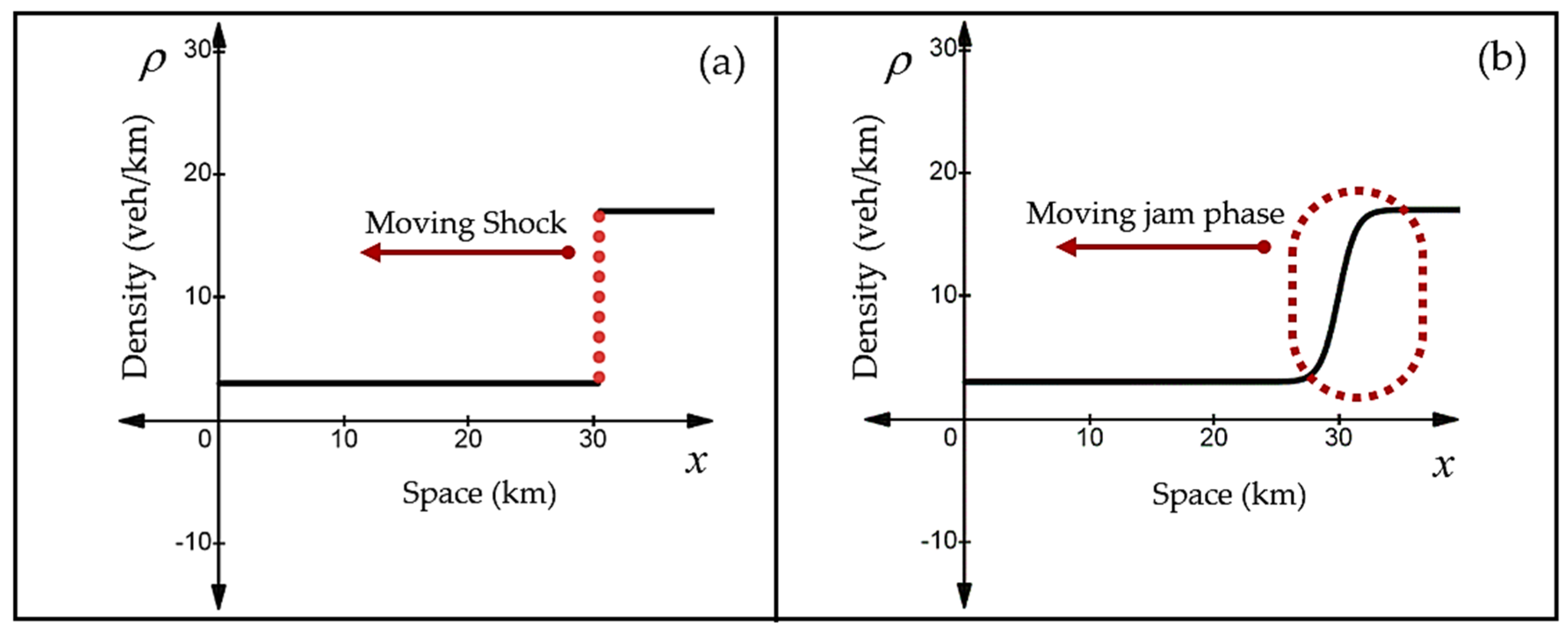
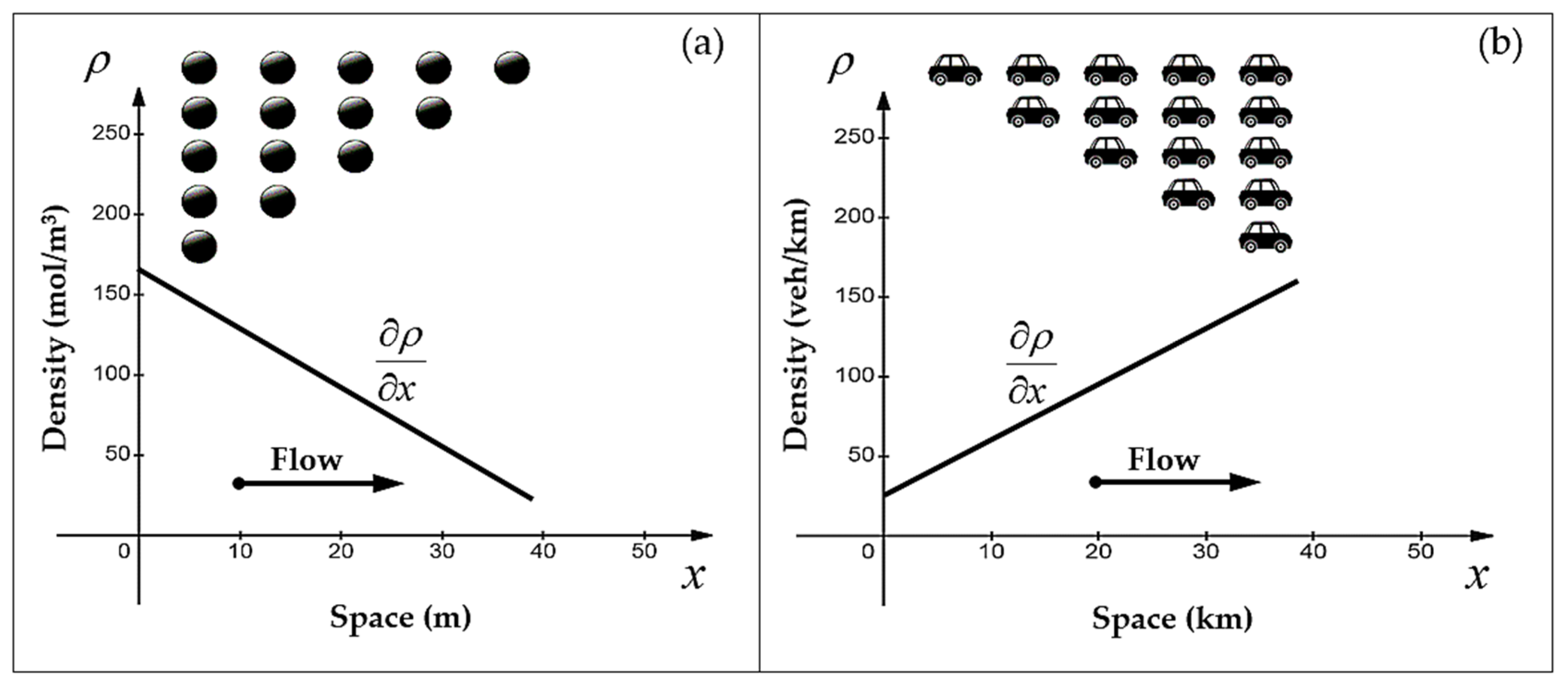
:1. Introduction
2. Proposed Methodology
2.1. The GFFD Fractional Derivative
2.2. Outline of the Trial Equation Method
- Step 1. Using the fractional transformation,where , are nonzero constant. Equation (6) is then converted to a nonlinear ordinary differential equation as,where is a polynomial of and its derivatives and the notation denotes the derivative with respect to .
- Step 2. Suppose the trial equation is of the form,where and are all constant and . N and M are positive integers which can be determined by balancing the linear term of the highest order with the highest order of nonlinear term, whereas and are polynomials of . Placing Equation (9) into Equation (8) precedes an equation of polynomial of as follows,
- Step 3. Setting the coefficients to zero yields a system of algebraic equations concerning the unknowns , , and Then, we solve this system to determine the values of and with the help of symbolic computation software such as Maple 2021.
- Step 4. Rewrite Equation (9) in the classical integral form as,where is a constant to be determined later. Applying the complete discrimination system for the polynomial , we can know the number and multiplicities of the distinct real roots of polynomial . Finally, by solving the infinite integral Equation (11) the exact solutions of Equation (6) will be derived.
3. Problem Formulation
4. Solutions
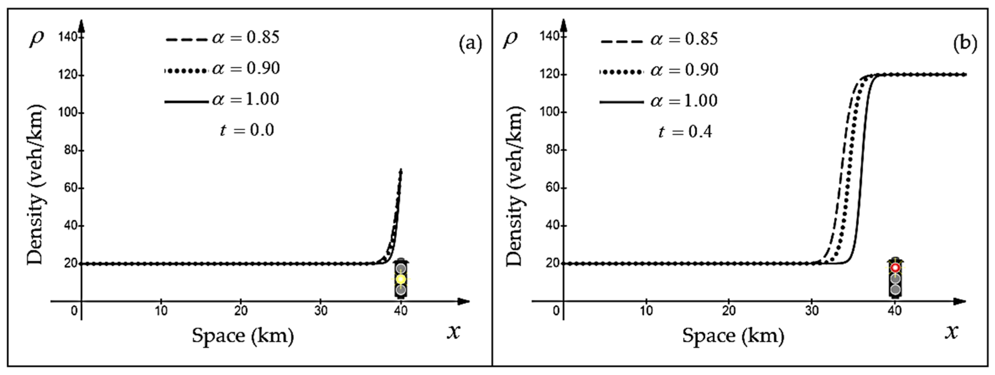
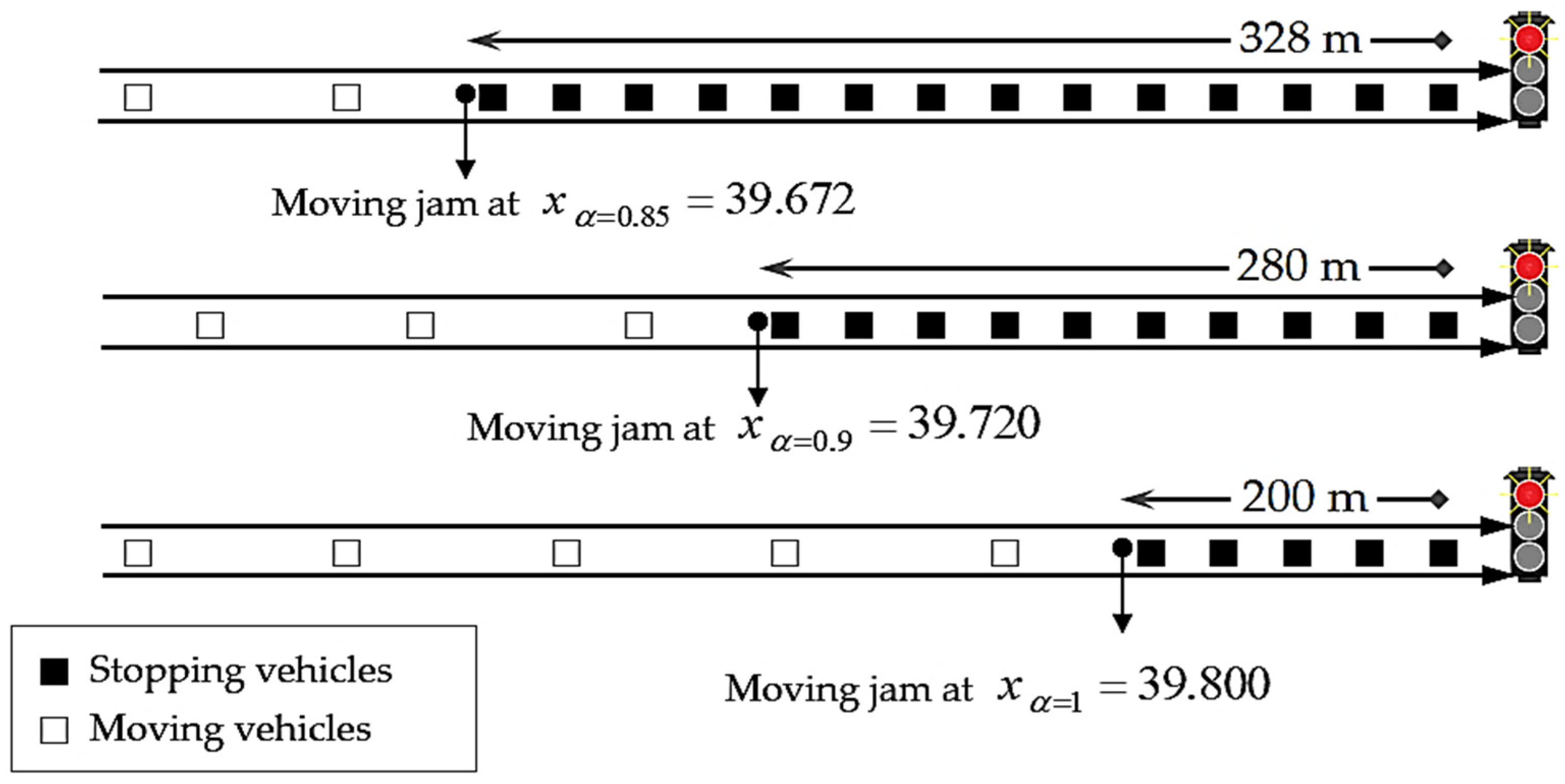
5. Simulation
6. Conclusions
Author Contributions
Funding
Data Availability Statement
Conflicts of Interest
References
- Lighthill, M.J.; Whitham, G.B. On kinematic waves-II. A theory of traffic flow on long crowded roads. Proc. R. Soc. Lond. Ser. A Math. Phys. Sci. 1955, 229, 317–345. [Google Scholar]
- Richards, P.I. Shock waves on the highway. Oper. Res. 1956, 4, 42–51. [Google Scholar] [CrossRef]
- Kuhne, R.; Michalopoulos, P. Continuum Flow Models. In Traffic Flow Theory: A State of the Art Report Revised Monograph on Traffic Flow Theory; Oak Ridge National Laboratory: Oak Ridge, TN, USA, 1997. [Google Scholar]
- Ketcheson, D.I.; LeVeque, R.J.; del Razo, M.J. Riemann Problems and Jupyter Solutions; SIAM: Philadelphia, PA, USA, 2020. [Google Scholar]
- Jafaripournimchahi, A.; Cai, Y.; Wang, H.; Sun, L.; Tang, Y.; Babadi, A.A. A viscous continuum traffic flow model based on the cooperative car-following behaviour of connected and autonomous vehicles. IET Intell. Transp. Syst. 2022, 2022, 1–19. [Google Scholar] [CrossRef]
- Payne, H.J. Models of freeway traffic and control. In Mathematical Models of Public Systems; Simulation Council: Raleigh, NC, USA, 1971; Volume 1, pp. 51–61. [Google Scholar]
- Whitham, G.B. Linear and Nonlinear Waves; Wiley: New York, NY, USA, 1974. [Google Scholar]
- Zhang, H. A theory of non-equilibrium traffic flow. Transp. Res. Part B Methodol. 1998, 32, 485–498. [Google Scholar] [CrossRef]
- Foy, L.R. Steady state solutions of hyperbolic systems of conservation laws with viscosity terms. Comm. Pure Appl. Math. 1964, 17, 177–188. [Google Scholar] [CrossRef]
- Yu, L.; Li, T.; Shi, Z.K. The effect of diffusion in a new viscous continuum traffic model. Phys. Lett. A 2010, 374, 2346–2355. [Google Scholar] [CrossRef]
- Aw, A.; Rascle, M. Resurrection of “second order” models of traffic flow. SIAM J. Appl. Math. 2000, 60, 916–938. [Google Scholar] [CrossRef] [Green Version]
- Richardson, A.D. Refined Macroscopic Traffic Modelling via Systems of Conservation Laws. Master’s Thesis, Department of Mathematics and Statistics, University of Victoria, Victoria, BC, Canada, 2012. [Google Scholar]
- Daganzo, C.F. Requiem for second-order fluid approximations of traffic flow. Transp. Res. Part B Methodol. 1995, 29, 277–286. [Google Scholar] [CrossRef]
- Li, J.; Chen, Q.Y.; Wang, H.; Ni, D. Analysis of LWR model with fundamental diagram subject to uncertainties. Transportmetrica 2012, 8, 387–405. [Google Scholar] [CrossRef]
- Rosini, M.D. Non-equilibrium Traffic Models. In Macroscopic Models for Vehicular Flows and Crowd Dynamics: Theory and Applications; Understanding Complex Systems; Springer: Berlin/Heidelberg, Germany, 2013; pp. 175–190. [Google Scholar]
- Matveev, L.V. Anomalous nonequilibrium transport simulations using a model of statistically homogeneous fractured-porous medium. Phys. A Stat. Mech. Appl. 2014, 406, 119–130. [Google Scholar] [CrossRef]
- Peter, O.J.; Shaikh, A.S.; Ibrahim, M.O.; Nisar, K.S.; Baleanu, D.; Khan, I.; Abioye, A.I. Analysis and dynamics of fractional order mathematical model of COVID-19 in Nigeria using atangana-baleanu operator. Comput. Mater. Contin. 2021, 66, 1823–1848. [Google Scholar] [CrossRef]
- Agrawal, K.; Kumar, R.; Kumar, S.; Hadid, S.; Momani, S. Bernoulli wavelet method for non-linear fractional Glucose–Insulin regulatory dynamical system. Chaos Solitons Fract. 2022, 164, 112632. [Google Scholar] [CrossRef]
- Acay, B.; Bas, E.; Abdeljawad, T. Fractional economic models based on market equilibrium in the frame of different type kernels. Chaos Solitons Fract. 2020, 130, 109438. [Google Scholar] [CrossRef]
- Podlubny, I. Fractional Differential Equations; Academic Press: San Diego, CA, USA, 1999; ISBN 0-1255-8840-2. [Google Scholar]
- Phang, C.; Ismail, N.F.; Isah, A.; Loh, J.R. A new efficient numerical scheme for solving fractional optimal control problems via a Genocchi operational matrix of integration. J. Vib. Control 2018, 24, 3036–3048. [Google Scholar] [CrossRef]
- Alzabut, J.; Selvam, A.G.M.; Dhineshbabu, R.; Tyagi, S.; Ghaderi, M.; Rezapour, S. A Caputo discrete fractional-order thermostat model with one and two sensors fractional boundary conditions depending on positive parameters by using the Lipschitz-type inequality. J. Inequal. Appl. 2022, 2022, 56. [Google Scholar] [CrossRef]
- Fomin, S.; Chugunov, V.; Hashida, T. The effect of non-Fickian diffusion for modelling the anomalous diffusion of contaminant from fracture into porous rock matrix with bordering alteration zone. Transp. Por. Media 2010, 81, 187–205. [Google Scholar] [CrossRef]
- Wheatcraft, S.W.; Meerschaert, M.M. Fractional conservation of mass. Adv. Water Resour. 2008, 31, 1377–1381. [Google Scholar] [CrossRef]
- Li, T. L1 stability of conservation laws for a traffic flow model. Electron. J. Differ. Equ. 2001, 2001, 1–18. [Google Scholar]
- Ishola, C.; Taiwo, O.; Adebisi, A.; Peter, O.J. Numerical solution of two-dimensional Fredholm integro-differential equations by Chebyshev integral operational matrix method. J. Appl. Math. Comput. Mech. 2022, 21, 29–40. [Google Scholar] [CrossRef]
- Peter, O.J. Transmission dynamics of fractional order Brucellosis model using Caputo–Fabrizio operator. Int. J. Differ. Equ. 2020, 2020, 2791380. [Google Scholar] [CrossRef]
- Wu, G.C. A fractional variational iteration method for solving fractional nonlinear differential equations. Comput. Math. Appl. 2011, 61, 2186–2190. [Google Scholar] [CrossRef] [Green Version]
- Adebisi, A.F.; Ojurongbe, T.A.; Okunlola, K.A.; Peter, O.J. Application of Chebyshev polynomial basis function on the solution of Volterra integro-differential equations using Galerkin method. Math. Comput. Sci. 2021, 2, 41–51. [Google Scholar]
- Sonmezoglu, A. Exact solutions for some fractional differential equations. Adv. Math. Phys. 2015, 2015, 567842. [Google Scholar] [CrossRef] [Green Version]
- Aderyani, S.R.; Saadati, R.; Vahidi, J.; Allahviranloo, T. The exact solutions of the conformable time-fractional modified nonlinear Schrödinger equation by the Trial equation method and modified Trial equation method. Adv. Math. Phys. 2022, 2022, 4318192. [Google Scholar] [CrossRef]
- Martínez, F.; Kaabar, K.A. A Novel theoretical investigation of the Abu-Shady–Kaabar fractional derivative as a modeling tool for science and engineering. Comput. Math. Methods Med. 2022, 2022, 4119082. [Google Scholar] [CrossRef]
- Abu-Shady, M.; Kaabar, K.A. A Generalized definition of the fractional derivative with applications. Math. Probl. Eng. 2021, 2021, 9444803. [Google Scholar] [CrossRef]
- Bulut, H.; Baskonus, H.M.; Pandir, Y. The modified trial equation method for fractional wave equation and time fractional generalized Burgers equation. Abstr. Appl. Anal. 2013, 2013, 636802. [Google Scholar] [CrossRef]
- Holmes, M.H. Texts in applied mathematics 56. In Introduction to the Foundations of Applied Mathematics; Springer Science and Business Media: Berlin, Germany, 2009. [Google Scholar]
- Gartner, N.H.; Messer, C.J.; Rathi, A.K. Revised Monograph on Traffic Flow Theory: A State-of-the-Art Report; National Transportation Library: Washington, DC, USA, 2001.
- Callister, W.D.; Rethwisch, D.G. Materials Science and Engineering, 8th ed.; John Wiley and Sons: Hoboken, NJ, USA, 2019. [Google Scholar]
- Colangeli, M.; De Masi, A.; Presutti, E. Microscopic models for uphill diffusion. J. Phys. A Math. Theor. 2017, 50, 435002. [Google Scholar] [CrossRef]
- Krishna, R. Uphill diffusion in multicomponent mixtures. J. Chem. Soc. Rev. 2015, 44, 2812–2836. [Google Scholar] [CrossRef] [Green Version]
- Meerschaert, M.M.; Zhang, Y.; Baeumer, B. Tempered anomalous diffusion in heterogeneous systems. Geophys. Res. Lett. 2008, 35, L17403. [Google Scholar] [CrossRef]
- Cartea, Á.; del Castillo-Negrete, D. Fluid limit of the continuous-time random walk with general Lévy jump distribution functions. Phys. Rev. E 2007, 76, 041105. [Google Scholar] [CrossRef] [Green Version]
- Metzler, R.; Klafter, J. The random walk’s guide to anomalous diffusion: A fractional dynamics approach. Phys. Rep. 2000, 339, 1–77. [Google Scholar] [CrossRef]
- Schumer, R.; Benson, D.A.; Meerschaert, M.M.; Wheatcraft, S.W. Eulerian derivation of the fractional advection–dispersion equation. J. Contam. Hydrol. 2001, 48, 69–88. [Google Scholar] [CrossRef]
- Kochubei, A.N. Fractional-order diffusion. Differ. Equ. 1990, 26, 485–492. [Google Scholar]
- Greenshields, B.D. A study of traffic capacity. In Proceedings of the Fourteenth Annual Meeting of the Highway Research Board, Washington, DC, USA, 6–7 December 1934; pp. 448–477. Available online: http://pubsindex.trb.org/view.aspx?id=120649 (accessed on 8 June 2022).
- Kumar, D.; Tchier, F.; Singh, J.; Baleanu, D. An efficient computational technique for fractal vehicular traffic flow. Entropy 2018, 20, 259. [Google Scholar] [CrossRef] [Green Version]
- Yang, X.J.; Machado, J.A.T.; Baleanu, D. On exact traveling-wave solutions for local fractional Korteweg-de Vries equation. Chaos Interdiscip. J. Nonlinear Sci. 2016, 26, 084312. [Google Scholar] [CrossRef]
- Wang, L.F.; Yang, X.J.; Baleanu, D.; Cattani, C.; Zhao, Y. Fractal dynamical model of vehicular traffic flow within the local fractional conservation laws. Abstr. Appl. Anal. 2014, 2014, 635760. [Google Scholar] [CrossRef] [Green Version]
- Jassim, H.K. On approximate methods for fractal vehicular traffic flow. TWMS J. App. Eng. Math. 2017, 7, 58–65. [Google Scholar]
- Singh, N.; Kumar, K.; Goswami, P.; Jafari, H. Analytical method to solve the local fractional vehicular traffic flow model. Math Meth Appl Sci. 2022, 45, 3983–4001. [Google Scholar] [CrossRef]
- Raissi, M.; Perdikaris, P.; Karniadakis, G.E. Physics informed deep learning (part I): Data-driven solutions of nonlinear partial differential equations. arXiv 2017, arXiv:1711.10561. [Google Scholar]


Disclaimer/Publisher’s Note: The statements, opinions and data contained in all publications are solely those of the individual author(s) and contributor(s) and not of MDPI and/or the editor(s). MDPI and/or the editor(s) disclaim responsibility for any injury to people or property resulting from any ideas, methods, instructions or products referred to in the content. |
© 2023 by the authors. Licensee MDPI, Basel, Switzerland. This article is an open access article distributed under the terms and conditions of the Creative Commons Attribution (CC BY) license (https://creativecommons.org/licenses/by/4.0/).
Share and Cite
Soliby, R.M.; Jamaian, S.S. A Space Fractional Uphill Dispersion in Traffic Flow Model with Solutions by the Trial Equation Method. Infrastructures 2023, 8, 45. https://doi.org/10.3390/infrastructures8030045
Soliby RM, Jamaian SS. A Space Fractional Uphill Dispersion in Traffic Flow Model with Solutions by the Trial Equation Method. Infrastructures. 2023; 8(3):45. https://doi.org/10.3390/infrastructures8030045
Chicago/Turabian StyleSoliby, Rfaat Moner, and Siti Suhana Jamaian. 2023. "A Space Fractional Uphill Dispersion in Traffic Flow Model with Solutions by the Trial Equation Method" Infrastructures 8, no. 3: 45. https://doi.org/10.3390/infrastructures8030045